Abstract
Grassland ecosystems are an important component of global terrestrial ecosystems and play a crucial role in the global carbon cycle. Therefore, it is important to study the carbon dioxide (CO2) process in the Middle Tien Shan grassland ecosystem, which can be regarded as a typical representative of the mountain grasslands in Xinjiang. Eddy covariance (EC) and the global carbon fluxes dataset (GCFD) were utilized to continuously monitor the Middle Tien Shan grassland ecosystem in Xinjiang throughout the 2018 growing season. The findings revealed notable daily and monthly fluctuations in net ecosystem exchange (NEE), gross primary productivity (GPP), and ecosystem respiration (Reco). On a daily basis, there was net absorption of CO2 during the day and net emission during the night. The grassland acted as a carbon sink from 6:00 to 18:00 and as a carbon source for the remaining hours of the day. On a monthly scale, June and July served as carbon sinks, whereas the other months acted as carbon sources. The accumulated NEE, GPP, and Reco during the growing season were −329.49 g C m−2, 779.04 g C m−2, and 449.55 g C m−2, respectively. On the half-hourly and daily scales, soil temperature (Ts) was the main contributor to CO2 fluxes and had the greatest influence on the variations in CO2 fluxes. Additionally, air temperature (Ta) showed a strong correlation with CO2 fluxes. The grassland ecosystems exhibited the strongest CO2 uptake, reaching its peak at soil temperatures of 25 °C. Moreover, as the air temperatures rose above 15 °C, there was a gradual decrease in NEE, while CO2 uptake increased. The applicability of GCFD data is good in the grassland ecosystem of the Middle Tien Shan Mountains, with correlations of 0.59, 0.81, and 0.73 for NEE, GPP, and Reco, respectively, compared to field observations. In terms of remote sensing spatial distribution, the Middle Tien Shan grassland ecosystem exhibits a carbon sink phenomenon.
1. Introduction
Carbon dioxide (CO2) fluxes in terrestrial ecosystems play a crucial role in the study of the global carbon cycle and carbon balance. Changes in land–air carbon exchange can cause significant fluctuations in CO2 concentrations, which have important implications for global climate change [1,2]. Grassland ecosystems, as an important component of global terrestrial ecosystems, play a crucial role in the carbon cycle of global terrestrial ecosystems [3,4]. Among all of the terrestrial ecosystems worldwide, grassland ecosystems have the second highest carbon stock after forest ecosystems, reaching 308 Pg C. Simultaneously, grasslands play a critical role in maintaining both the global carbon cycle and the structural stability of ecosystems [5]. Many scholars have explored the carbon sequestration capacity of grassland ecosystems through various methods such as eddy correlation techniques [6], experiments on the control of temperature and precipitation [7,8], as well as the coupling of remote sensing and models [9]. However, at present, most of the research on CO2 fluxes in grassland ecosystems in China is focused on desert grasslands, typical grasslands, and alpine grasslands [10,11,12]. There is uncertainty in accurately estimating carbon flux in mountain grasslands.
Xinjiang has abundant grassland resources, covering a total area of 572,590 km2 and a net area of 480,070 km2, accounting for 34.68% of Xinjiang’s total area and 14.50% of China’s total area. Furthermore, the natural grasslands in Xinjiang are mainly distributed in mountainous areas, which account for 58% of Xinjiang’s total grassland area and are the primary location for Xinjiang’s grassland animal husbandry operations [13]. Simultaneously, the diversity of grassland ecosystems, types, and species creates favorable conditions for mitigating the natural shortcomings of grasslands and also provides opportunities for the development of efficient livestock industries [14]. Global climate change and regional human activities have significantly influenced the carbon cycling processes in the Middle Tien Shan grassland ecosystem [15]. Currently, research on carbon fluxes in the Tien Shan region of Xinjiang mainly focuses on studying soil carbon stocks in grasslands on the northern slopes of the Tien Shan Mountains, with a lack of studies on ecosystem carbon fluxes using the eddy covariance (EC) system [16]. Moreover, the grassland vegetation in the Tien Shan Mountains of Xinjiang exhibits distinct vertical and horizontal zonal distribution patterns. Furthermore, various types of grasslands can be found in the Tien Shan Mountains, including mountain desert, mountain desert grassland, mountain grassland, mountain meadow grassland, mountain meadow and alpine meadow grassland. Meanwhile, these representative grassland types play a crucial role in maintaining ecological balance and protecting biodiversity, serving as natural green barriers for the sustainable utilization of desert oases. The EC system is a technique that can monitor carbon fluxes over an extended period and is widely used in various ecosystem areas [17,18,19]. Therefore, utilizing the EC system to measure changes in carbon fluxes in the Middle Tien Shan grassland ecosystem and to investigate their relationship with environmental factors not only addresses the deficiency of carbon flux data in this ecosystem but also provides a scientific basis for studying the carbon cycle in grassland ecosystems throughout the region and even in China.
Remote sensing technology enables the transition from site-specific research to regional scales. The development of satellite data for carbon monitoring has provided possibilities for this research. GOSAT and OCO, as the main greenhouse gas satellites, are widely used in the study of carbon flux spatiotemporal variations [20,21,22,23]. With the development and integration between disciplines, carbon flux estimation methods based on machine learning, satellite remote sensing data, and reanalysis data have been developed. Simultaneously, large-scale land ecosystem model estimations have benefited from the development of global flux sites, such as Ameri Flux, Euro Flux, and China Flux. These flux towers have also promoted the study of carbon cycling in terrestrial ecosystems [24]. In recent years, the development of data fusion techniques combining global flux site data, reanalysis data, and remote sensing data has provided support for the fine-scale representation of carbon flux on remote sensing scales [25,26].
Although research using EC systems and remote sensing data to study the carbon flux and carbon cycling processes in grasslands is increasing, research on carbon flux in the alpine grassland ecosystem of the Tien Shan Mountains is currently limited. In previous studies, most research focused on either using eddy covariance data or remote sensing data separately to study carbon flux [27,28]; there is a lack of research that combines both approaches. Therefore, the objectives of our study are (1) to investigate the temporal variations in carbon flux in the alpine grassland ecosystem of the Tien Shan Mountains, (2) to explore the main influencing factors of carbon flux in relation to meteorological factors, and (3) to present a remote sensing spatial distribution map of carbon flux in the Tien Shan region and analyze the spatial distribution pattern of carbon flux in the alpine grassland ecosystem of the Tien Shan Mountains. The hypotheses of our study are as follows: (1) the alpine grassland ecosystem of the Tien Shan Mountains has a strong carbon assimilation capacity during the daytime and peak growing season, (2) temperature has a significant influence on carbon flux absorption and emission, and (3) from the perspective of remote sensing spatial distribution, the alpine grassland region of the Tien Shan Mountains acts as a carbon sink during the growing season. This study focuses on revealing the spatial and temporal patterns of carbon flux in the Central Tian Shan grassland ecosystem and the influencing mechanisms. It provides a reference for the study of carbon flux in grassland ecosystems in other regions and theoretical support for the study of carbon balance and carbon mechanisms in other terrestrial ecosystems.
2. Materials and Methods
2.1. Study Site
The Tien Shan Mountains are located in the hinterland of the Eurasian continent, spanning the entire territory of the Xinjiang Uygur Autonomous Region (Figure 1a). With a total length of about 2500 km and a width of about 250–350 km from north to south, it is the world’s largest independent latitudinal mountain system and also the farthest from the ocean [29]. The region has a typical temperate continental climate with severe winters and hot summers, a large annual temperature difference, an average annual temperature of 7.26 °C, and average annual precipitation of 257.61 mm [30]. Due to the influence of westerly circulation and the interplay of high Arctic air masses and warm and humid air currents from the Indian Ocean, the regional temperature and humidity in the area are highly variable. Ulastai station is situated in the central area of the Tien Shan Mountains (43°28′55.88″N, 87°12′5.76″E) at an altitude of 2036 m (Figure 1c) and its unique topography makes pasture the dominant grassland type in the area [31] (Figure 1b).
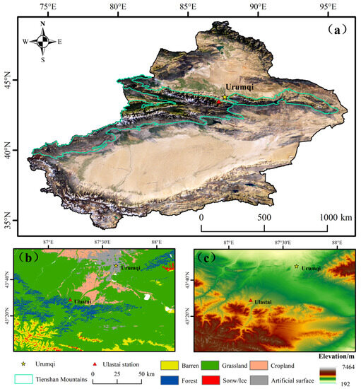
Figure 1.
(a) The specific locations of the Tien Shan and Ulastai station, (b) the land use types at the Ulastai station, and (c) the elevation map of the Ulastai station.
The footprint source area was analyzed using the Kljun footprint model [32] (Figure 2). In the range of 90% of flux footprint, portions of the footprint occupied by mountain grassland from April to September were 34%, 55%, 58%, 57%, 56%, and 55%, respectively. The radius of the 90% flux footprint fell within 1000 m, which indicated that the measured flux was majorly sourced from the mountain grassland surface and that the measured fluxes are representatives of this mountain grassland.
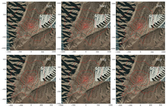
Figure 2.
The flux footprints of the test point from April to September of 2018. The outlines enclose 10–90% of the flux footprints.
2.2. Data Source
2.2.1. Measured Data Source
In 2016, the Urumqi Institute of Desert Meteorology, part of the China Meteorological Administration, established the Middle Tien Shan Grassland Land–Air Interaction Observation and Experimental Station in the Ulastai area of Baiyanggou, Urumqi. The station is equipped with an eddy covariance system, a radiation observation system, and a gradient detection system (Figure 3a). The data for this study were mainly obtained from three systems: (I) The eddy covariance system, which consists of a 3D sonic anemometer (CSAT3, Campbell Scientific, Logan, UT, USA) and an open-path infrared gas analyzer (Li7500A, Licor, Lincoln, NE, USA) (Figure 3c); we measure carbon flux using these two instruments. (II) The radiation observation system, which includes a net radiation sensor (CNR01, Kipp&Zonen, Logan, UT, USA, Figure 3b), a soil moisture sensor (CS616, USA), and a heat flow plate (HFP01, The Netherlands), was used to measure long-and short-wave radiation, soil moisture, and soil heat flux at different depths, respectively. (III) The gradient observation system includes a temperature and humidity sensor (HMP45C, Finland) for monitoring meteorological elements, such as soil temperatures at depths of 0 cm, 5 cm, 10 cm, and 20 cm, as well as air temperatures at heights of 2 m and 10 m. Figure 3d displays a 2D anemometer used to measure wind speed and wind direction. It is installed at a height of 2 m above the ground. It is worth noting that the underlying surface of the EC station is primarily grass, with a relatively dense coverage and good representativeness (Figure 3e).
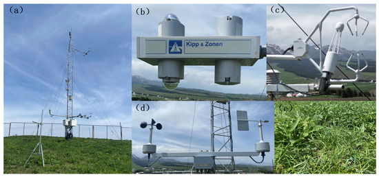
Figure 3.
(a) Ulastai station flux tower, (b) radiation observation system, (c) eddy covariance system; (d) 2D anemometer, and (e) photo of the underlying grassland, taken on 8 May 2023.
The measured data were output through a data collector (CR3000, Logan, UT, USA) at time intervals of 10 s, 1 min, 30 min, and 1 h. The radiation observation system and the gradient observation system were acquired at a frequency of 1 Hz, while the eddy covariance system was acquired at a frequency of 10 Hz. The time scale of this study is from April to September 2018, and all times used are local time.
2.2.2. Remote Sensing Data
The global carbon fluxes dataset (GCFD) is based on field carbon flux data, meteorological data, and remote sensing data. It utilizes convolutional neural network models (CNNs), artificial neural network models (ANNs), and random forest (RF) models to generate a global carbon flux dataset that includes net ecosystem exchange (NEE), gross primary productivity (GPP), and ecosystem respiration (Reco). The dataset has been validated and analyzed, revealing that NEE has lower accuracy compared to GPP and Reco in terms of temporal variability. However, the GCFD dataset fills in the gaps caused by the uneven distribution of global flux sites and the shortage of data in certain regions. The dataset has a spatial resolution of 1 km at three time steps per month from January 1999 to June 2020. The GCFD can be a useful reference for various meteorological and ecological analyses and modelling, especially when high resolution carbon flux maps are required [33] (Table 1). As per the GCFD data, the time scale is from April to September 2018, with a step of every 10 days, totaling 18 remote sensing images. We downloaded the GCFD dataset through the National Tibetan Plateau Data Center (https://dx.doi.org/10.11888/Terre.tpdc.300009, (accessed on 1 June 2023)).

Table 1.
Detailed information about the GCFD dataset.
2.3. Data Processing
2.3.1. Measured Data Processing
The EC system continuously observes CO2 flux, and the 30 min data observed via the EC system is processed using the EddyPro 7.1 software to ensure the accuracy of the observations. The original data underwent several processes to ensure accuracy. Initially, any outliers were removed. Subsequently, trend correction [34], the double rotation method [35], frequency response correction [36], sonic temperature correction [37], and Webb–Pearman–Leuning correction [38] were applied. Additionally, a turbulence stationarity test and an overall turbulence characteristic test were conducted to assess the quality of the data. Any data marked with flag 2 were excluded, and data with a frictional wind speed below the nighttime threshold were also eliminated.
Data imputation is particularly important due to various reasons, such as weather conditions, instrument failure, and quality control, which led to 22% of the CO2 flux data being missing from April to September of 2018. This issue causes inconvenience in the application of flux tower data. In the current investigation, an online data interpolation tool developed by the Biochemistry Department of the Max Planck Institute (https://www.bgc-jena.mpg.de/bgi/index.php/Services/REddyProcWeb, (accessed on 15 April 2023)) was used to interpolate the CO2 flux data. The method employs REddyProc in the R language package for data interpolation, which relies on meteorological data: total radiation, air temperature, and saturated water vapor pressure deficit (VPD) [39]. The data interpolation process consists of the following four steps: (I) Detection and rejection of (NEE) outliers. (II) Estimation of the night-time friction wind speed u* threshold. When the atmospheric turbulent motion is weak, the friction wind speed decreases, and the NEE measured via the eddy covariance system underestimates; therefore, the NEE data below the night-time friction wind speed u* threshold needs to be removed [40,41]. (III) Interpolation of NEE data by screening out data with time gaps and interpolating NEE using relevant meteorological and flux data [39]. (IV) The night-time data splitting method assumes that Reco is only related to temperature changes and that night-time vegetation only undergoes respiration. Therefore, the night-time NEE response curve to temperature can be used to infer the changes in vegetation Reco during the daytime. Finally, GPP can be calculated using Formula (1). The daytime data splitting method for NEE assumes that the relationship between daytime NEE and total radiation (Rg) and vapor pressure deficit (VPD) affects GPP, as well as the effect of temperature on Reco.
Due to the lack of instrumentation to observe saturated water vapor pressure, the empirical Tetens Equation (2) was used to indirectly estimate the saturated water vapor pressure from the air temperature using the relationship between the saturated water vapor pressure and the air temperature, as follows [42],
where T (°C) is the air temperature and e0(T) (ka) is the saturated water vapor pressure at temperature T.
2.3.2. Remote Sensing Data Processing
The GCFD data primarily utilize remote sensing and meteorological data as predictive factors. Remote sensing variables include the fraction of absorbed photosynthetically active radiation (FAPAR) and leaf area index (LAI), while meteorological variables include 2 m temperature (Ta), surface solar radiation downward (SW_IN), latent heat flux (LE), and sensible heat flux (H). FLUXNET 2015, FLUXNET-CH4, and Drought-2018 were used as site datasets, which include meteorological data and carbon flux variables. The remote sensing data, including FAPAR and LAI, were sourced from the Copernicus Global Land Service (CGLS) version 2 dataset, which has a 1 km resolution and covers the period from January 1999 to June 2020. The meteorological variable reanalysis data were sourced from the EAR5-Land dataset. With the above data, machine learning models are employed to predict global-scale NEE, GPP, and Reco.
Therefore, using GCFD data, the corresponding data for the Ulastai station is extracted and compared with the field-measured data for validation. The suitability of the GCFD data in the Ulastai region was evaluated using Pearson correlation coefficient (R), root mean square errors (RMSEs), and Bias indicators.
In the equation, represents the measured values and represents the GCFD data. and are the average values of the GCFD data and measured values, respectively; and and represent the measured values and GCFD data at each time step, respectively.
The specific methodological flow is shown in Figure 4.
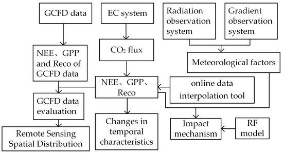
Figure 4.
Flowchart of the methodology in this study.
3. Results
3.1. Variation in CO2 Fluxes
3.1.1. Diurnal Variation in CO2 Fluxes
The results from the current investigation indicated the diurnal variations in CO2 fluxes during the growing season in the Middle Tien Shan grassland from April to September of 2018. NEE and GPP showed a “U”-shaped and inverted “U”-shaped trend, respectively, while Reco remained relatively constant with a mean value of 0.1 mg m−2 s−1 (Figure 5a). At 5:00, NEE showed a decreasing trend, while GPP showed an increasing trend. As the absorption rate of CO2 increased, the concentration of CO2 in the air gradually decreased, eventually causing NEE to reach a minimum value of −0.37 mg −2 s−1 at 11:00. After that, GPP gradually decreased as solar radiation weakened and photosynthesis in the grassland ecosystem slowed down, causing Reco to become the main source of CO2 fluxes at night and the concentration of CO2 in the air to rise. Overall, from 6:00 to 18:00, the grassland ecosystem acted as a carbon sink, while for the rest of the time, it acted as a carbon source.
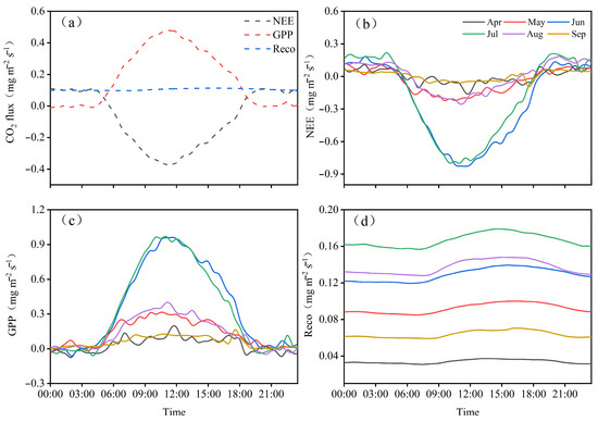
Figure 5.
(a) Diurnal variation in CO2 flux from April to September of 2018, (b) diurnal variation in net ecosystem exchange (NEE) from April to September of 2018, (c) diurnal variation in gross primary productivity (GPP) from April to September of 2018, and (d) diurnal variation in ecosystem respiration (Reco) from April to September of 2018.
NEE, GPP, and Reco varied in each month of the growing season (Figure 5b–d). As solar height and solar radiation are stronger from June to August than in other months, the changes in NEE and GPP were most pronounced in June and July, while the changes in Reco were most pronounced in July and August. Thus, carbon sources and sinks in grassland ecosystems showed greater changes in June and July than in other months. The daily average values of NEE ranged from −0.24 to 0.004 mg m−2 s−1, GPP ranged from 0.03 to 0.37 mg m−2 s−1, and Reco ranged from 0.03 to 0.17 mg m−2 s−1 from April to September of 2018.
3.1.2. Daily and Monthly Variations of CO2 Fluxes
Figure 5 shows the daily and monthly variations in CO2 fluxes during the growing season in the Middle Tien Shan grassland from April to September of 2018. NEE, GPP, and Reco all exhibit significant seasonal variation, with NEE and GPP showing opposite trends (Figure 6a). The maximum CO2 uptake occurred on 17 June, at −9.73 g C m−2 d−1, and NEE showed CO2 uptake from 15 May to 6 August, during which time the grassland ecosystem acted as a carbon sink. GPP varied from −2.48 to 13.18 g C −2 d−1, with a mean value of 4.26 g C m−2 d−1. Reco variation was relatively stable, ranging from 0.12 to 5.63 g C m−2 d−1, with a mean value of 2.46 g C m−2 d−1, which was significantly lower than GPP. In addition, Reco showed a slow upward trend in June and July, due to increased solar radiation and vigorous grass growth compared to other months, resulting in enhanced ecosystem respiration.
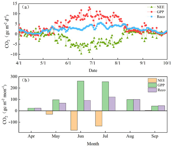
Figure 6.
(a) Daily variation in net ecosystem exchange (NEE), gross primary productivity (GPP), and ecosystem respiration (Reco) in grassland ecosystems from April to September of 2018, (b) monthly variations of net ecosystem exchange (NEE), gross primary productivity (GPP) and ecosystem respiration (Reco) in grassland ecosystems from April to September of 2018.
The monthly variation in CO2 fluxes in grassland ecosystems is shown in Figure 6b. The maximum monthly accumulation of NEE and GPP occurred in June, with −170.01 g C m−2 mon−1 and 261.27 g C m−2 mon−1, respectively, and the maximum monthly accumulation of Reco occurred in July, with 121.80 g C m−2 mon−1. During June and July, grassland ecosystems were in their peak growing season, showing CO2 flux uptake, which was manifested as carbon sinks, while the rest of the months acted as carbon sources. April and September, the beginning and end of the growing season, respectively, were the months when photosynthesis and respiration were weaker in grass compared to other months. Therefore, the uptake or release of CO2 fluxes was lowest throughout the growing season. The overall accumulation of NEE, GPP, and Reco during the growing season was −329.49 g C m−2, 779.04 g C m−2, and 449.55 g C m−2, respectively.
3.2. Impact of Meteorological Factors on CO2 Fluxes
3.2.1. Seasonal Variation in Meteorological Factors
Figure 6 illustrates the changes in the growing season characteristics of the main meteorological factors in the grassland ecosystem from April to September of 2018. Wind speed (WS) changed relatively smoothly, with a range of 0.01–4.48 m/s and an average of 2.42 m/s. The largest change occurred in April (Figure 7a). Relative humidity (RH) generally exhibited a slowly fluctuating downward trend, with smaller fluctuations from June to August. Meanwhile, the water vapor mass in the saturated air at the same temperature and pressure remained constant or increased, resulting in a slowly fluctuating downward trend in RH (Figure 7b). Photosynthetic active radiation (PAR) exhibited relatively minor variations in June, July, and August compared to other months (Figure 7c). The saturation water vapor pressure difference (VPD) increased with rising temperatures in June, July, and August (Figure 7d). In June, July, and August, both air temperature (Ta) and soil temperature (Ts) were higher, while they were lowest in April. The air temperature (Ta) overall showed a normal distribution, with mean values of 10.85 °C and 10.86 °C at 2 m and 10 m, respectively. The soil temperature at 0 cm varied more, while the soil temperature at 20 cm varied less, and the soil temperature was similar in all strata (Figure 7e,f). Soil moisture content (SWC) varied significantly among the strata, with the highest value at 5 cm, the lowest at 20 cm, and the second-highest at 10 cm, with mean values of 0.22 m3/m3, 0.18 m3/m3, and 0.12 m3/m3, respectively (Figure 7g). Soil heat flux (SHF) showed a slowly decreasing trend overall, with significant changes in April and May, and then leveled off in the remaining months (Figure 7h).
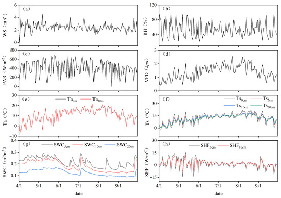
Figure 7.
Seasonal variation in meteorological factors in grassland ecosystems from Apr to Sept of 2018. (a) Seasonal variation in wind speed (WS); (b) seasonal variation in relative humidity (RH); (c) seasonal variation in photosynthetic active radiation (PAR); (d) seasonal variation in vapor pressure difference (VPD); (e) seasonal variation in air temperature (Ta); (f) seasonal variation in soil temperature (Ts); (g) seasonal variation in soil moisture content (SWC); and (h) seasonal variation in Soil heat flux (SHF).
3.2.2. Contribution of Meteorological Factors to CO2 Fluxes
The machine learning algorithm, random forest (RF), has the advantage of being able to handle large amounts of mixed data with high noise immunity and assess the importance of each variable factor [43]. Therefore, the contribution of meteorological factors to CO2 fluxes at half-hourly and daily scales was calculated using the RF model.
As shown in Figure 8, at the half-hourly scale, the 0 cm soil temperature had the greatest contribution to NEE and GPP, while the 20 cm soil temperature had the largest contribution to Reco. It is noteworthy that for the studied seasonal variations and control factors of water and CO2 flux in alpine meadows in Lijiang, southwestern China, using eddy covariance technology on half-hourly and daily scales, photosynthetically active radiation (PAR) and air temperature are the primary meteorological factors determining net ecosystem production (NEP) [44]. At the daily scale, the 20 cm soil moisture contributed the most to NEE and GPP, followed by the 10 cm and 20 cm soil temperature, and the 5 cm soil temperature contributed the most to Reco. This indicates that soil temperature is a prerequisite for the variation in CO2 fluxes in the Middle Tien Shan grassland ecosystem because temperature affects the enzyme activity of plant physiological processes, which in turn affects photosynthesis in the ecosystem. It also suggests that the meteorological factor of soil temperature has the most significant influence on CO2 fluxes, both at the half-hourly and daily scales.
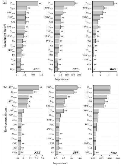
Figure 8.
Ranking of the contribution of meteorological factors affecting CO2 fluxes. (a) On a half-hourly scale; and (b) on a daily scale. ** represents passing the 99% significance test; * represents passing the 95% significance test.
3.3. Response of CO2 Fluxes to Temperature
3.3.1. Relationship between CO2 Fluxes and Temperature
To further characterize the effect of soil temperature on CO2 fluxes, we fitted the function curves of soil temperature and CO2 fluxes for each stratum (Figure 9). The study showed that soil temperature and CO2 fluxes at different depths exhibited a univariate linear regression, and the correlation between soil temperature and CO2 fluxes improved with the increasing soil temperature. Soil temperature and NEE at different depths exhibited a negative correlation, meaning that NEE decreased as the soil temperature increased. The correlations between Ts0cm, Ts5cm, Ts10cm, and Ts20cm with NEE are 0.04, 0.09, 0.10, and 0.11, respectively (Figure 9a–d). The correlation between soil temperature and GPP at different depths was positive, indicating that the respiration of the grassland ecosystem increased more than photosynthesis with the increase in soil temperature, leading to increased GPP. The correlations between Ts0cm, Ts5cm, Ts10cm, and Ts20cm with GPP are 0.16, 0.25, 0.26, and 0.27, respectively (Figure 9e–h). The relationship between soil temperature at different depths and NEE and GPP was tested for significance, effectively demonstrating that soil temperature is an important indicator influencing carbon flux in the Middle Tien Shan grassland ecosystem.
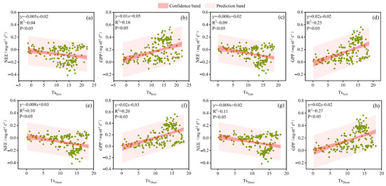
Figure 9.
Relationship between CO2 fluxes and soil temperature at different depths. (a) The relationship between 0 cm soil temperature and NEE, (b) the relationship between 0 cm soil temperature and GPP, (c) the relationship between 5 cm soil temperature and NEE, (d) the relationship between 5 cm soil temperature and GPP, (e) the relationship between 10 cm soil temperature and NEE, (f) the relationship between 10 cm soil temperature and GPP, (g) the relationship between 20 cm soil temperature and NEE, and (h) the relationship between 20 cm soil temperature and GPP.
To further investigate the effect of temperature on carbon fluxes in grassland ecosystems, a curve was fitted as a function of temperature and CO2 fluxes using different temperature gradients (Figure 10). From the figure, it can be observed that, similarly to the relationship between soil temperature and CO2 fluxes, the temperature of different gradients showed a univariate linear regression with a negative correlation between NEE and temperature, and an exponential distribution with a positive correlation between GPP and temperature. The correlation between air temperature and CO2 fluxes was significantly higher than that of soil temperature, indicating that air temperature is also an important factor in regulating CO2 fluxes in grassland ecosystems. However, the contribution of air temperature to CO2 fluxes was significantly lower than that of soil temperature (Figure 8).
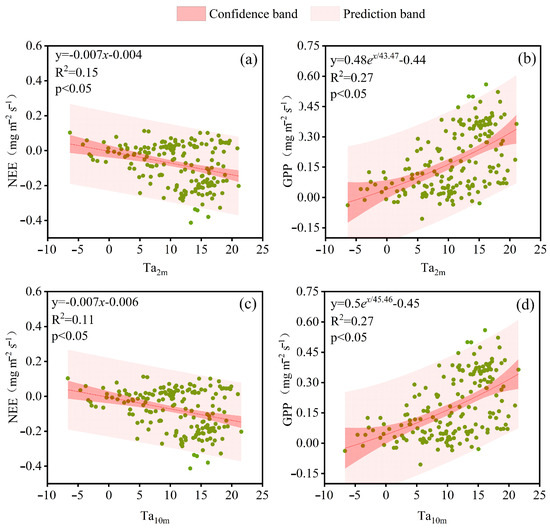
Figure 10.
Relationship between CO2 fluxes and air temperature with different gradients. (a) The relationship between 2 m air temperature and NEE, (b) the relationship between 2 m air temperature and GPP, (c) the relationship between 10 m air temperature and NEE, and (d) the relationship between 10 m air temperature and GPP.
3.3.2. Critical Values of Temperature Effects on CO2 Fluxes
The soil and air temperatures were divided into eight and six intervals, respectively, to investigate CO2 fluxes in different temperature ranges (Figure 11). The study showed that as the temperature increased, NEE tended to decrease and then increase, with a “turning point” at 25 °C (Figure 11a). When the soil temperature reaches 25 °C, it provides an optimal temperature for vegetation growth, and the stomata of vegetation roots open to efficiently absorb photosynthetic radiation and increase the photosynthetic absorption rate [16]. At this point, photosynthesis is greater than respiration in grassland ecosystems, leading to a relatively low concentration of CO2 in the air and causing the grassland to generally act as a carbon sink. When the soil temperature drops to below 15 °C, vegetation is vulnerable to cold stress, and prolonged low temperatures are detrimental to crop growth and development, leading to reduced photosynthesis in the grassland ecosystem. This, in turn, weakens photosynthesis, causing CO2 fluxes in the air to begin rebounding (Figure 11b). The trend of GPP is opposite to that of NEE, and the critical soil temperature for GPP is 25 °C (Figure 11c). The critical soil temperature for the effect on Reco is 10 °C. Reco begins to increase when the soil temperature exceeds 10 °C and reaches its maximum value when the soil temperature is above 40 °C (Figure 11e).
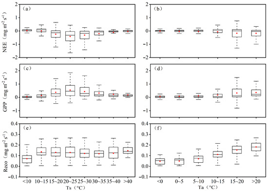
Figure 11.
Critical values of the effect of soil temperature and air temperature on CO2 flux. (a,c,e) Critical values of the effect of soil temperature on CO2 flux, and (b,d,f) critical values of the effect of air temperature on CO2 flux.
NEE decreases gradually with increasing air temperature, and changes more smoothly when the air temperature is below 15 °C. However, it decreases more rapidly when the air temperature exceeds 15 °C (Figure 11b). Conversely, the trend of GPP is opposite to that of NEE, with GPP showing an increasing trend when the temperature exceeds 15 °C (Figure 11d). Nonetheless, Reco increases with temperature and does not demonstrate a critical value due to its unique geographical location with relatively low temperatures.
3.4. The Trend of Carbon Flux at the Regional Scale
3.4.1. Assessment of the Applicability of GCFD Data
Figure 12 shows a comparison between the field-measured values of carbon flux and the GCFD data during the 2018 growing season in the Tian Shan grassland. The field-measured values of NEE, GPP, and Reco show a high correlation with the GCFD data. Compared to GPP and Reco, the correlation between the field-measured values of NEE and the GCFD data is relatively low at 0.59, while the correlation between the field-measured values of GPP and Reco and the GCFD data is 0.81 and 0.73, respectively. The RMSEs are 5.21, 4.99, and 2.20, and the Bias values are 0.41, 0.19, and 0.94, respectively (Figure 12a–c). The variations in the field-measured values and the GCFD data are generally in phase. The field-measured values of NEE and the GCFD data show a reversed “U”-shape trend, reaching their minimum values in June and July. However, the field-measured values have a larger magnitude of variation compared to the GCFD data. The field-measured values of GPP and Reco exhibit the same trend as the GCFD data. Starting from April, both the field-measured values and the GCFD data show an increasing trend, reaching their peak values in July, followed by a decreasing trend. However, the field-measured values have a larger magnitude of variation compared to the GCFD data. The trend of Reco in the field-measured data is similar to that of GPP, with both reaching their maximum values in July. However, the GCFD data overall tend to overestimate compared to the field-measured values (Figure 12d–f).
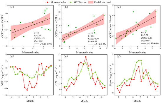
Figure 12.
Comparison and validation of the GCFD data and the measured value at the Ulastai Station from April to September of 2018. (a–c) The correlation and error between GCFD data and measured value of CO2 flux data, and (d–f) comparison of the trend changes between GCFD data and measured value of CO2 flux data.
3.4.2. Remote Sensing Distribution of the GCFD Dataset
Figure 13 shows a remote sensing distribution map of the average carbon flux during the growing season in the Tien Shan region of Xinjiang in 2018. The minimum overall change in NEE occurs in the Ili River Valley, which is −5.91 mg m−2 s−1. This is because the Ili River Valley has a significantly warmer and moister climate compared to other regions from April to September, leading to vigorous vegetation growth. During this time, photosynthesis exceeds respiration, resulting in a lower CO2 flux in the air and the occurrence of a carbon sink phenomenon. In contrast, in the eastern and western regions of Tien Shan, where there are more high mountains and glaciers, the sparse vegetation leads to a less pronounced carbon sink phenomenon. Ulastai station shows a more significant carbon sink phenomenon, with an average NEE value of −1.48 mg m−2 s−1 during the growing season. This is due to the thriving grassland ecosystem in the Ulastai station from April to September. The overall changes in GPP and Reco in the Tien Shan region exhibit an opposite trend to NEE, with the maximum values occurring in the Ili River Valley at 11.58 mg m−2 s−1 and 12.35 mg m−2 s−1, respectively. The average values in the Ulas Plateau during the growing season are 4.44 mg m−2 s−1 for GPP and 3.22 mg m−2 s−1 for Reco.
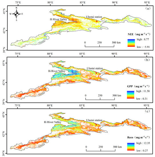
Figure 13.
Average seasonal distribution of carbon flux in the Tien Shan region from April to September of 2018. (a) NEE, (b) GPP, and (c) Reco.
4. Discussion
4.1. Variations inCO2 Fluxes
The NEE of the Middle Tien Shan grassland ecosystem showed an overall “U” curve change from April to September 2018. The ecosystem acted as a net carbon sink during the day and a net carbon source during the night. At 5:00, NEE showed a decreasing trend, while GPP showed an increasing trend due to the increase in solar height and radiation, leading to greater levels of photosynthesis than respiration in the grassland ecosystems [45]. This conclusion is consistent with the findings of previous research conducted by Du et al. in wetlands [18]. In terms of daily variation, NEE and GPP showed opposite trends, with the maximum CO2 uptake occurring on June 17 at −9.73 g C m−2 d−1. Similar findings were reported in a study of a rice ecosystem in the Khorqin grassland; the difference is that Bao et al. found that in the rice ecosystem, the maximum CO2 uptake occurs on August 15th, with a value of −17.89 g C−2 d−1 [19]. In terms of monthly variation, the overall cumulative CO2 flux in the growing season of the Middle Tien Shan grassland ecosystem from April to September was −329.49 g C m−2, 779.04 g C m−2, and 449.55 g C m−2, respectively. Compared to the reported CO2 flux of −183.45 g C m−2 in the growing season of the desert ecosystem in the Gurbantunggut Desert by Gulnur et al. [46], this indicates that the carbon sequestration capacity of grassland ecosystems in the arid region of northwest China is higher than that of desert ecosystems.
Compared to other terrestrial ecosystems (Table 2), the Middle Tien Shan grassland ecosystem has a weaker carbon sink capacity than the forest [47] and meadow-rice ecosystems [19], but a stronger capacity than marsh and Siberian bog ecosystem [18,48]. The hydrothermal conditions play a crucial role in affecting the strength of carbon sequestration [49]. The sandy grassland of Horqin has a substratum dominated by fine sand and clay-powder grains that strongly absorb solar radiation, resulting in an increased potential evapotranspiration, and combined with less precipitation; this leads to a stronger carbon sequestration capacity of the Middle Tien Shan grassland ecosystem compared to the sandy grassland ecosystem of Horqin [50]. In comparison to the grassland ecosystem of the Yunnan–Guizhou plateau [12], the carbon sequestration capacity of the Middle Tien Shan grassland ecosystem is weaker. The Yunnan–Guizhou plateau belongs to the subtropical climate zone with abundant water and heat conditions, while the Middle Tien Shan grasslands belong to the typical temperate continental climate with less precipitation and a dry climate. This weaker capacity of carbon sequestration in the Middle Tien Shan grassland ecosystem is due to the lack of water and heat conditions.
Table 2.
Comparison of CO2 fluxes in different types of terrestrial ecosystems (values marked with * indicate that the study time scale is one year).
4.2. The Relationship between CO2 Fluxes and Meteorological Factors and Their Response to Temperature
The RF model was used to calculate the correlation between CO2 fluxes and meteorological factors in the Middle Tien Shan grassland ecosystem, and it was found that soil temperature was the main meteorological factor affecting CO2 fluxes. As the soil temperature increased, the NEE of the Middle Tien Shan grassland ecosystem decreased, while GPP and Reco increased. This study is consistent with the previous conclusion that GPP and Reco increase significantly with global warming [51]. The carbon sink during the growing season occurs in June and July, which is consistent with favorable water and thermal conditions, despite the highest temperature occurring in August. This result may be attributed to the extreme drought climate in August, indicating that water and thermal conditions are important factors limiting photosynthesis in arid vegetation [52]. In August, grassland ecosystems were susceptible to high-temperature stress due to enhanced solar height and solar radiation, which, together with low precipitation, accelerated the shortening of the grassland phenological cycle, leading to increased potential evapotranspiration and respiration in the grasslands. Enhanced evapotranspiration could lead to water stress in plants [53], resulting in weaker CO2 flux uptake and release in grassland ecosystems, as well as weaker GPP and Reco. Previous studies have shown that drought or high temperatures cause the CO2 balance of arid and semi-arid ecosystems to shift from carbon sink to carbon source [54,55,56,57].
The grassland ecosystem had the strongest carbon sequestration capacity when the soil temperature is 25 °C. Above this temperature, the grassland ecosystem is prone to heat stress, while below this temperature, it is susceptible to cold stress. The current investigation confirms this conclusion, finding that when soil temperature rises above 35 °C, extreme drought conditions are highly likely to occur. Drought and high temperatures lead to dehydration of grass cells, and the lack of water and heat conditions adversely affect the photosynthesis of grassland [58]. When the soil temperature exceeds 10 °C, the Reco of grassland ecosystems begins to increase. As the soil temperature surpasses 40 °C, Reco reaches its maximum value. Air temperature also had a strong correlation with carbon fluxes in the grassland ecosystems, which was consistent with previous studies [59,60,61]. In our research, we have discovered that the temperature threshold for the occurrence of carbon sinks in grassland ecosystems is 15 °C. This further demonstrates that vegetation requires the most suitable temperature for growth through photosynthesis [62].
4.3. Remote Sensing Carbon Flux
Through a comparison and analysis of field measurement data from the Ulastai Station in the Middle Tien Shan grassland ecosystem, it was found that the GCFD data are applicable to the Ulastai region. The correlation coefficients between GCFD data and the measured values of NEE, GPP, and Reco are 0.59, 0.81, and 0.73, respectively. The accuracy of GPP and Reco in the GCFD dataset was higher than NEE, which is consistent with the conclusions reached by Shangguan et al. [33]. The RMSE values for the GCFD data compared to the measured values of NEE, GPP, and Reco are 5.21, 4.99, and 2.20, respectively, the Bias values are 0.41, 0.19, and 0.94. The reason for this error may be due to the fact that the training samples were selected from 280 global sites, mainly distributed in Europe and North America. Additionally, there may be regions with a lack of observational data, resulting in inaccurate simulated accuracy and errors between the site measurements and the GCFD dataset. Furthermore, there is an imbalance in the temporal and spatial resolutions of the remote sensing data, meteorological data, and carbon flux data used in the GCFD dataset. To unify the spatiotemporal resolution, the time resolution for these three types of data is set to 10 days per step, and the spatial resolution is set to 1 km. This process may introduce deviations in the dataset results [63,64].
Figure 12 presents the remote sensing spatial distribution of carbon flux in the Tien Shan region of Xinjiang. The Ulastai area shows a significant carbon sink from April to September 2018, with the highest carbon sink value occurring in the Ili River Valley, which is consistent with previous studies [65]. Therefore, through the verification analysis of field measurement data from the eddy correlation system and GCFD data, it was shown that the errors in the GCFD dataset resulting from the uneven distribution of training sample sites and unified spatiotemporal resolution are not significant for evaluating global carbon cycling. The example of Ulastai Station provides a scientific basis for the application of GCFD data in other regions. It also verifies the feasibility of using a machine learning fusion algorithm to construct a carbon flux dataset and provide data support for areas with sparse measurements.
5. Conclusions
The focus of this study was on the characteristics of carbon dioxide fluxes during the growing season and their response to temperature in the grassland ecosystems of the Middle Tien Shan Mountains in Xinjiang. The grassland ecosystems acted as carbon sinks during the daytime from 6:00 to 18:00 and as carbon sources during the rest of the day. Due to the increase in solar altitude and solar radiation, the carbon dioxide flux of the grassland ecosystem changed most in June, July and August, with June and July showing significant carbon sinks. The soil temperature and air temperature at different depths were negatively correlated with NEE and positively correlated with GPP and Reco. The carbon sequestration capacity of the grassland ecosystems was strongest when the soil temperature was 25 °C.
The GCFD data were compared and analyzed with the data from the Ulastai station. They show a high correlation and small errors compared to the measured value. This dataset is highly applicable in the Ulastai region and has consistent remote sensing spatial distribution. The GCFD dataset can clearly demonstrate the characteristic changes in carbon flux in the Tien Shan region, providing possibilities for the future application of GCFD data in other areas.
This study only used the 2018 growing season eddy covariance data to explore the carbon flux balance. The carbon flux variation characteristics of grassland ecosystems during the non-growing season is worth further investigations. Additionally, this study only utilized site-specific data to reveal the influencing mechanisms of carbon flux in grassland ecosystems, which implies the need for further exploration of the influencing mechanisms of carbon flux in remote sensing space.
Author Contributions
Conceptualization, K.Z. and A.M.; methodology, K.Z. and Y.L.; software, Y.W.; validation, C.W. and M.S.; formal analysis, F.Y., C.Z. and W.H.; data curation, J.G. and A.A.; resources, A.M.; writing—original draft preparation, K.Z.; writing—review and editing, K.Z., A.M. and Y.L.; visualization, K.Z. All authors have read and agreed to the published version of the manuscript.
Funding
This research was funded by the Special Project for the Construction of Innovation Environment in the Autonomous Region (PT2203), the Special Funds for Basic Scientific Research Business Expenses of Central-level Public Welfare Scientific Research Institutes (IDM2021005), the Scientific and Technological Innovation Team (Tien Shan Innovation Team) project (grant No. 2022TSYCTD0007), the National Natural Science Foundation of China (grant No. 41875023), the S&T Development Fund of IDM (KJF202302), the Special Funds for Basic Scientific Research Business Expenses of Central-level Public Welfare Scientific Research Institutes (IDM2021001), and the Graduate Education Innovation Program of the Autonomous Region (XJ2023G032).
Data Availability Statement
The data used in this paper can be obtained from A.M. (ali@idm.cn) upon request.
Acknowledgments
The carbon flux data of the eddy covariance system were provided by the Urumqi Desert Meteorological Research Institute of the China Meteorological Administration. The GCFD dataset was provided by the National Tibetan Plateau Scientific Data Center.
Conflicts of Interest
All authors declare no conflict of interest.
References
- Pachauri, R.K.; Reisinger, A. IPCC fourth assessment report. IPCC Geneva 2007, 2007, 044023. [Google Scholar]
- Liu, H.Z.; Tu, G.; Fu, C.B.; Shi, L.Q. Three-year Variations of Water, Energy and CO2 Fluxes of Cropland and Degraded Grassland Surfaces in a Semi-arid Area of Northeastern China. Adv. Atmos. Sci. 2008, 25, 1009–1020. [Google Scholar] [CrossRef]
- Tans, P.P.; Fung, I.Y.; Takahashi, T. Observational contrains on the global atmospheric CO2 budget. Science 1990, 247, 1431–1438. [Google Scholar] [CrossRef] [PubMed]
- Gao, G.Z.; Wang, M.L.; Li, D.H.; Li, N.N.; Wang, J.Y.; Niu, H.H.; Meng, M.; Liu, Y.; Zhang, G.H.; Jie, D.M. Phytolith evidence for changes in the vegetation diversity and cover of a grassland ecosystem in Northeast China since the mid-Holocene. Catena 2023, 226, 107061. [Google Scholar] [CrossRef]
- Bai YF, C.S. Carbon sequestration of Chinese grassland ecosystems: Stock, rate, and potential. Chin. J. Plant Ecol. 2018, 42, 261–264. [Google Scholar]
- Wang, Y.Y.; Xiao, J.F.; Ma, Y.M.; Luo, Y.Q.; Hu, Z.Y.; Li, F.; Li, Y.N.; Gu, L.L.; Li, Z.G.; Yuan, L. Carbon fluxes and environmental controls across different alpine grassland types on the Tibetan Plateau. Agric. For. Meteorol. 2021, 311, 108694. [Google Scholar] [CrossRef]
- Ma, Z.L.; Bork, E.W.; Attaeian, B.; Cahill, J.F.; Chang, S.X. Altered precipitation rather than warming and defoliation regulate short-term soil carbon and nitrogen fluxes in a northern temperate grassland. Agric. For. Meteorol. 2022, 327, 109217. [Google Scholar] [CrossRef]
- Shi, L.A.; Lin, Z.R.; Tang, S.M.; Peng, C.J.; Yao, Z.Y.; Xiao, Q.; Zhou, H.K.; Liu, K.S.; Shao, X.Q. Interactive effects of warming and managements on carbon fluxes in grasslands: A global meta-analysis. Agric. Ecosyst. Environ. 2022, 340, 108178. [Google Scholar] [CrossRef]
- Argenti, G.; Chiesi, M.; Fibbi, L.; Maselli, F. Use of remote sensing and bio-geochemical models to estimate the net carbon fluxes of managed mountain grasslands. Ecol. Model. 2022, 474, 110152. [Google Scholar] [CrossRef]
- Bai, Y.F.; Han, X.G.; Wu, J.G.; Chen, Z.Z.; Li, L.H. Ecosystem stability and compensatory effects in the Inner Mongolia grassland. Nature 2004, 431, 181–184. [Google Scholar] [CrossRef]
- Jia, X.; Zha, T.S.; Gong, J.N.; Zhang, Y.Q.; Wu, B.; Qin, S.G.; Peltola, H. Multi-scale dynamics and environmental controls on net ecosystem CO2 exchange over a temperate semiarid shrubland. Agric. For. Meteorol. 2018, 259, 250–259. [Google Scholar] [CrossRef]
- Sun, S.-S.; Wu, Z.-P.; Xiao, Q.-T.; Yu, F.; Gu, S.-H.; Fang, D.; LI, L.; Zhao, X.-B. Factors influencing CO2 fluxes of a grassland ecosystem on the Yunnan-Guizhou Plateau, China. Acta Prataculturae Sin. 2020, 29, 184. [Google Scholar]
- Shen, H.; Zhu, Y.; Zhao, X.; Geng, X.; Gao, S.; Fang, J. Analysis of current grassland resources in China. Chin. Sci. Bull. 2016, 61, 139–154. [Google Scholar]
- Chen, C.B.; Peng, J.; Li, G.Y. Evaluating ecosystem health in the grasslands of Xinjiang. Arid. Zone Res. 2022, 39, 270–281. [Google Scholar] [CrossRef]
- Fang, X.; Guo, X.L.; Zhang, C.; Shao, H.; Zhu, S.H.; Li, Z.Q.; Feng, X.W.; He, B. Contributions of climate change to the terrestrial carbon stock of the arid region of China: A multi-dataset analysis. Sci. Total Environ. 2019, 668, 631–644. [Google Scholar] [CrossRef]
- Guo, W.Z.; Jing, C.Q.; Deng, X.J.; Chen, C.; Zhao, W.K.; Hou, Z.X.; Wang, G.X. Variations in carbon flux and factors influencing it on the northern slopes of the TienShan Mountains. Acta Prataculturae Sin. 2022, 31, 1–12. [Google Scholar] [CrossRef]
- Yang, F.; Huang, J.P.; He, Q.; Zheng, X.Q.; Zhou, C.L.; Pan, H.L.; Huo, W.; Yu, H.P.; Liu, X.Y.; Meng, L.; et al. Impact of differences in soil temperature on the desert carbon sink. Geoderma 2020, 379, 114636. [Google Scholar] [CrossRef]
- Du, Q.; Liu, H.Z.; Liu, Y.; Xu, L.J.; Sun, J.H. Water and carbon dioxide fluxes over a “floating blanket” wetland in southwest of China with eddy covariance method. Agric. For. Meteorol. 2021, 311, 108689. [Google Scholar] [CrossRef]
- Bao, Y.Z.; Liu, T.X.; Duan, L.M.; Tong, X.; Zhang, Y.Q.; Wang, G.Q.; Singh, V.P. Variations and controlling factors of carbon dioxide and methane fluxes in a meadow-rice ecosystem in a semi-arid region. Catena 2022, 215, 106317. [Google Scholar] [CrossRef]
- Li, R.; Zhang, M.; Chen, L.; Kou, X.; Skorokhod, A. CMAQ simulation of atmospheric CO2 concentration in East Asia: Comparison with GOSAT observations and ground measurements. Atmos. Environ. 2017, 160, 176–185. [Google Scholar] [CrossRef]
- Wang, J.; Lu, S.; Wang, W.; Tang, L.; Ma, S.; Wang, Y. Estimating vegetation productivity of urban regions using sun-induced chlorophyll fluorescence data derived from the OCO-2 satellite. Phys. Chem. Earth Parts A/B/C 2019, 114, 102783. [Google Scholar] [CrossRef]
- Kunchala, R.K.; Patra, P.K.; Kumar, K.N.; Chandra, N.; Attada, R.; Karumuri, R.K. Spatio-temporal variability of XCO2 over Indian region inferred from Orbiting Carbon Observatory (OCO-2) satellite and Chemistry Transport Model. Atmos. Res. 2022, 269, 106044. [Google Scholar] [CrossRef]
- Zhang, Z.; Guanter, L.; Porcar-Castell, A.; Rossini, M.; Pacheco-Labrador, J.; Zhang, Y. Global modeling diurnal gross primary production from OCO-3 solar-induced chlorophyll fluorescence. Remote Sens. Environ. 2023, 285, 113383. [Google Scholar] [CrossRef]
- Yao, F.; Qin, P.; Zhang, J.; Lin, E.; Boken, V. Uncertainties in assessing the effect of climate change on agriculture using model simulation and uncertainty processing methods. Chin. Sci. Bull. 2011, 56, 729–737. [Google Scholar] [CrossRef]
- Wilkin, J.; Levin, J.; Moore, A.; Arango, H.; López, A.; Hunter, E. A data-assimilative model reanalysis of the US Mid Atlantic Bight and Gulf of Maine: Configuration and comparison to observations and global ocean models. Prog. Oceanogr. 2022, 209, 102919. [Google Scholar] [CrossRef]
- Zhang, F.; Lu, X.; Huang, Q.; Jiang, F. Impact of different ERA reanalysis data on GPP simulation. Ecol. Inform. 2022, 68, 101520. [Google Scholar] [CrossRef]
- Yang, P.; Wang, N.A.; Zhao, L.Q.; Zhang, D.Z.; Zhao, H.; Niu, Z.M.; Fan, G.Q. Variation characteristics and influencing mechanism of CO2 flux from lakes in the Badain Jaran Desert: A case study of Yindeer Lake. Ecol. Indic. 2021, 127, 107731. [Google Scholar] [CrossRef]
- Zhou, Y.Y.; Sachs, T.; Li, Z.; Pang, Y.W.; Xu, J.F.; Kalhori, A.; Wille, C.; Peng, X.X.; Fu, X.H.; Wu, Y.F.; et al. Long-term effects of rewetting and drought on GPP in a temperate peatland based on satellite remote sensing data. Sci. Total Environ. 2023, 882, 163395. [Google Scholar] [CrossRef]
- Chen, Y.; Li, Z.; Fang, G.; Deng, H. Impact of climate change on water resources in the Tianshan Mountians. Cent. Asia. Acta Geogr. Sin. 2017, 72, 18–26. [Google Scholar]
- Xiao, W.Q.; Ali, M.; Liu, Y.Q.; Wang, Y.; Gao, J.; Hajigul, S.; Gurinisahan, M. The rule of grassland surface radiation budget in the middle of TienShan Mountains. Acta Ecol. Sin. 2022, 42, 4550–4560. [Google Scholar]
- Sang, W. Plant diversity patterns and their relationships with soil and climatic factors along an altitudinal gradient in the middle Tianshan Mountain area, Xinjiang, China. Ecol. Res. 2009, 24, 303–314. [Google Scholar] [CrossRef]
- Kljun, N.; Calanca, P.; Rotach, M.W.; Schmid, H.P. A simple two-dimensional parameterisation for Flux Footprint Prediction (FFP). Geosci. Model Dev. 2015, 8, 3695–3713. [Google Scholar] [CrossRef]
- Shangguan, W.; Xiong, Z.; Nourani, V.; Li, Q.; Lu, X.; Li, L.; Huang, F.; Zhang, Y.; Sun, W.; Dai, Y. A 1 km Global Carbon Flux Dataset Using In Situ Measurements and Deep Learning. Forests 2023, 14, 913. [Google Scholar] [CrossRef]
- Rannik, U.; Vesala, T. Autoregressive filtering versus linear detrending in estimation of fluxes by the eddy covariance method. Bound. -Layer Meteorol. 1999, 91, 259–280. [Google Scholar] [CrossRef]
- Kaimal, J.C.; Finnigan, J.J. Atmospheric boundary Layer Flows: Their Structure and Measurement; Oxford University Press: Oxford, UK, 1994. [Google Scholar]
- Moore, C.J. Frequency-response corrections for eddy-correlation systems. Bound.-Layer Meteorol. 1986, 37, 17–35. [Google Scholar] [CrossRef]
- Schotanus, P.; Nieuwstadt, F.T.M.; Debruin, H.A.R. Temperature-measurement with a sonic anemometer and its application to heat and moisture fluxes. Bound.-Layer Meteorol. 1983, 26, 81–93. [Google Scholar] [CrossRef]
- Webb, E.K.; Pearman, G.I.; Leuning, R. Correction of flux measurements for density effects due to heat and water-vapor transfer. Q. J. R. Meteorol. Soc. 1980, 106, 85–100. [Google Scholar] [CrossRef]
- Reichstein, M.; Falge, E.; Baldocchi, D.; Papale, D.; Aubinet, M.; Berbigier, P.; Bernhofer, C.; Buchmann, N.; Gilmanov, T.; Granier, A.; et al. On the separation of net ecosystem exchange into assimilation and ecosystem respiration: Review and improved algorithm. Glob. Chang. Biol. 2005, 11, 1424–1439. [Google Scholar] [CrossRef]
- Papale, D.; Reichstein, M.; Aubinet, M.; Canfora, E.; Bernhofer, C.; Kutsch, W.; Longdoz, B.; Rambal, S.; Valentini, R.; Vesala, T.; et al. Towards a standardized processing of Net Ecosystem Exchange measured with eddy covariance technique: Algorithms and uncertainty estimation. Biogeosciences 2006, 3, 571–583. [Google Scholar] [CrossRef]
- Desai, A.R.; Richardson, A.D.; Moffat, A.M.; Kattge, J.; Hollinger, D.Y.; Barr, A.; Falge, E.; Noormets, A.; Papale, D.; Reichstein, M.; et al. Cross-site evaluation of eddy covariance GPP and RE decomposition techniques. Agric. For. Meteorol. 2008, 148, 821–838. [Google Scholar] [CrossRef]
- Allen, R.G.; Pereira, L.S.; Raes, D.; Smith, M. Crop Evapotranspiration-Guidelines for Computing Crop Water Requirements-FAO Irrigation and Drainage Paper 56. FAO Rome 1998, 300, D05109. [Google Scholar]
- Liu, S.S.; Yang, Y.H.; Shen, H.H.; Hu, H.F.; Zhao, X.; Li, H.; Liu, T.Y.; Fang, J.Y. No significant changes in topsoil carbon in the grasslands of northern China between the 1980s and 2000s. Sci. Total Environ. 2018, 624, 1478–1487. [Google Scholar] [CrossRef] [PubMed]
- Wang, L.; Liu, H.Z.; Sun, J.H.; Feng, J.W. Water and carbon dioxide fluxes over an alpine meadow in southwest China and the impact of a spring drought event. Int. J. Biometeorol. 2016, 60, 195–205. [Google Scholar] [CrossRef] [PubMed]
- Sherin, G.; Aswathi, K.P.R.; Puthur, J.T. Photosynthetic functions in plants subjected to stresses are positively influenced by priming. Plant Stress 2022, 4, 100079. [Google Scholar] [CrossRef]
- Amar, G.; Mamtimin, A.; Wang, Y.; Wang, Y.; Gao, J.; Yang, F.; Song, M.; Aihaiti, A.; Wen, C.; Liu, J. Factors controlling and variations of CO2 fluxes during the growing season in Gurbantunggut Desert. Ecol. Indic. 2023, 154, 110708. [Google Scholar] [CrossRef]
- Pillai, N.D.; Nandy, S.; Patel, N.R.; Srinet, R.; Watham, T.; Chauhan, P. Integration of eddy covariance and process-based model for the intra-annual variability of carbon fluxes in an Indian tropical forest. Biodivers. Conserv. 2019, 28, 2123–2141. [Google Scholar] [CrossRef]
- Alekseychik, P.; Mammarella, I.; Karpov, D.; Dengel, S.; Terentieva, I.; Sabrekov, A.; Glagolev, M.; Lapshina, E. Net ecosystem exchange and energy fluxes measured with the eddy covariance technique in a western Siberian bog. Atmos. Chem. Phys. 2017, 17, 9333–9345. [Google Scholar] [CrossRef]
- Wang, K.; Bastos, A.; Ciais, P.; Wang, X.H.; Rodenbeck, C.; Gentine, P.; Chevallier, F.; Humphrey, V.W.; Huntingford, C.; O’Sullivan, M.; et al. Regional and seasonal partitioning of water and temperature controls on global land carbon uptake variability. Nat. Commun. 2022, 13, 3469. [Google Scholar] [CrossRef]
- Niu, Y.; Li, Y.; Wang, X.; Gong, X.; Luo, Y.; Tian, D.J.A.P.S. Characteristics of annual variation in net carbon dioxide flux in a sandy grassland ecosystem during dry years. Acta Prataculeurae Sin. 2018, 27, 215–221. [Google Scholar]
- Yang, J.Y.; Jia, X.Y.; Ma, H.Z.; Chen, X.; Liu, J.; Shangguan, Z.P.; Yan, W.M. Effects of warming and precipitation changes on soil GHG fluxes: A meta- analysis. Sci. Total Environ. 2022, 827, 154351. [Google Scholar] [CrossRef]
- Gu, Q.; Wei, J.; Luo, S.C.; Ma, M.G.; Tang, X.G. Potential and environmental control of carbon sequestration in major ecosystems across arid and semi-arid regions in China. Sci. Total Environ. 2018, 645, 796–805. [Google Scholar] [CrossRef] [PubMed]
- Shi, F.; Che, H.; Wu, N. Effect of experimental warming on carbon and nitrogen content of sub-alpine meadow in Northwestern Sichuan. Bull. Bot. Res. 2008, 28, 730–736. [Google Scholar]
- Suyker, A.E.; Verma, S.B. Year-round observations of the net ecosystem exchange of carbon dioxide in a native tallgrass prairie. Glob. Chang. Biol. 2001, 7, 279–289. [Google Scholar] [CrossRef]
- Hunt, J.E.; Kelliher, F.M.; McSeveny, T.M.; Ross, D.J.; Whitehead, D. Long-term carbon exchange in a sparse, seasonally dry tussock grassland. Glob. Chang. Biol. 2004, 10, 1785–1800. [Google Scholar] [CrossRef]
- Zhou, J.; Zhang, Z.Q.; Sun, G.; Fang, X.R.; Zha, T.G.; McNulty, S.; Chen, J.Q.; Jin, Y.; Noormets, A. Response of ecosystem carbon fluxes to drought events in a poplar plantation in Northern China. For. Ecol. Manag. 2013, 300, 33–42. [Google Scholar] [CrossRef]
- Chen, Z.; Yu, G.R.; Ge, J.P.; Sun, X.M.; Hirano, T.; Saigusa, N.; Wang, Q.F.; Zhu, X.J.; Zhang, Y.P.; Zhang, J.H.; et al. Temperature and precipitation control of the spatial variation of terrestrial ecosystem carbon exchange in the Asian region. Agric. For. Meteorol. 2013, 182, 266–276. [Google Scholar] [CrossRef]
- Jia, X.; Mu, Y.; Zha, T.S.; Wang, B.; Qin, S.G.; Tian, Y. Seasonal and interannual variations in ecosystem respiration in relation to temperature, moisture, and productivity in a temperate semi-arid shrubland. Sci. Total Environ. 2020, 709, 136210. [Google Scholar] [CrossRef]
- Rambal, S.; Lempereur, M.; Limousin, J.-M.; Martin-StPaul, N.; Ourcival, J.-M.; Rodriguez-Calcerrada, J. How drought severity constrains gross primary production (GPP) and its partitioning among carbon pools in a Quercus ilex coppice? Biogeosciences 2014, 11, 6855–6869. [Google Scholar] [CrossRef]
- Jung, M.; Reichstein, M.; Schwalm, C.R.; Huntingford, C.; Sitch, S.; Ahlstrom, A.; Arneth, A.; Camps-Valls, G.; Ciais, P.; Friedlingstein, P.; et al. Compensatory water effects link yearly global land CO2 sink changes to temperature. Nature 2017, 541, 516–520. [Google Scholar] [CrossRef]
- Zhou, Y.; Zhang, J.S.; Yin, C.J.; Huang, H.; Sun, S.J.; Meng, P. Empirical analysis of the influences of meteorological factors on the interannual variations in carbon fluxes of a Quercus variabilis plantation. Agric. For. Meteorol. 2022, 326, 109190. [Google Scholar] [CrossRef]
- Chen, W.; Wang, S.; Wang, J.; Xia, J.; Luo, Y.; Yu, G.; Niu, S. Evidence for widespread thermal optimality of ecosystem respiration. Nat. Ecol. Evol. 2023, 1–9. [Google Scholar] [CrossRef] [PubMed]
- Zeng, J.; Matsunaga, T.; Tan, Z.-H.; Saigusa, N.; Shirai, T.; Tang, Y.; Peng, S.; Fukuda, Y. Global terrestrial carbon fluxes of 1999–2019 estimated by upscaling eddy covariance data with a random forest. Sci. Data 2020, 7, 313. [Google Scholar] [CrossRef] [PubMed]
- Luyssaert, S.; Inglima, I.; Jung, M.; Richardson, A.D.; Reichstein, M.; Papale, D.; Piao, S.L.; Schulzes, E.D.; Wingate, L.; Matteucci, G.; et al. CO2 balance of boreal, temperate, and tropical forests derived from a global database. Glob. Chang. Biol. 2007, 13, 2509–2537. [Google Scholar] [CrossRef]
- Yan, M.; Zhang, W.; Zhang, Z.; Wang, L.; Ren, H.; Jiang, Y.; Zhang, X. Responses of soil C stock and soil C loss to land restoration in Ili River Valley, China. Catena 2018, 171, 469–474. [Google Scholar] [CrossRef]
Disclaimer/Publisher’s Note: The statements, opinions and data contained in all publications are solely those of the individual author(s) and contributor(s) and not of MDPI and/or the editor(s). MDPI and/or the editor(s) disclaim responsibility for any injury to people or property resulting from any ideas, methods, instructions or products referred to in the content. |
© 2023 by the authors. Licensee MDPI, Basel, Switzerland. This article is an open access article distributed under the terms and conditions of the Creative Commons Attribution (CC BY) license (https://creativecommons.org/licenses/by/4.0/).