Identifying and Monitoring Gardens in Urban Areas Using Aerial and Satellite Imagery

Abstract

In dry regions, gardens and trees within the urban space are of considerable significance. These gardens are facing harsh weather conditions and environmental stresses; on the other hand, due to the high value of land in urban areas, they are constantly subject to destruction and land use change. Therefore, the identification and monitoring of gardens in urban areas in dry regions and their impact on the ecosystem are the aims of this study. The data utilized are aerial and Sentinel-2 images (2018–2022) for Yazd Township in Iran. Several satellite and aerial image fusion methods were employed and compared. The root mean square error (RMSE) of horizontal shortcut connections (HSC) and color normalization (CN) were the highest compared to other methods with values of 18.37 and 17.5, respectively, while the Ehlers method showed the highest accuracy with a RMSE value of 12.3. The normalized difference vegetation index (NDVI) was then calculated using the images with 15 cm spatial resolution retrieved from the fusion. Aerial images were classified by NDVI and digital surface model (DSM) using object-oriented methods. Different object-oriented classification methods were investigated, including support vector machine (SVM), Bayes, random forest (RF), and k-nearest neighbor (KNN). SVM showed the greatest accuracy with overall accuracy (OA) and kappa of 86.2 and 0.89, respectively, followed by RF with OA and kappa of 83.1 and 0.87, respectively. Separating the gardens using NDVI, DSM, and aerial images from 2018, the images were fused in 2022, and the current status of the gardens and associated changes were classified into completely dried, drying, acceptable, and desirable conditions. It was found that gardens with a small area were more prone to destruction, and 120 buildings were built in the existing gardens in the region during 2018–2022. Moreover, the monitoring of land surface temperature (LST) showed an increase of 14 °C in the areas that were changed from gardens to buildings.

1. Introduction

Monitoring vegetation changes is crucial for studies related to human and natural environments, involving interaction between these two environments [1]. Access to reliable and up-to-date data is essential for sustainability of the environment, planning, and environmental management [2,3]. In dry regions, monitoring is more critical due to the scarcity of water resources and the small extent of vegetation [4,5]. Remote sensing is one of the most practical tools for mapping vegetation and tree species in the area and landscape at scale [6,7]. For mapping tree species using satellite image processing, spectral resolution is very crucial to distinguish different species [8]. To date, multispectral satellite images (e.g., MODIS, Landsat, and Sentinel-2) have been the most common free data used in plant species composition identification studies [9]. The advantages of Sentinel-2 data, depending on temporal and spectral resolution, have made it more useful in vegetation studies compared to Landsat 8 data [10]. However, it is challenging to use medium spatial resolution satellite images due to the presence of mixed pixels [11]. Thus, unmanned aerial vehicles (UAVs) have made it possible to capture images with high spatial resolution and arbitrary sequence [12,13]. In the last few years, the use of multispectral drones has been improved to obtain data on agricultural products and to monitor them [14,15], but these are costly and are not as accessible as the drones with RGB imaging capabilities [16]. Drones with RGB imagery capability and aerial images are more inexpensive, and it is also possible to take these images by plane [17]. Compared to satellite images, the images prepared using UAVs have advantages that include better spatial resolution, the ability to take pictures whenever needed, and the ability to take pictures in any weather conditions, such as clouds [18,19]. Through the fusion of satellite images and UAV images, it is possible to achieve images with high spatial and spectral resolution [20,21].

In recent years, research has been conducted to investigate the fusion capability of UAV and satellite images to improve the spectral resolution of UAV images and increase the accuracy of land cover classification [22,23,24]. However, few studies have been devoted to the fusion of UAV and Sentinel-2 images [25,26].

In one related study, researchers compared criteria-based fusion methods including Gram–Schmidt (GS), FuzeGo, high-pass filter (HPF), Ehlers, horizontal shortcut connections (HSC), modified intensity-hue-saturation (IHS), and adaptive wavelet for the fusion of WorldView-2 and UAV images. The results showed that HSC enabled simultaneous use of spectral and spatial data with high accuracy [27]. The results of another study showed that the fusion of Landsat and UAV data with the Gram–Schmidt method also helps product identification [28]. The results of Zhao’s study [28] not only indicates the possibility of combining satellite images and UAV images for land parcel-level crop mapping for fragmented landscapes, but it also implies a potential scheme to exploit the optimal choice of spatial resolution in fusing UAV images and Sentinel-2A. Research results also showed that the GS method was most suitable for using the spectral and spatial data of UAV and Sentinel-2 [29]. The results of research by Daryaei et al. [30] showed that the fusion of UAV and Sentinel-2 images increased the accuracy of oak tree identification. Moltó [31] used Sentinel-2 images, orthophotos, and images obtained with drones to generate images with high spatial and spectral resolution. The results showed that the fusion of high-resolution RGI (red, green, infrared) images with Sentinel-2 can estimate the normalized difference vegetation index (NDVI) with high accuracy. Bolyn et al. [32] reported improved accuracy upon the use of spatial-spectral data in deep learning methods to identify tree species using satellite images. De Giglio et al. [33] also considered object-oriented classification methods to be more accurate than pixel-based ones in identifying plants in a sand dune. Phiri et al. [34] reviewed the results of 25 studies comparing Sentinel-2 image classification methods and concluded that the support vector machine (SVM) and Bayes methods have the highest accuracy. In another study, the accuracy of the SVM and RF methods was considered better than other methods [35]. In efforts to identify the condition of grasslands using Sentinel-2 images, Tarantino et al. [36] proposed the use of a digital terrain model (DTM) and the SVM method to improve accuracy. The results of the research by Kluczek et al. [37] showed that the highest accuracy in the classification of Sentinel-2 images without adding additional data was related to the SVM method. Kluczek et al. [38] found that the use of elevation models, such as a normalized digital surface model (NDSM), increases the classification accuracy of Sentinel-2 images by 5–15%.

Praticò et al. [39] utilized vegetation indices, such as NDVI, enhanced vegetation index (EVI), and normalized burn ratio (NBR) in the classification of Sentinel-2 images and the SVM classifier showed the best accuracy with an OA of 0.83. Liu et al. [40] found it appropriate to use a time series analysis approach using NDVI in monitoring the status of invasive species. In another study, Bollas et al. [41] compared the NDVI obtained from UAVs and Sentinel-2, which showed an average correlation coefficient of 0.95. The results of studies by Maimaitijiang et al. [42] found it practical to use the fusion of drone and satellite images and machine learning methods for accurate monitoring of vegetation. Chen et al. [43] determined different agricultural uses using UAV multispectral images and DSM, to separate rice and grains. The results showed that adding NIR and DSM spectral data to aerial images increased the kappa coefficient from 0.55 to 0.87.

The purpose of the current study, in the first stage, is to identify garden lands and separate them from agricultural lands in urban areas. In the next stage, the gardens that are being destroyed by change of use will be determined by investigating the satellite image time series and the LST variations resulting from these changes. Since the studied area is a city with dry climate and desert conditions, preserving the existing tree vegetation is very crucial. Furthermore, in recent years, due to industrialization and the increase in immigrants to this area, there have been many land use changes and garden lands have been destroyed in some areas. For this purpose, identifying and monitoring the status of tree cover is very useful for urban management planners in the municipality, especially the authorities responsible for landscape and urban green space preservation. The main contributions of this study can be primarily expressed in four aspects: (1) In the current research, the fusion of Sentinel-2 images and RGB aerial images is used, which makes it possible to obtain images with high spatial and spectral resolution. Many studies have been carried out on the fusion of Landsat 8 images, but the number of studies on the fusion of aerial images and Sentinel-2 is limited, and the use of aerial imaging is much less expensive than UAV; (2) the land cover of gardens and crops are very similar to each other and in most studies they put these two in the same category, but in this research, gardens are separated and the effect of adding NDVI images obtained from fusion and a DSM to aerial images for increased accuracy was investigated; (3) the numbers and locations of the buildings created after the destruction of the gardens were determined, while in previous studies only the percentage of changes in use was calculated; (4) LST variations as a result of the changes in the land cover in gardens and destruction of gardens are investigated, while in former studies, only LST changes resulting from the total change in land cover in the city have been investigated. This study only focuses on the destruction of gardens and its consequences on the fragile ecosystem of dry areas.

2. Materials and Methods

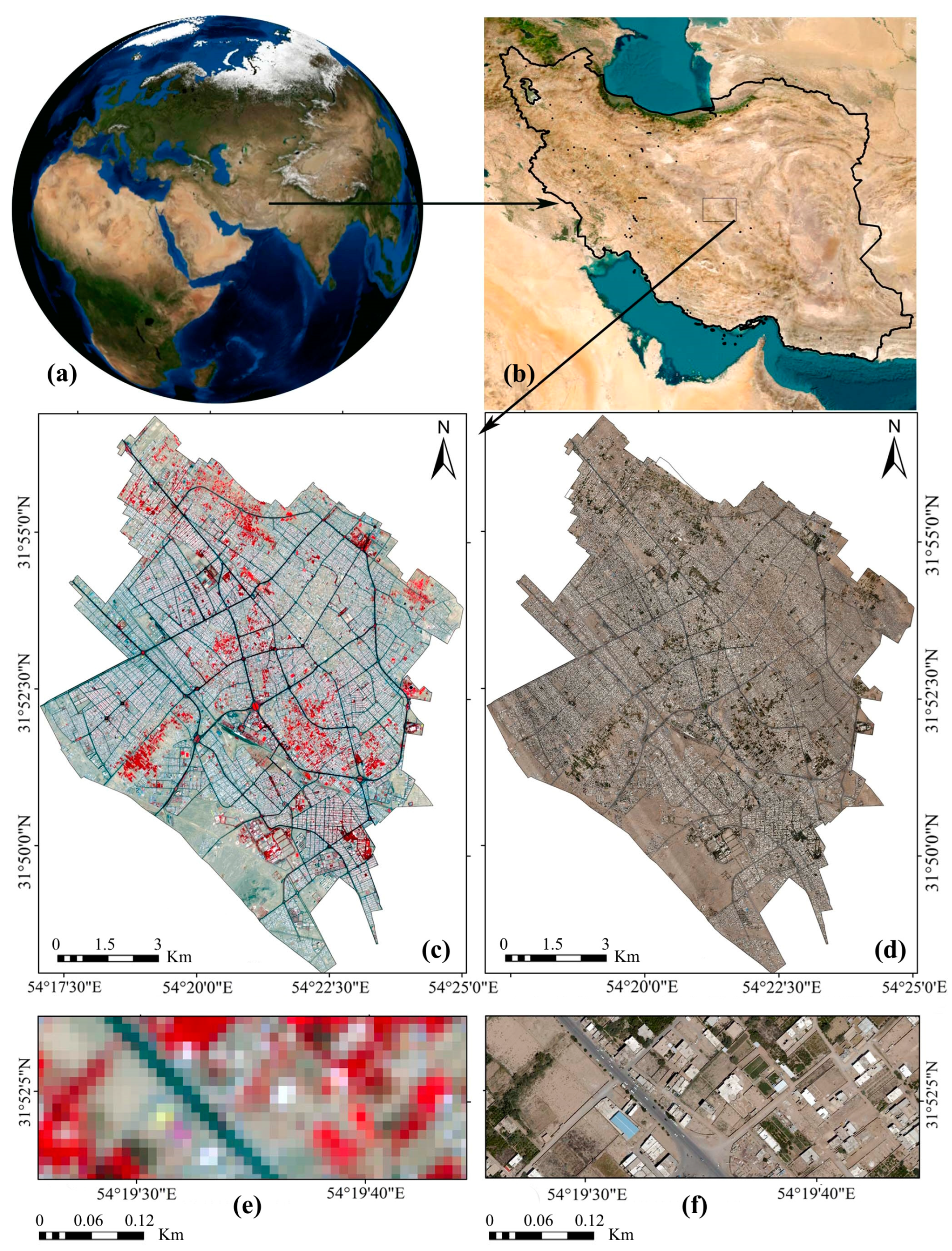
2.1. Study Region

The study area is the entire city of Yazd in Iran. Figure 1 shows this area and a sample of the images used. In terms of geographical location, the studied area is in the center of the province of Yazd between longitude 47°22′54′′ to 33°24′54′′E and latitude 39°47′31′′ to 51°56′31′′N and has an altitude of 1215 m.

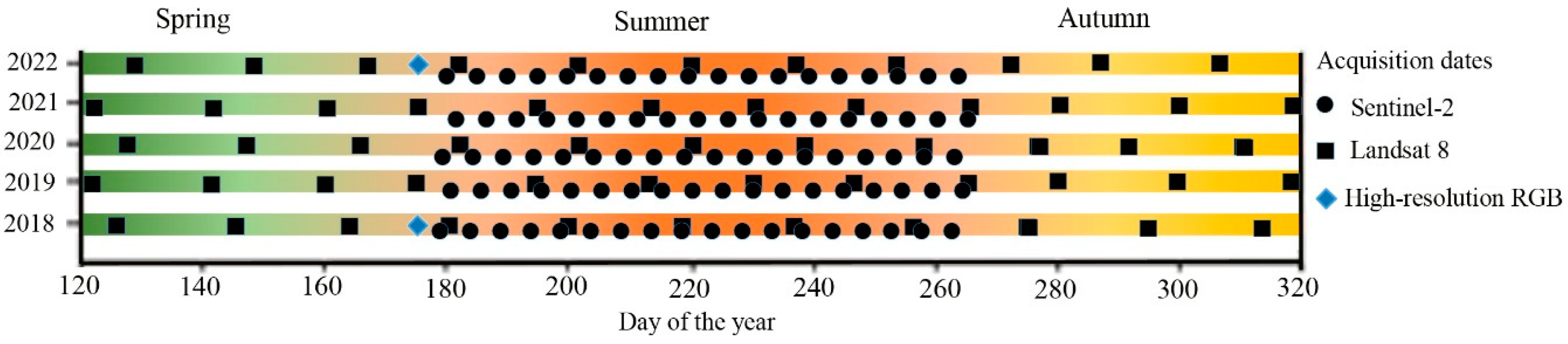
2.2. Datasets and Preprocessing

In this research, Sentinel-2, Landsat 8, and UAV images were used (Figure 2). Landsat 8 was launched in February 2013 as part of the Landsat Data Continuity Mission (LDCM). This satellite carries the Thermal Infrared Sensor (TIRS) and Operational Terrain Imager (OLI). The TIRS can record thermal infrared radiation with a spatial resolution of 100 m with the help of two bands in the atmospheric windows of 10.6 to 11.2 μm for band 10 and 11.5 to 12.5 μm for band 11 [44]. The fact that Landsat 8 is equipped with two thermal bands differentiates it from other Landsat satellites, and this property makes split window algorithms operational for Landsat 8 [45]. These algorithms retrieve the land surface temperature (LST) through the linear integration of the brightness temperature in dual thermal bands [46]. Sentinel-2 is one of the latest multispectral imaging satellites, equipped with the multispectral instrument (MSI), and can record 13 bands [47]. The advantages of using Sentinel-2 images include wide coverage (290 km bandwidth), high spatial resolution (10 m), new spectral qualities (for example, three bands in the red edge plus two bands in the SWIR), and the possibility of obtaining images in a sequence of 5 days. These images have created a useful dataset for applied Earth studies [48]. UAVs are a practical tool for data generation in remote sensing. They can take pictures at any time and place, and they provide images with high spatial resolution, provide the possibility of quick data collection at a low cost and have the possibility of taking images in cloudy conditions [49,50]. Disadvantages and limitations of using drones include the necessary rules and permits before flight, short flight time due to battery limitations, and a large volume of images that require powerful hardware for processing [51,52]. In this research, RGB images with a spatial resolution of 0.15 m were used (aerial images). Because the study area is urban and has a large area, the imaging was performed using the RGB imaging sensor installed on the plane. These cameras have a very limited number of relatively wide spectral bands, but they provide a high spatial resolution at a relatively low cost [53].

2.3. Methods

2.3.1. Sentinel-2 and Aerial Images Fusion

Image fusion creates images with high spatial and spectral resolution. The spectral data of multispectral images are combined with the spatial data of high-resolution images [54,55]. In fusion of images, the imaging time of multispectral images and high-resolution images, such as those obtained from drones, is recommended to be the same or close to each other [56]. In this present study, the ability to fuse Sentinel-2 images and aerial RGB (red-green-blue) images with high spatial resolution was investigated, and eight image fusion methods were compared, including GS, projective, HPF, Brovey, Ehlers, HSC, nearest-neighbor diffusion (NNDiffuse), IHS, color normalization (CN), and wavelet.

The steps in the fusion of multispectral (MS) images with panchromatic (PAN) images in the GS method are as follows:

(1)

Simulating a PAN image from a spectral band with low spatial resolution.

(2)

Applying GS transformation to the simulated PAN image and spectral band, using the simulated PAN band as the first band.

(3)

Replacing the high spatial resolution PAN band with the first band.

(4)

Using GS inverse transformation to create a PAN spectral band [57,58,59].

In the HPF method, a high-pass filter is used to extract the spatial data details of the image with high spatial resolution and then apply those details to the MS image, which involves the following steps:

(1)

Applying the HPF to the PAN image with high spatial resolution.

(2)

Adding the filtered image to each band of the MS image by applying a weighting factor to the standard deviation of the MS bands.

(3)

Matching the histogram of the fused image with the original multispectral image.

The HPF fusion method is based on improving the spatial resolution of the MS image using a high-pass filter which extracts high-frequency data and then applies them to each band of the MS image [60,61].

The IHS fusion method [62,63] has been noticed due to the high spatial resolution of the output image and the high efficiency of this algorithm in satellite imagery [64]. The IHS method is a spectral replacement method that extracts spatial (I) and spectral (H, S) data from a standard RGB image. This method is performed by converting the color space of the MS image from the RGB space to the IHS space and replacing its spatial component with a PAN image, performing the reverse transformation, and returning to the RGB color space [60,65].

The Brovey method is a numerical method in which images are fused by normalizing the values of pixels in the MS image bands and then multiplying them by the values of the corresponding pixels in the PAN image. In this method, addition and multiplication and the ratio between different bands of MS image and PAN image are used [60,66]. The CN method is a developed version of the Brovey method, in which the limitation of the number of bands is removed allowing the user to use images with more than three bands as the input image [67].

The Ehlers method allows the fusion of spectral features and generates a space with minimal color distortion [68]. The underlying idea of this method is to modify the PAN image so that it is like the intensity component of the MS image. This method uses a fast Fourier transform (FFT) filter to partially, rather than entirely, replace the intensity component [69].

The nearest-neighbor diffusion-based method (NNDiffuse) considers each pixel spectrum as a weighted linear combination of the spectra of its neighboring superpixels in the pan-sharpened image. This method uses various factors, such as intensity smoothness (σ), spatial smoothness (${\sigma }_s$), and pixel size ratio to determine PAN intensity [70,71].

The HSC method combines high-resolution PAN data with lower-resolution MS data using the Hyperspherical Color Sharpening algorithm [72]. This approach was designed for the 8-band data of the WorldView-2 sensor but works with any MS data containing three or more bands. In this approach, data are converted from the native color space to HSC. In the first step, it replaces the MS intensity component with an intensity-matched version of the PAN band, and in the next step, it repeats the original MS colors [73].

Projective resolution merge (PRM) is a unique geometric method in which models of PAN and MS images are created with sensor-dependent geometric techniques. Ultimately, these models are fused in such a manner as to preserve the PAN image geometry. The performance of this method based on PAN image filtering is like the HPF method but with different filters [23,74,75]. Principal component analysis (PCA) is a transformation that aims to obtain new components in which the amount of data variance is higher and the dependence between the components is lower than the initial state of the images [76].

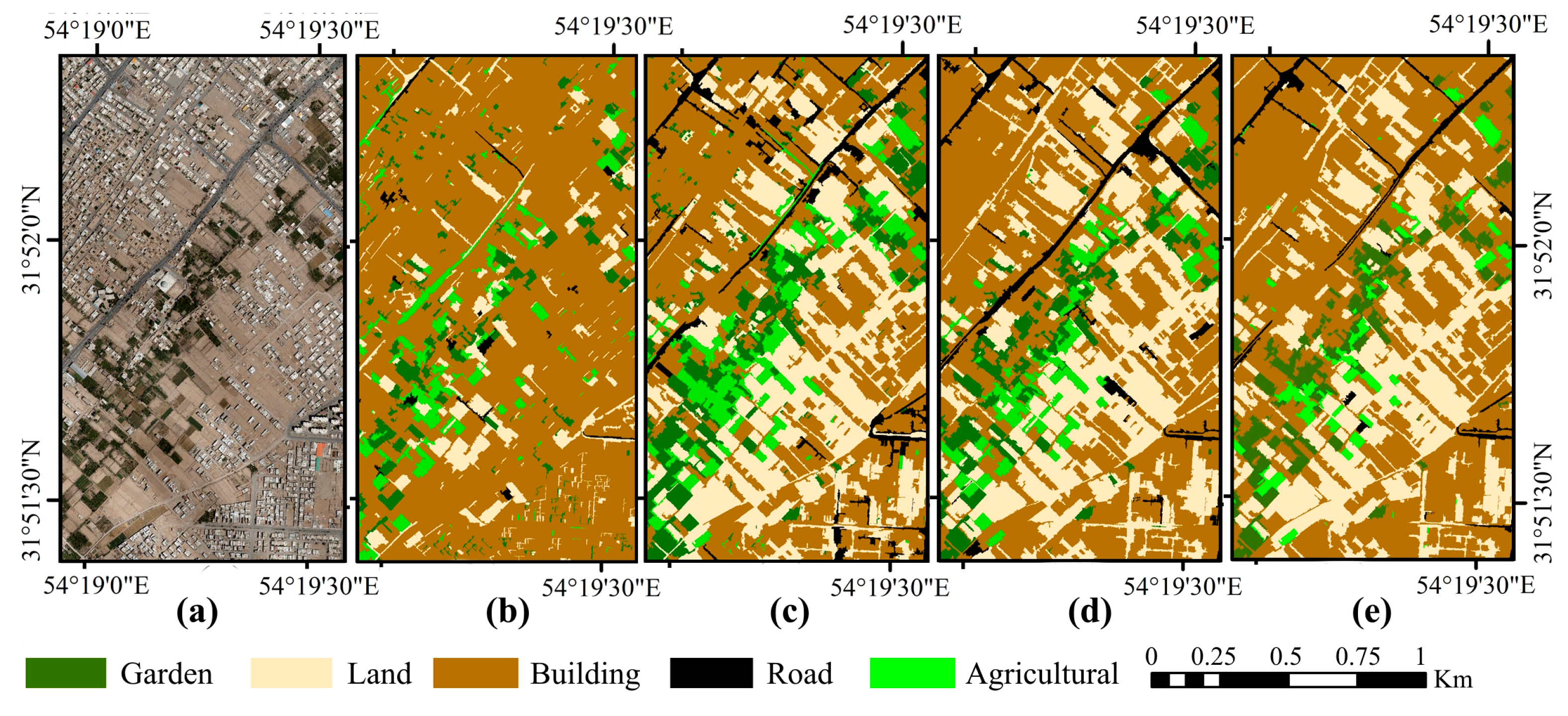
2.3.2. Classification of Images Using Object-Oriented Methods

The use of object-oriented methods in processing satellite images has increased the applicability of environmental remote sensing research [77,78]. In this approach, in addition to numerical values, information related to texture, shape, and color tone is used in the classification process. It has been proven that the ability of the basic pixel classification method is limited when different objects on the ground are recorded with the same numerical values on the digital image. To solve this problem, the object-oriented classification method has been proposed. The most important difference between pixel-based and object-oriented methods is that in object-oriented analysis the main unit of image processing is the shape of objects or segments not the reflective values of individual pixels [79].

Random Forest (RF) is a supervised classification algorithm based on ensemble learning, generated by combining multiple decision trees [80]. The final classification result is obtained by averaging or voting on the results of each decision tree [81]. This method has better performance in dealing with high-dimensional nonlinear classification problems and is widely used in high-resolution image classification [82,83].

SVM is a non-parametric image classification algorithm consisting of a set of related regression and learning classification algorithms [84]. SVM can discriminate between classes by maximizing the gap between classes at the decision level [85,86]. SVM is an algorithm based on statistical learning theory with nonlinear processing capability and high dimensionality and high detection accuracy for small samples [87].

The k-nearest neighbor (KNN) algorithm presented by Wettschereck et al. [88] is an instance-based learning method which classifies elements based on the k-nearest training instances in the source space [89]. In addition to being the main parameters for KNN algorithm adjustment, these data play an important role in spatial prediction. KNN is a nonparametric MLA that makes no assumptions about the original dataset [90]. This is important when classifying change processes in areas where there is little or no prior knowledge of the data distribution [91].

In the Bayes method, the parameters are considered as random variables with a previously known distribution. Also, based on this algorithm, it is assumed that the presence or absence of a special feature of a class is not related to the presence or absence of another feature [92]. In this way, the probability of occurrence of different attribute values for different classes in a training set is estimated by the Bayesian algorithm, and finally these probabilities are used to classify the calling patterns [93]. The results are evaluated based on overall accuracy (OA, kappa coefficient) [94].

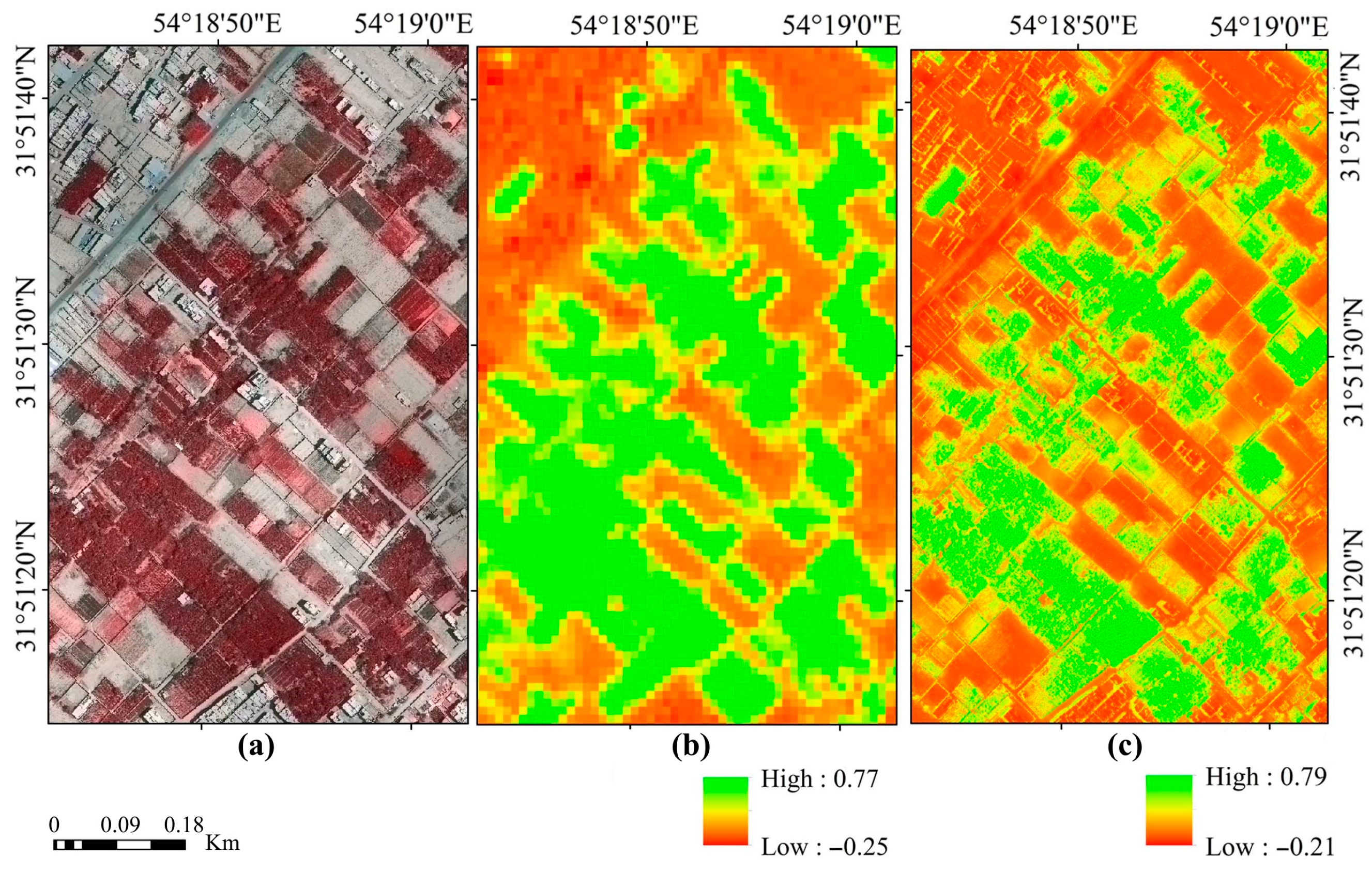
2.3.3. Estimation of Vegetation Index

The reflectance of electromagnetic energy measured in the ultraviolet, visible, and near- and mid-infrared parts of the spectrum is commonly used to generate various vegetation indices that provide useful information about plant structure and condition [95,96]. Preparing a map of these indices helps to understand the spatial-temporal changes in agricultural conditions, which is very useful in precise agriculture [97]. Plant pigments, mainly chlorophyll and carotenoids, are intensively absorbed in the visible part of the spectrum except in the green region. However, such strong absorption does not occur in the NIR part of the spectrum, thus causing high reflectance in the NIR region of green and healthy plants [98,99].

NDVI uses reflectance values measured in the red and NIR regions to provide valuable information about crop growth (LAI, biomass), roots, and photosynthesis. The NDVI value ranges from −1 to 1, where positive values indicate increased greenness and negative values indicate non-vegetated surfaces such as urban areas, soil, bare land, water, and ice [100,101]. NDVI is often used in harmonic analysis because it is a good indicator of vegetation phenology [102]. It is also a suitable index to investigate vegetation changes in time series [103]. The classification of this index and the determination of areas with very good, good, poor, and very poor coverage was determined in a study by Mangewa et al. [104], but in the study area, which has desert conditions and is very poor in terms of vegetation, this classification requires revision, which was determined using a field visit.

2.3.4. Identification of New Construction in Garden Areas

Assessment of the changes which are already occurring is a key factor in environmental monitoring [105]. However, it is not possible to constantly monitor urban areas using drones due to the high costs, problems related to obtaining flight permission, and the large volume of data and processing. In addition, municipalities must prevent unauthorized constructions before the completion of buildings; hence, they need to be aware of the location of constructions. A method has been proposed in previous studies, which allows the identification of new constructions via UAV imaging once a year and using Sentinel-2 images. In this method, a land cover map of the study area is prepared using aerial images and a DSM which is prepared by municipalities at the beginning of every year, through which undeveloped land is identified. The pixel size of the Sentinel-2 images was converted to the size of the aerial images and using the land cover map obtained from the aerial images the undeveloped land was separated on the Sentinel-2 images. Unbuilt lands were checked, and the points that were identified as changes in several consecutive images were determined to be new construction sites. In this way, it is possible to effectively identify new constructions with the lowest cost and time for image processing. The full description of this method is provided in the study by Aliabad et al. [21].

2.3.5. Investigating the Effect of Destruction of Gardens on the LST

According to the results of previous studies in the field of comparing and validating different methods of estimating LST using Landsat 8 images, the split window algorithm has been used [106,107]. To estimate the LST in all methods, it is first necessary to estimate the radiance and brightness temperature (BT) using satellite images using Equation (1):

$$L_{\lambda }=M_L\times Q_{cal}+A_L$$

(1)

where $L_{\lambda }$ is the spectral radiance in the sensor, $M_L$ is the multiplicative conversion factor, $A_L$ is the summation conversion factor, and $Q_{cal}$ is the pixel value of the thermal raw image [108]. Having converted the pixel value to spectral radiance, it is necessary to estimate the BT. The BT can be calculated through the Planck equation and is the actual temperature observed by the satellite under the emissivity theory [109] and Equation (2):

$$\mathrm{B}\mathrm{T}=\frac{K_2}{\ln \left[\left(K_1/L_{\lambda }\right)+1\right]}$$

(2)

The BT is the radiant temperature recorded on the surface of the sensor (in Kelvin), $L_{\lambda }$ is the spectral radiance ($\mathrm{W}\cdot \mathrm{s}{\mathrm{r}}^{-1}\cdot {\mathrm{m}}^{-2}\cdot \mathsf{\mu }{\mathrm{m}}^{-1}$), $K_1$ and $K_2$ are constant values calculated by the effective wavelength received from the satellite sensor. Coefficient values $K_1$ in bands 10 and 11 of Landsat 8 satellite are 774.89 and 480.89 ($\mathrm{W}\mathrm{n}\cdot \mathrm{s}{\mathrm{r}}^{-1}\cdot {\mathrm{m}}^{-2}\cdot \mathsf{\mu }{\mathrm{m}}^{-1}$), respectively, and coefficient values $K_2$ in bands 10 and 11 are 1321.08 K and 1201.14 K, respectively [110]. Emissivity is the ratio of radiation emitted from the surface of an object to the radiation emitted from a black body at the same temperature [111]. To estimate the emissivity from the thermal band of the satellite, the NDVI threshold method was used [112]. The NDVI is estimated using Equation (3):

$$\mathrm{N}\mathrm{D}\mathrm{V}\mathrm{I}=\left(\frac{\mathrm{N}\mathrm{I}\mathrm{R}-\mathrm{R}\mathrm{E}\mathrm{D}}{\mathrm{N}\mathrm{I}\mathrm{R}+\mathrm{R}\mathrm{E}\mathrm{D}}\right)$$

(3)

where NIR and RED are ground reflectance of near infrared and red bands, respectively. NDVI values vary between −1 and +1 [113]. To estimate the emissivity using NDVI, it is necessary to separate NDVI of plant and soil. Areas with NDVI smaller than 0.2 were considered as soil without vegetation ($\mathrm{N}\mathrm{D}\mathrm{V}{\mathrm{I}}_s$) and areas with NDVI greater than 0.2 were considered as vegetation ($\mathrm{N}\mathrm{D}\mathrm{V}{\mathrm{I}}_v$) and fractional vegetation coverage (FVC) was estimated using Equation (4).

$$\mathrm{F}\mathrm{V}\mathrm{C}=\left(\frac{\mathrm{N}\mathrm{D}\mathrm{V}\mathrm{I}-\mathrm{N}\mathrm{D}\mathrm{V}{\mathrm{I}}_s}{\mathrm{N}\mathrm{D}\mathrm{V}{\mathrm{I}}_v+\mathrm{N}\mathrm{D}\mathrm{V}{\mathrm{I}}_s}\right)$$

(4)

where NDVI is calculated for each pixel, and $\mathrm{N}\mathrm{D}\mathrm{V}{\mathrm{I}}_s$ and $\mathrm{N}\mathrm{D}\mathrm{V}{\mathrm{I}}_v$ are NDVI for soil and vegetation, respectively [114].

$$\mathrm{L}\mathrm{S}\mathrm{E}={\epsilon }_s\times \left(1-\mathrm{F}\mathrm{V}\mathrm{C}\right)+{\epsilon }_v\times \mathrm{F}\mathrm{V}\mathrm{C}$$

(5)

The above relationship is used to determine land surface emissivity (LSE), where ${\epsilon }_s$ and ${\epsilon }_v$ are constants for soil and vegetation reflectance coefficients, respectively, and are 0.971 and 0.987, respectively, for Landsat 8 [104,115]. The constant coefficients C in the split window algorithm have been obtained through simulation with different numbers in atmospheric and surface conditions (

Table 1. Numerical values of coefficients in the split window algorithm.

Coefficient	C0	C1	C2	C3	C4	C5	C6
Value	−0/268	1/378	0/183	54/300	−2/238	−129/200	16/400

).

$$\begin{array}{c}{\mathrm{L}\mathrm{S}\mathrm{T}}_{SW9}=\mathrm{B}{\mathrm{T}}_{10}+C_1\left(\mathrm{B}{\mathrm{T}}_{10}-\mathrm{B}{\mathrm{T}}_{11}\right)+C_2(\mathrm{B}{\mathrm{T}}_{10}-\mathrm{B}{\mathrm{T}}_{11}{)}^2+C_0+\\ \left(C_3+C_{4}w\right)(1-m)+(C_5+C_{6}w)\Delta m\end{array}$$

(6)

Parameter $w$ is the amount of atmospheric water vapor column, showing the vertical accumulation of water vapor per unit area with the unit $\left(\mathrm{g}\mathrm{r}\cdot \mathrm{c}{\mathrm{m}}^{-2}\right)$ [45], estimated based on previous studies [115].

$$w=a\left(\frac{{\tau }_j}{{\tau }_i}\right)+b$$

(7)

$$\frac{{\tau }_j}{{\tau }_i}=\frac{{\epsilon }_i}{{\epsilon }_j}{R}_{j,i}$$

(8)

$$R_{j,i}=\frac{{\sum }_{k=1}^N\left(\mathrm{B}{\mathrm{T}}_{10}-\overline{\mathrm{B}{\mathrm{T}}_{10}}\right)\left(\mathrm{B}{\mathrm{T}}_{11}-\overline{\mathrm{B}{\mathrm{T}}_{11}}\right)}{{\sum }_{k=1}^N(\mathrm{B}{\mathrm{T}}_{10}-\overline{\mathrm{B}{\mathrm{T}}_{10}}{)}^2}$$

(9)

$$r^2=\frac{{\left({\sum }_{k=1}^N\left(\mathrm{B}{\mathrm{T}}_{10}-\overline{\mathrm{B}{\mathrm{T}}_{10}}\right)\left(\mathrm{B}{\mathrm{T}}_{11}-\overline{\mathrm{B}{\mathrm{T}}_{11}}\right)\right)}^2}{{\sum }_{k=1}^N{\left(\mathrm{B}{\mathrm{T}}_{10}-\overline{\mathrm{B}{\mathrm{T}}_{10}}\right)}^2{\sum }_{k=1}^N{\left(\mathrm{B}{\mathrm{T}}_{11}-\overline{\mathrm{B}{\mathrm{T}}_{11}}\right)}^2}=R_{i,j}{R}_{j,i}$$

(10)

In the above equations, $\mathrm{B}{\mathrm{T}}_{10}$ and $\mathrm{B}{\mathrm{T}}_{11}$ are the brightness temperature of bands 10 and 11, τ is the atmospheric transfer coefficient, and a and b are constant coefficients which have been considered as −13.41 and 14.15, respectively [116]. Figure 3 shows the general steps of the research.

3. Results

3.1. Comparison of Fusion Methods

In the present study, in order to separate garden lands from agricultural land and to monitor the condition of vegetation in garden lands, it was necessary to use UAV images, because satellite images with medium spatial resolution, such as Sentinel-2 images with a spatial resolution of 10 m, do not have the ability to accurately separate garden lands. Since the studied area is a city, it was not possible to take pictures of the entire area with multispectral UAV images due to high costs and being time-consuming; hence, RGB images prepared using cameras installed on airplanes (aerial images) and Sentinel-2 satellite images were fused. Fusion of the aerial and Sentinel-2 images was carried out to obtain images with high spatial and spectral resolution. Various methods for the fusion of satellite images and high-resolution RGB images (aerial photos) including Gram–Schmidt, projective, HPF, Brovey, Ehlers, HSC, NNDiffuse, IHS, CN, and wavelet were examined. A comparison between aerial images and images obtained from Sentinel-2 with images fused using different methods is presented in Figure 4 using false color combination.

An important issue in image fusion is evaluating the quality of the integrated image, so that spatial data are improved by preserving spectral data. The correlation coefficient (CC), root mean square error (RMSE) and erreur relative globale adimensionnelle de synthèse (ERGAS) statistical coefficients were used to compare the accuracy of different image fusion methods (

Table 2. The values of statistical coefficients between the corresponding bands in the fused images and the bands of the Sentinel-2 images.

	Brovey	IHS	Ehlers	HPF	GS	PRM	CN	NNDiffuse	HSC	PSC
CC	0/92	0.97	0.97	0.88	0.97	0.94	0.86	0.96	0.91	0.96
RMSE	14.61	13.5	12.3	15.1	13.5	13.82	17.5	13.8	18.37	13.79
ERGAS	1.97	1.87	1.73	2.39	1.73	2.16	2.61	1.95	2.37	1.98

). The results show that the examined methods perform almost identically in terms of preserving the spatial data in the fusion outcome, but they have different results in terms of spectrum. Therefore, the image fusion method is selected according to the different applications and the type of data required, either spectral or spatial. The results of our analyses showed that CC was estimated to be greater than 0.86 in all the methods; even greater than 0.9 except for the CN and HPF methods where the correlation coefficient was 0.86 and 0.88, respectively. Also, in the case of the Ehlers, IHS, and Gram–Schmidt methods, the value of the correlation coefficient was estimated to be 0.97. This statistical coefficient showed relatively similar results in some methods and alone is not a suitable criterion for comparing methods. The results of RMSE analysis of different image fusion methods showed that the HSC and CN methods had the highest error coefficient with RMSE values of 18.37 and 17.5, respectively; also that the Ehlers method yielded the highest accuracy with RMSE of 12.3, followed by IHS and GS with RMSE 13.5 and NNDiffuse and PSC with RMSE 13.8. Comparison of the ERGAS parameter, which is sensitive to mean displacement and dynamic rate change, showed that this parameter was estimated to be smaller than 2.6 in all methods. In fact, in the case of the CN, HPF, HSC, and PRM methods, the value of ERGAS was calculated to be 2.6, 2.4, 2.37, and 2.16, respectively, and in the rest of the methods, this component was smaller than 2. Moreover, comparisons showed that the smallest values of ERGAS were obtained with GS, Ehlers, and IHS, which were estimated to be 1.73, 1.73, and 1.87, respectively. In general, by comparing different coefficients and according to the purpose of the research, which is to preserve both spectral and spatial qualities together, the Ehlers method was used for the fusion of aerial and Sentinel-2 images. For comparison, the NDVI index obtained from Sentinel-2 and the images obtained by fusion of aerial images with Sentinel-2 is shown in Figure 5.

3.2. Comparison of Object-Oriented Classification Methods

To classify the images and separate the gardens from agricultural lands, UAV images, DSM, and NDVI obtained from the fusion of aerial images and Sentinel-2 images were used. The DSM image, which is a raster layer whose value per pixel is equal to the height of natural features and man-made features such as cities and electric lights, adds height information to improve classification. Moreover, the NDVI obtained from the fusion of the UAV image and Sentinel-2 images can improve the classification accuracy by improving the spectral data of the images as well as the difference in the value of the vegetation index and its reflection in the red and infrared bands. According to previous studies in the field of comparing object-oriented and pixel-based methods [117], object-oriented methods were selected for classification.

In the first stage of classification, using various optimization techniques, the most suitable scale and parameters involved in the classification were identified, then in the next stage, according to the scale and power of spatial separation of the image, segmentation of the image components was carried out, and finally, complications were classified using the desired technique. In the case of object-oriented classifications of satellite images, the quality of segmentation and determining the scale of segments have a direct relationship with the power of spatial separation of satellite images, and by increasing the spatial separation of images, high-quality segments can be produced, and the accuracy of classification can be significantly increased.

The process of object-oriented classification can be conducted in three general stages, which include segmentation, classification, and evaluation of classification accuracy. A segment means a group of neighboring pixels within an area, where similarities such as numerical value and texture are the most important common criteria. Image objects resulting from the segmentation process are the basis of object-oriented classification. For the purpose of segmentation in this research, the multi-resolution segmentation method has been used. Since in the current study the purpose of classification is to separate garden lands from agricultural lands, a segment that can best put garden lands into one category is desirable.

To conduct different tests for segmentation, various parameter scales were used, including 100, 50, and 30. A parameter comparison that can provide segments with the dimensions of garden and agricultural land is desirable, and according to the purpose of the research, there is no need for segmentation on the scale of each tree or crop rows. Therefore, the visual examination of the three abovementioned tests showed that the parameter scale of 50 was most suitable for the segmentation of garden lands in this image, and then the optimal coefficient values of the image and compression factor were selected to be 0.4 and 0.5, via trial and error (Figure 6). The segments were created in such a way that the agricultural lands are separated as a segment. After applying image segmentation, classification was carried out using Bayesian object-oriented methods, RF, SVM, and KNN, the results of which are presented in Figure 7.

In the present study, the DSM image and NDVI were used to increase the accuracy of aerial image classification. The DSM image by adding height information and NDVI by adding spectral information of complications help to separate gardens from agricultural fields. In the classification using the Bayes method, building land cover, and bare lands have not been appropriately separated from each other, and the roads are not identified at all and the land is classified as buildings; hence, from a visual point of view, this method does not have the ability to distinguish different land covers. The KNN and RF methods have moderate accuracy and the SVM method has better distinguished different land covers. In fact, SVM outperforms other methods in terms of separation of different land covers, especially roads. The criteria used for evaluation were the overall accuracy and kappa coefficients. Because it considers the agreement that would be predicted by chance, the kappa coefficient is a more reliable indicator than the total accuracy metric. The results of comparing the kappa coefficient and overall accuracy of different object-oriented classification methods (

Table 3. Comparison of the accuracy of aerial images classification methods in distinguishing gardens from agricultural lands.

	Kappa Coefficient	Overall Accuracy
SVM	89%	86.2
Bayes	58%	51.3
KNN	76%	81.4
RF	87%	83.1

) indicated that SVM has the highest accuracy with kappa coefficient and overall accuracy of 0.89 and 86.2, respectively; followed by the random forest method with a kappa coefficient and overall accuracy of 0.87 and 83.1. The Bayes method has the lowest accuracy with a kappa coefficient of 0.58. The object-oriented methods used in this research, from the most to the least accurate, include SVM, RF, KNN, and Bayes. Therefore, the SVM method was used to classify aerial images in this research [21].

3.3. Monitoring the State of Vegetation in Gardens

Having separated garden lands in the images of 2018, in order to examine the vegetation status of the gardens at the present time, the aerial images of this year were again fused with the Sentinel-2 images and the NDVI was calculated. NDVI values were classified into four groups including dried, drying, acceptable, and desirable conditions (very poor, poor, good, and very good) (Figure 8). Since the studied region has a dry climate and desert conditions, NDVI classification was carried out by field visits in several gardens, and its values are different from the classifications considered for humid areas (

Table 4. The classification values of NDVI for dry areas in the present study.

NDVI	Name	Color	Class
0.4<	Desirable conditions		Very Good
0.3–0.4	Acceptable conditions		Good
0.2–0.3	Drying up		Poor
0.2>	Dried		Very Poor

). The NDVI threshold was determined by dividing the state of trees into four states, which was done by using a review of sources in this field and then a field visit, an example of which is shown in Figure 9.

Through the classification of images and the separation of gardens from agricultural lands in 2018, it turned out that there are 1258 gardens covered with trees in the study area. Since lands with an area of less than 500 square meters are not considered as gardens, the number of gardens in the study area is 1024. The percentage of each garden status class in each garden was calculated for 2022 and the results showed that 21 gardens have completely dried up in the period under study and the NDVI in the entire area of these gardens during the peak vegetation cover in summer is smaller than 0.2. Also, in 17 gardens between 70 and 90% of the area and in 44 gardens between 50 and 70% of the area have dried up. In order to more comprehensively examine the state of the gardens, the percentage of each class of dried, drying, acceptable, and desirable conditions was divided into five categories, which comprise 0 to 20, 20 to 40, 40 to 60, 60 to 80, and above 80 percent. In each garden status class, the frequency of these categories was determined (Figure 10). The results of the examination of the percentage of the area in different classes of gardens showed that 786 gardens have less than 20%, 129 gardens between 20 and 40%, 60 gardens between 40 and 60%, and 49 gardens more than 60% of their area in the completely dried class. In other words, in 24% of the gardens in the study area, equivalent to 238 gardens, more than 20% of their area has completely dried up in the period between 2018 and 2022.

Examining the status class ‘drying’ showed that 618 gardens have less than 20% of their area in this class. Also, in 38 gardens, more than 80% of the garden area is drying up. In 71 gardens in the study area, more than 60% of the garden area is drying up. These gardens will be prioritized for restoration and if their problem is a lack of water resources, they will be irrigated by organizations such as the municipality or the urban green space organization.

The results of examining the status class ‘acceptable’ also showed that 200 gardens have more than 40% of their area in this category. Examination of the status class ‘desirable’ showed that 340 gardens (34% of the gardens in the study area) have less than 20% of their area in desirable condition. Also, from the entire studied area, 100 gardens have more than 80% of their area in good condition. Due to the ideal vegetation, these gardens can be invested in by the municipality and purchased to become public green spaces.

It is necessary to plan for different categories of gardens according to the mentioned statistics in order to prevent further drying of gardens. The percentage of vegetation status classes in each garden was also compared with its area, and the results showed that gardens with a small area were more prone to destruction (Figure 11). Completely dried conditions are more common in gardens with a small area, and there are more desirable vegetation conditions in gardens with a large area.

3.4. Identification of New Construction in Gardens

Through the examination of the changes in Sentinel-2 images, new constructions were identified in the gardens in the time series from 2018 to 2022 and were compared with the aerial images taken in 2022. The results showed that 108 new construction locations were identified using Sentinel-2 images, while 120 new construction locations were identified using UAV images. In general, during the times when it is not possible to obtain images with high spatial resolution, Sentinel-2 images and their monitoring over time make it possible to identify new constructions. Figure 12 illustrates an example of the destruction of gardens followed by new constructions. With an area of 6000 square meters in 2018, this garden had been converted into 17 residential buildings by 2022. Effective and in-time identification of the location of new constructions in garden lands is very crucial to prevent and legally deal with their change of use and can prevent further destruction of gardens. Therefore, the use of Sentinel-2 images and their monitoring in a time series to identify new constructions in gardens makes it possible to give early warning to the relevant authorities and prevent the destruction of gardens and their illegal change of use.

3.5. Investigating the Effect of the Garden Destruction on the LST

Having identified the destroyed gardens, the effects of the destruction of gardens and the change in the land cover of the gardens on LST were examined. The LST is a variable which significantly varies with time and space; hence, checking LST on one day of two different years is not a correct method to identify the effects of changes in land cover on the LST. For this purpose, in the current study, the LST was estimated using the split window algorithm and Landsat 8 images in a five-year time series from 2018 to 2022 with a sequence of 16 days (125 images of LST). Given that satellite images are always associated with the problem of clouds and missing data, and due to the necessity of obtaining a complete time series to examine the changes in the time series of the LST, these images were reconstructed using the HANTS algorithm, and the outlier data caused by clouds and snow were estimated. This algorithm has been examined in previous studies on reconstructing the LST images of Landsat 8 [118]. Changes in the LST have been examined in a five-year time series in a garden that had a constant status, a garden that has been destroyed in the past two years, and on land without vegetation (Figure 13).

The results of monitoring LST in a five-year time series showed that there was no change in the conditions of the vegetation in the garden during the given period. The pattern of changing LST has also been constant and the maximum temperature in summer in this garden is 38 °C and the minimum temperature in the cold months of the year is 10 °C. The LST in a land without vegetation is estimated to be over 50 °C in summer and up to 15 °C in winter. Therefore, there is a significant difference between the pattern of LST changes in garden lands and lands without vegetation, and this temperature difference is much greater in the hot seasons of the year. Hence, in summer, the temperature difference between gardens and bare land is 20 °C while it is less than 10 °C in winter. The pattern of changes in LST of the studied destroyed garden from 2018 to 2020 is completely identical to the garden with desirable coverage, and in 2021 and 2020 its temperature increased significantly, which indicates the complete destruction of the vegetation. The maximum LST in the summer before the destruction of the garden was 38 °C while it was 52 °C after the destruction. Therefore, destroying the vegetation in this garden has increased the surface temperature by 14 °C.

To investigate the effect of the drying of the gardens on the increase in LST, the changes in LST between the dried gardens and the gardens with desirable tree cover were also compared, in addition to the changes over time which were examined in the previous section, to determine the spatial changes of the surface temperature between the land with desirable vegetation and the dried gardens. The LST was checked in the summer of 2022 in the lands that had once been identified as gardens in 2018, and the results are shown in two plots as an example in Figure 14. As is clear in this figure, the gardens that have dried up in the studied time series have a much higher LST than the gardens with desirable conditions. Maximum LST in gardens with desirable conditions is 38 °C and is 44 °C in dried gardens; also, average LST in desirable gardens is 36.2 °C while it is 42.5 °C in dried gardens. Since the spatial resolution of Landsat 8 surface temperature images is 100 m, the problem of mixed pixels has caused temperature changes to be unclear in small gardens or gardens that have only been partially destroyed.

4. Discussion

Comparing the results of this research with previous studies shows that the results of selecting the optimal method for fusion of UAV images with Sentinel-2 are in line with the results of Ai et al. [119] demonstrating that the Ehlers, IHS, Mojak, and Gram–Schmidt methods have the highest to the lowest accuracy in image fusion. In the present study, the accuracy of the Ehlers method was higher than the other three methods. However, the results were incompatible with the results of the study by Rahimzadeganasl et al. [120], who showed that Gram–Schmidt, NNDiffuse, and IHS methods are more accurate than the Ehlers and HSC methods. The results of the present study showed that the mentioned methods are more accurate than the HSC method, but their accuracy is lower than the Ehlers method.

The results of the present study are also in line with the results of Li et al. [23] who found the value of the correlation coefficient in the PSC and Brovey methods to be lower than that of Ehlers. Also, the results of the current research are in line with the study of Moltó [31] which used the fusion of RGI high resolution images and Sentinel-2. It is possible to prepare the NDVI with high accuracy and distinguish different land covers because, in this study, the capability of RGB high resolution images in this field was also confirmed. The results of using the DSM image to increase classification accuracy are consistent with the results of Al-Najjar et al. [121] indicating that the use of a DSM has the greatest effect on improving the accuracy of identifying trees and buildings. The present study also confirms the results of Beltrán-Marcos et al. [29] arguing that the use of a DSM increases the accuracy of classification and segmentation. The results of the present study showed that the use of NDVI image spectral data along with a DSM increases the accuracy of aerial image classification, which is consistent with the results of Wu et al. [17]. Also, the results of comparing various classification methods using the object-oriented method are in line with the results of Marcinkowska et al. [122] and Burai et al. [123] which stated that the SVM method provides the flexibility of training data, thus reducing errors and increasing accuracy. It also confirms the results of Bento et al. [124] who found the SVM and RF methods to be the most appropriate methods for preparing land use maps in agricultural areas. The results of Zhang [125] showed that spectral information from the fusion of multispectral aerial imagery can be used for machine learning-based land cover classification, and among all methods, SVM had the best performance, which confirms the results of the present study.

The limitations of the current research include the following. Using aerial images with high spatial resolution requires powerful hardware and its processing is very time-consuming. Aerial images in some areas may not be available at local noon time. Therefore, a shadow is created in the images, and the presence of a shadow in the classification causes a partial error. The advantage of this research is that due to the location of the studied area in the desert and hot and dry climate, the results of this study can help to preserve and prevent the destruction of existing gardens. Also, the gardens that are drying out have been identified and irrigated to prevent them from drying out. The fusion of aerial images and Sentinel-2 led to a more accurate monitoring of the state of vegetation in dry areas.

5. Conclusions

Traditional methods to identify garden lands and monitor their vegetation status (including field surveys) are associated with inevitable disadvantages. For example, these methods are unusable in areas which are not easily accessible, and are also laborious, expensive, and challenging in other areas. Therefore, the use of remote sensing, which is freely available to the public with a time sequence, is a suitable method for this type of study. As drone technology continues to improve, the costs and obstacles of drone operations are falling, and the use of related technology in agriculture has become common. Reducing the number of workers in the agricultural industry makes UAV technology an effective tool for agricultural land management by local governments and academic research to promote precision agriculture, which focuses on high efficiency, food safety, and risk prevention. In the present study, satellite and aerial images were fused using different methods. In fusion of satellite images, the important issue is the amount of preserving spectral data while simultaneously increasing spatial data. Using the optimal method, the images were fused and the vegetation index was estimated. In this study, aerial images and the vegetation index obtained by fusion of UAV and Sentinel-2 images were used to classify and separate garden and agricultural lands. The results showed that the proposed method effectively increases the classification accuracy. Comparison of various object-oriented classification methods showed that the use of the SVM method can distinguish gardens from other land covers, especially agricultural lands, with appropriate accuracy. Monitoring the condition of the vegetation in the study area, which is a city with a dry climate and desert conditions, showed that the gardens in the study area were extensively destroyed and 120 buildings were built inside the gardens during the study period. Also, the results showed that the destruction of gardens caused a sharp increase in LST. Considering the lack of green space in the study area, it is very crucial to preserve and monitor the gardens to prevent their destruction and drying. It is also suggested to use a Markov chain to predict the state of gardens in the coming years.

References

1. Mirzaee, S.; Mirzakhani Nafchi, A. Monitoring Spatiotemporal Vegetation Response to Drought Using Remote Sensing Data. Sensors 2023, 23, 2134. [Google Scholar] [CrossRef] [PubMed]
2. Ghaderpour, E.; Mazzanti, P.; Scarascia Mugnozza, G.; Bozzano, F. Coherency and phase delay analyses between land cover and climate across Italy via the least-squares wavelet software. Int. J. Appl. Earth Obs. Geoinf. 2023, 118, 103241. [Google Scholar] [CrossRef]
3. Liu, Z.; Chen, D.; Liu, S.; Feng, W.; Lai, F.; Li, H.; Zou, C.; Zhang, N.; Zan, M. Research on Vegetation Cover Changes in Arid and Semi-Arid Region Based on a Spatio-Temporal Fusion Model. Forests 2022, 13, 2066. [Google Scholar] [CrossRef]
4. Ghorbanian, A.; Mohammadzadeh, A.; Jamali, S. Linear and Non-Linear Vegetation Trend Analysis throughout Iran Using Two Decades of MODIS NDVI Imagery. Remote Sens. 2022, 14, 3683. [Google Scholar] [CrossRef]
5. Almalki, R.; Khaki, M.; Saco, P.M.; Rodriguez, J.F. Monitoring and Mapping Vegetation Cover Changes in Arid and Semi-Arid Areas Using Remote Sensing Technology: A Review. Remote Sens. 2022, 14, 5143. [Google Scholar] [CrossRef]
6. Kellert, A.; Bremer, M.; Low, M.; Rutzinger, M. Exploring the potential of land surface phenology and seasonal cloud free composites of one year of Sentinel-2 imagery for tree species mapping in a mountainous region. Int. J. Appl. Earth Obs. Geoinf. 2021, 94, 102208. [Google Scholar] [CrossRef]
7. Lindberg, E.; Holmgren, J.; Olsson, H. Classification of tree species classes in a hemi-boreal forest from multispectral airborne laser scanning data using a mini raster cell method. Int. J. Appl. Earth Obs. Geoinf. 2021, 100, 102334. [Google Scholar] [CrossRef]
8. Modzelewska, A.; Fassnacht, F.E.; Sterenczak, K. Tree species identification within an extensive forest area with diverse management regimes using airborne hyperspectral data. Int. J. Appl. Earth Obs. Geoinf. 2020, 84, 101960. [Google Scholar] [CrossRef]
9. Grabska, E.; Hostert, P.; Pflugmacher, D.; Ostapowicz, K. Forest stand species mapping using the Sentinel-2-time series. Remote Sens. 2019, 11, 1197. [Google Scholar] [CrossRef]
10. Wang, M.; Zheng, Y.; Huang, C.; Meng, R.; Pang, Y.; Jia, W.; Zhou, J.; Huang, Z.; Fang, L.; Zhao, F. Assessing Landsat-8 and Sentinel-2 spectral-temporal features for mapping tree species of northern plantation forests in Heilongjiang Province, China. For. Ecosyst. 2022, 9, 100032. [Google Scholar] [CrossRef]
11. Madonsela, S.; Cho, M.A.; Mathieu, R.; Mutanga, O.; Ramoelo, A.; Kaszta, Z.; Van De Kerchove, R.; Wolff, E. Multi-phenology WorldView-2 imagery improves remote sensing of savannah tree species. Int. J. Appl. Earth Obs. Geoinf. 2017, 58, 65–73. [Google Scholar] [CrossRef]
12. Rahman, M.F.F.; Fan, S.; Zhang, Y.; Chen, L. A comparative study on application of unmanned aerial vehicle systems in agriculture. Agriculture 2022, 11, 22. [Google Scholar] [CrossRef]
13. Ahmadi, P.; Mansor, S.; Farjad, B.; Ghaderpour, E. Unmanned Aerial Vehicle (UAV)-Based Remote Sensing for Early-Stage Detection of Ganoderma. Remote Sens. 2022, 14, 1239. [Google Scholar] [CrossRef]
14. Grybas, H.; Congalton, R.G. A comparison of multi-temporal RGB and multispectral UAS imagery for tree species classification in heterogeneous New Hampshire Forests. Remote Sens. 2021, 13, 2631. [Google Scholar] [CrossRef]
15. Belcore, E.; Pittarello, M.; Lingua, A.M.; Lonati, M. Mapping riparian habitats of natura 2000 network (91E0*, 3240) at individual tree level using UAV multi-temporal and multi-spectral data. Remote Sens. 2021, 13, 1756. [Google Scholar] [CrossRef]
16. Johansen, K.; Duan, Q.; Tu, Y.H.; Searle, C.; Wu, D.; Phinn, S.; Robson, A.; McCabe, M.F. Mapping the condition of macadamia tree crops using multi-spectral UAV and WorldView-3 imagery. ISPRS J. Photogramm. Remote Sens. 2020, 165, 28–40. [Google Scholar] [CrossRef]
17. Wu, Q.; Zhang, Y.; Xie, M.; Zhao, Z.; Yang, L.; Liu, J.; Hou, D. Estimation of Fv/Fm in spring wheat using UAV-Based multispectral and RGB imagery with multiple machine learning methods. Agronomy 2023, 13, 1003. [Google Scholar] [CrossRef]
18. Hegarty-Craver, M.; Polly, J.; O’Neil, M.; Ujeneza, N.; Rineer, J.; Beach, R.H.; Temple, D.S. Remote crop mapping at scale: Using satellite imagery and UAV-acquired data as ground truth. Remote Sens. 2020, 12, 1984. [Google Scholar] [CrossRef]
19. Shamshiri, R.R.; Hameed, I.A.; Balasundram, S.K.; Ahmad, D.; Weltzien, C.; Yamin, M. Fundamental research on unmanned aerial vehicles to support precision agriculture in oil palm plantations. In Agricultural Robots-Fundamentals and Applications; IntechOpen: London, UK, 2018; pp. 91–116. [Google Scholar]
20. Yuan, L.; Zhu, G. Research on Remote Sensing Image Classification Based on Feature Level Fusion. ISPRS—Int. Arch. Photogramm. Remote Sens. Spat. Inf. Sci. 2018, XLII-3, 2185–2189. [Google Scholar] [CrossRef]
21. Aliabad, F.A.; Malamiri, H.R.G.; Shojaei, S.; Sarsangi, A.; Ferreira, C.S.S.; Kalantari, Z. Investigating the Ability to Identify New Constructions in Urban Areas Using Images from Unmanned Aerial Vehicles, Google Earth, and Sentinel-2. Remote Sens. 2022, 14, 3227. [Google Scholar] [CrossRef]
22. Jenerowicz, A.; Woroszkiewicz, M. The pan-sharpening of satellite and UAV imagery for agricultural applications. In Remote Sensing for Agriculture, Ecosystems, and Hydrology XVIII; Neale, C.M.U., Maltese, A., Eds.; SPIE: Bellingham, WA, USA, 2016; Volume 9998. [Google Scholar]
23. Li, Y.; Yan, W.; An, S.; Gao, W.; Jia, J.; Tao, S.; Wang, W. A Spatio-Temporal Fusion Framework of UAV and Satellite Imagery for Winter Wheat Growth Monitoring. Drones 2023, 7, 23. [Google Scholar] [CrossRef]
24. Lu, T.; Wan, L.; Qi, S.; Gao, M. Land Cover Classification of UAV Remote Sensing Based on Transformer—CNN Hybrid Architecture. Sensors 2023, 23, 5288. [Google Scholar] [CrossRef] [PubMed]
25. Alvarez-Vanhard, E.; Corpetti, T.; Houet, T. UAV & satellite synergies for optical remote sensing applications: A literature review. Sci. Remote Sens. 2021, 3, 100019. [Google Scholar]
26. Navarro, J.A.; Algeet, N.; Fernández-Landa, A.; Esteban, J.; Rodríguez-Noriega, P.; Guillén-Climent, M.L. Integration of UAV, Sentinel-1, and Sentinel-2 data for mangrove plantation aboveground biomass monitoring in Senegal. Remote Sens. 2019, 11, 77. [Google Scholar] [CrossRef]
27. Yilmaz, V.; Gungor, O. Fusion of very high-resolution UAV images with criteria-based image fusion algorithm. Arab. J. Geosci. 2016, 9, 59. [Google Scholar] [CrossRef]
28. Zhao, L.; Shi, Y.; Liu, B.; Hovis, C.; Duan, Y.; Shi, Z. Finer classification of crops by fusing UAV images and Sentinel-2A data. Remote Sens. 2019, 11, 3012. [Google Scholar] [CrossRef]
29. Beltrán-Marcos, D.; Suárez-Seoane, S.; Fernández-Guisuraga, J.M.; Fernández-García, V.; Marcos, E.; Calvo, L. Relevance of UAV and sentinel-2 data fusion for estimating topsoil organic carbon after forest fire. Geoderma 2023, 430, 116290. [Google Scholar] [CrossRef]
30. Daryaei, A.; Sohrabi, H.; Atzberger, C.; Immitzer, M. Fine-scale detection of vegetation in semi-arid mountainous areas with focus on riparian landscapes using Sentinel-2 and UAV data. Comput. Electron. Agric. 2020, 177, 105686. [Google Scholar] [CrossRef]
31. Moltó, E. Fusion of different image sources for improved monitoring of agricultural plots. Sensors 2022, 22, 6642. [Google Scholar] [CrossRef]
32. Bolyn, C.; Lejeune, P.; Michez, A.; Latte, N. Mapping tree species proportions from satellite imagery using spectral-spatial deep learning. Remote Sens. Environ. 2022, 280, 113205. [Google Scholar] [CrossRef]
33. De Giglio, M.; Greggio, N.; Goffo, F.; Merloni, N.; Dubbini, M.; Barbarella, M. Comparison of pixel-and object-based classification methods of unmanned aerial vehicle data applied to coastal dune vegetation communities: Casal borsetti case study. Remote Sens. 2019, 11, 1416. [Google Scholar] [CrossRef]
34. Phiri, D.; Simwanda, M.; Salekin, S.R.; Nyirenda, V.; Murayama, Y.; Ranagalage, M. Sentinel-2 Data for Land Cover. Use Mapping: A Review. Remote Sens. 2020, 12, 2291. [Google Scholar] [CrossRef]
35. Zhen, Z.; Chen, S.; Yin, T.; Gastellu-Etchegorry, J.P. Improving Crop Mapping by Using Bidirectional Reflectance Distribution Function (BRDF) Signatures with Google Earth Engine. Remote Sens. 2023, 15, 2761. [Google Scholar] [CrossRef]
36. Tarantino, C.; Forte, L.; Blonda, P.; Vicario, S.; Tomaselli, V.; Beierkuhnlein, C.; Adamo, M. Intra-annual sentinel-2 time-series supporting grassland habitat discrimination. Remote Sens. 2021, 13, 277. [Google Scholar] [CrossRef]
37. Kluczek, M.; Zagajewski, B.; Kycko, M. Airborne HySpex hyperspectral versus multitemporal Sentinel-2 images for mountain plant communities mapping. Remote Sens. 2022, 14, 1209. [Google Scholar] [CrossRef]
38. Kluczek, M.; Zagajewski, B.; Zwijacz-Kozica, T. Mountain Tree Species Mapping Using Sentinel-2, PlanetScope, and Airborne HySpex Hyperspectral Imagery. Remote Sens. 2023, 15, 844. [Google Scholar] [CrossRef]
39. Praticò, S.; Solano, F.; Di Fazio, S.; Modica, G. Machine learning classification of mediterranean forest habitats in google earth engine based on seasonal sentinel-2 time-series and input image composition optimisation. Remote Sens. 2021, 13, 586. [Google Scholar] [CrossRef]
40. Liu, X.; Liu, H.; Datta, P.; Frey, J.; Koch, B. Mapping an invasive plant Spartina alterniflora by combining an ensemble one-class classification algorithm with a phenological NDVI time-series analysis approach in middle coast of Jiangsu, China. Remote Sens. 2020, 12, 4010. [Google Scholar] [CrossRef]
41. Bollas, N.; Kokinou, E.; Polychronos, V. Comparison of sentinel-2 and UAV multispectral data for use in precision agriculture: An application from northern Greece. Drones 2021, 5, 35. [Google Scholar] [CrossRef]
42. Maimaitijiang, M.; Sagan, V.; Sidike, P.; Daloye, A.M.; Erkbol, H.; Fritschi, F.B. Crop monitoring using satellite/UAV data fusion and machine learning. Remote Sens. 2020, 12, 1357. [Google Scholar] [CrossRef]
43. Chen, P.C.; Chiang, Y.C.; Weng, P.Y. Imaging using unmanned aerial vehicles for agriculture land use classification. Agriculture 2020, 10, 416. [Google Scholar] [CrossRef]
44. Wulder, M.A.; White, J.C.; Loveland, T.R.; Woodcock, C.E.; Belward, A.S.; Cohen, W.B.; Fosnight, E.A.; Shaw, J.; Masek, J.G.; Roy, D.P. The global Landsat archive: Status, consolidation, and direction. Remote Sens. Environ. 2016, 185, 271–283. [Google Scholar]
45. Jiménez-Muñoz, J.C.; Sobrino, J.A. Split-window coefficients for land surface temperature retrieval from low-resolution thermal infrared sensors. IEEE Geosci. Remote Sens. Lett. 2008, 5, 806–809. [Google Scholar] [CrossRef]
46. Zarei, A.; Shah-Hosseini, R.; Ranjbar, S.; Hasanlou, M. Validation of non-linear split window algorithm for land surface temperature estimation using Sentinel-3 satellite imagery: Case study; Tehran Province, Iran. Adv. Space Res. 2021, 67, 3979–3993. [Google Scholar] [CrossRef]
47. Immitzer, M.; Vuolo, F.; Atzberger, C. First experience with Sentinel-2 data for crop and tree species classifications in central Europe. Remote Sens. 2016, 8, 166. [Google Scholar] [CrossRef]
48. Malenovský, Z.; Rott, H.; Cihlar, J.; Schaepman, M.E.; García-Santos, G.; Fernandes, R.; Berger, M. Sentinels for science: Potential of Sentinel-1, -2, and -3 missions for scientific observations of ocean, cryosphere, and land. Remote Sens. Environ. 2012, 120, 91–101. [Google Scholar] [CrossRef]
49. Crommelinck, S.; Bennett, R.; Gerke, M.; Nex, F.; Yang, M.Y.; Vosselman, G. Review of automatic feature extraction from high-resolution optical sensor data for UAV-based cadastral mapping. Remote Sens. 2016, 8, 689. [Google Scholar] [CrossRef]
50. Maulit, A.; Nugumanova, A.; Apayev, K.; Baiburin, Y.; Sutula, M. A Multispectral UAV Imagery Dataset of Wheat, Soybean and Barley Crops in East Kazakhstan. Data 2023, 8, 88. [Google Scholar] [CrossRef]
51. Tahar, K.N.; Ahmad, A. An evaluation on fixed wing and multi-rotor UAV images using photogrammetric image processing. Int. J. Comput. Electr. Autom. Control Inf. Eng. 2013, 7, 48–52. [Google Scholar]
52. Toth, C.; Jó’zków, G. Remote sensing platforms and sensors: A survey. ISPRS J. Photogramm. Remote Sens. 2016, 115, 22–36. [Google Scholar] [CrossRef]
53. Aasen, H.; Honkavaara, E.; Lucieer, A.; Zarco-Tejada, P.J. Quantitative remote sensing at ultra-high resolution with UAV spectroscopy: A review of sensor technology, measurement procedures, and data correction workflows. Remote Sens. 2018, 10, 1091. [Google Scholar] [CrossRef]
54. Palsson, F.; Sveinsson, J.R.; Benediktsson, J.A.; Aanæs, H. Image fusion for classification of high-resolution images based on mathematical morphology. In Proceedings of the 2010 IEEE International Geoscience and Remote Sensing Symposium, Honolulu, HI, USA, 25–30 July 2010; pp. 492–495. [Google Scholar]
55. Lucien, W. Some terms of reference in data fusion. IEEE Trans. Geosci. Remote Sens. 1999, 37, 1190–1193. [Google Scholar]
56. Li, Z.L.; Tang, B.H.; Wu, H.; Ren, H.; Yan, G.; Wan, Z.; Trigo, I.F.; Sobrino, J.A. Satellite-derived land surface temperature: Current status and perspectives. Remote Sens. Environ. 2013, 131, 14–37. [Google Scholar] [CrossRef]
57. Laben, C.A.; Brower, B.V. Process for Enhancing the Spatial Resolution of Multispectral Imagery Using Pan-Sharpening. U.S. Patent 6,011,875, 4 January 2000. [Google Scholar]
58. Maurer, T. How to pan-sharpen images using the gram-schmidt pan-sharpen metho—A recipe. Int. Arch. Photogramm. Remote Sens. Spat. Inf. Sci. 2013, XL-1/W1, 239–244. [Google Scholar] [CrossRef]
59. Aiazzi, B.; Baronti, S.; Selva, M. Improving component substitution pansharpening through multivariate regression of MS + Pan data. IEEE Trans. Geosci. Remote Sens. 2007, 45, 3230–3239. [Google Scholar] [CrossRef]
60. Pohl, C.; Genderen, J.L. Multisensor image fusion in remote sensing: Concepts, methods and applications. Int. J. Remote Sens. 1998, 19, 823–854. [Google Scholar] [CrossRef]
61. Schowengerdt, R.A. Reconstruction of Multispatial, Multispectral Image Data Using Spatial Frequency Content. Photogramm. Eng. Remote Sens. 1980, 46, 1325–1334. [Google Scholar]
62. Tu, T.M.; Huang, P.S.; Hung, C.L.; Chang, C.P. A fast intensity hue-saturation fusion technique with spectral adjustment for IKONOS imagery. IEEE Geosci. Remote Sens. Lett. 2004, 1, 309–312. [Google Scholar] [CrossRef]
63. Carper, W.J.; Lillesand, T.M.; Kiefer, R.W. The use of intensity-hue-saturation transformations for merging spot panchromatic and multispectral image data. Photogramm. Eng. Remote Sens. 1990, 56, 459–467. [Google Scholar]
64. Zhang, X.; Dai, X.; Zhang, X.; Hu, Y.; Kang, Y.; Jin, G. Improved Generalized IHS Based on Total Variation for Pansharpening. Remote Sens. 2023, 15, 2945. [Google Scholar] [CrossRef]
65. Park, J.H.; Kang, M.G. Spatially Adaptive Multi-resolution Multispectral Image Fusion. Int. J. Remote Sens. 2004, 25, 5491–5508. [Google Scholar] [CrossRef]
66. Shamshad, A.; Wan Hussin, W.M.A.; Mohd Sanusi, S.A. Comparison of Different Data Fusion Approaches for Surface Features Extraction Using Quickbird Images. In Proceedings of the GISIDEAS, Hanoi, Vietnam, 16–18 September 2004. [Google Scholar]
67. Pohl, C.; van Genderen, J.L. Remote sensing image fusion: An update in the context of digital earth. Int. J. Digit. Earth. 2014, 7, 158–172. [Google Scholar] [CrossRef]
68. Shuangao, W.; Padmanaban, R.; Mbanze, A.A.; Silva, J.M.; Shamsudeen, M.; Cabral, P.; Campos, F.S. Using satellite image fusion to evaluate the impact of land use changes on ecosystem services and their economic values. Remote Sens. 2021, 13, 851. [Google Scholar] [CrossRef]
69. Ehlers, M.; Madden, M. FFT-enhanced IHS transform for fusing high-resolution satellite images FFT-enhanced IHS transform method for fusing high-resolution satellite images. ISPRS J. Photogramm. Remote Sens. 2007, 61, 381–392. [Google Scholar] [CrossRef]
70. Sun, W.; Chen, B.; Messinger, D. Nearest-neighbor diffusion-based pansharpening algorithm for spectral images. Opt. Eng. 2014, 53, 013107. [Google Scholar] [CrossRef]
71. Perona, P.; Malik, J. Scale-space and edge detection using anisotropic diffusion. IEEE Trans. Pattern Anal. Mach. Intell. 1990, 12, 629–639. [Google Scholar] [CrossRef]
72. Padwick, C.; Deskevich, M.; Pacifici, F. WorldView-2 pan-sharpening. In Proceedings of the ASPRS 2010 Annual Conference, San Diego, CA, USA, 26–30 April 2010. [Google Scholar]
73. Dahiya, S.; Garg, P.K.; Jat, M.K. A comparative study of various pixel-based image fusion techniques as applied to an urban environment. Int. J. Image Data Fusion 2013, 4, 197–213. [Google Scholar] [CrossRef]
74. Geospatial Hexagon. ERDAS Imagine Help Guide. 2015. Available online: https://hexagonusfederal.com/-/media/Files/IGS/Resources/Geospatial%20Product/ERDAS%20IMAGINE/img%20pd1.ashx?la=en (accessed on 14 August 2023).
75. Lindgren, J.E.; Kilston, S. Projective pan sharpening algorithm. In Multispectral Imaging for Terrestrial Applications. Int. J. Opt. Photonics 1996, 2818, 128–138. [Google Scholar]
76. Jelének, J.; Kopačková, V.; Koucká, L.; Mišurec, J. Testing a modified PCA-based sharpening approach for image fusion. Remote Sens. 2016, 8, 794. [Google Scholar] [CrossRef]
77. Maxwell, A.; Warner, T.; Fang, F. Implementation of machine-learning classification in remote sensing: An applied review. Int. J. Remote Sens. 2018, 39, 2784–2817. [Google Scholar] [CrossRef]
78. Yuan, Q.; Shen, H.; Li, T.; Li, Z.; Li, S.; Jiang, Y.; Xu, H.; Weiwei, T.; Yang, Q.; Wang, J.; et al. Deep learning in environmental remote sensing: Achievements and challenges. Remote Sens. Environ. 2020, 241, 11171. [Google Scholar] [CrossRef]
79. Zhang, D.; Li, D.; Zhou, L.; Wu, J. Fine Classification of UAV Urban Nighttime Light Images Based on Object-Oriented Approach. Sensors 2023, 23, 2180. [Google Scholar] [CrossRef] [PubMed]
80. Breiman, L. Random forests. Mach. Learn. 2001, 45, 5–32. [Google Scholar] [CrossRef]
81. Phan, T.N.; Kuch, V.; Lehnert, L.W. Land cover classification using Google Earth Engine and random forest classifier—The role of image composition. Remote Sens. 2020, 12, 2411. [Google Scholar] [CrossRef]
82. Zhang, L.; Liu, Z.; Ren, T.; Liu, D.; Ma, Z.; Tong, L.; Zhang, C.; Zhou, T.; Zhang, X.; Li, S. Identification of seed maize fields with high spatial resolution and multiple spectral remote sensing using random forest classifier. Remote Sens. 2020, 12, 362. [Google Scholar] [CrossRef]
83. Wang, S.; Azzari, G.; Lobell, D.B. Crop type mapping without field-level labels: Random forest transfer and unsupervised clustering techniques. Remote Sens. Environ. 2019, 222, 303–317. [Google Scholar] [CrossRef]
84. Gola, J.; Webel, J.; Britz, D.; Guitar, A.; Staudt, T.; Winter, M.; Mücklich, F. Objective microstructure classification by support vector machine (SVM) using a combination of morphological parameters and textural features for low carbon steels. Comput. Mater. Sci. 2019, 160, 186–196. [Google Scholar] [CrossRef]
85. Yousefi, S.; Mirzaee, S.; Almohamad, H.; Al Dughairi, A.A.; Gomez, C.; Siamian, N.; Alrasheedi, M.; Abdo, H.G. Image classification and land cover mapping using sentinel-2 imagery: Optimization of SVM parameters. Land 2022, 11, 993. [Google Scholar] [CrossRef]
86. Taheri Dehkordi, A.; Valadan Zoej, M.J.; Ghasemi, H.; Ghaderpour, E.; Hassan, Q.K. A new clustering method to generate training samples for supervised monitoring of long-term water surface dynamics using Landsat data through Google Earth Engine. Sustainability 2022, 14, 8046. [Google Scholar] [CrossRef]
87. Sahour, H.; Kemink, K.M.; O’Connell, J. Integrating SAR and optical remote sensing for conservation-targeted wetlands mapping. Remote Sens. 2022, 14, 159. [Google Scholar] [CrossRef]
88. Wettschereck, D.; Aha, D.W.; Mohri, T. A Review and Empirical Evaluation of Feature Weighting Methods for a Class of Lazy Learning Algorithms. Artif. Intell. Rev. 1997, 11, 273–314. [Google Scholar] [CrossRef]
89. Noi Tnh, P.; Kappas, M. Comparison of Random Forest, k-Nearest Neighbor, and Support Vector Machine Classifiers for Land Cover Classification Using Sentinel-2 Imagery. Sensors 2018, 18, 18. [Google Scholar] [CrossRef] [PubMed]
90. Abedi, R.; Eslam Bonyad, A. Estimation and mapping forest attributes using “k-nearest neighbor” method on IRS-p6 lISS III satellite image data. Ecol. Balk. 2015, 7, 93–102. [Google Scholar]
91. Pacheco, A.D.P.; Junior, J.A.D.S.; Ruiz-Armenteros, A.M.; Henriques, R.F.F. Assessment of k-nearest neighbor and random forest classifiers for mapping forest fire areas in central portugal using landsat-8, sentinel-2, and terra imagery. Remote Sens. 2021, 13, 1345. [Google Scholar] [CrossRef]
92. Matvienko, I.; Gasanov, M.; Petrovskaia, A.; Kuznetsov, M.; Jana, R.; Pukalchik, M.; Oseledets, I. Bayesian Aggregation Improves Traditional Single-Image Crop Classification Approaches. Sensors 2022, 22, 8600. [Google Scholar] [CrossRef] [PubMed]
93. Axelsson, A.; Lindberg, E.; Reese, H.; Olsson, H. Tree species classification using Sentinel-2 imagery and Bayesian inference. Int. J. Appl. Earth Obs. Geoinf. 2021, 100, 102318. [Google Scholar] [CrossRef]
94. Cohen, J.A. Coefficient of Agreement for Nominal Scales. Educ. Psychol. Meas. 1960, 20, 37–46. [Google Scholar] [CrossRef]
95. Xue, J.; Su, B. Significant remote sensing vegetation indices: A review of developments and application. J. Sens. 2017, 2017, 1353691. [Google Scholar] [CrossRef]
96. McKinnon, T.; Hoff, P. Comparing RGB-Based Vegetation Indices with NDVI for Drone Based Agricultural Sensing; AGBX021-17; AGBX: Clermont-Ferrand, France, 2017; Volume 21, pp. 1–8. [Google Scholar]
97. Sishodia, R.P.; Ray, R.L.; Singh, S.K. Applications of remote sensing in precision agriculture: A review. Remote Sens. 2020, 12, 3136. [Google Scholar] [CrossRef]
98. Govaerts, B.; Verhulst, N. The Normalized Difference Vegetation Index (NDVI) GreenSeekerTM Handheld Sensor: Toward the Integrated Evaluation of Crop Management; CIMMYT: Mexico City, Mexico, 2010. [Google Scholar]
99. Tan, C.; Zhang, P.; Zhou, X.; Wang, Z.; Xu, Z.; Mao, W.; Li, W.; Huo, Z.; Guo, W.; Yun, F. Quantitative monitoring of leaf area index in wheat of different plant types by integrating nDVi and Beer-Lambert law. Sci. Rep. 2020, 10, 929. [Google Scholar] [CrossRef]
100. Rondeaux, G.; Steven, M.; Baret, F. Optimization of soil-adjusted vegetation indices. Remote Sens. Environ. 1996, 55, 95–107. [Google Scholar] [CrossRef]
101. Carlson, T.N.; Ripley, D.A. On the relation between NDVI, fractional vegetation cover, and leaf area index. Remote Sens. Environ. 1997, 62, 241–252. [Google Scholar] [CrossRef]
102. Zhou, J.; Jia, L.; Menenti, M.; Gorte, B. On the performance of remote sensing time series reconstruction methods—A spatial comparison. Remote Sens. Environ. 2016, 187, 367–384. [Google Scholar] [CrossRef]
103. Jiang, W.; Yuan, L.; Wang, W.; Cao, R.; Zhang, Y.; Shen, W. Spatio-temporal analysis of vegetation variation in the Yellow River Basin. Ecol. Indic. 2015, 51, 117–126. [Google Scholar] [CrossRef]
104. Mangewa, L.J.; Ndakidemi, P.A.; Alward, R.D.; Kija, H.K.; Bukombe, J.K.; Nasolwa, E.R.; Munishi, L.K. Comparative Assessment of UAV and Sentinel-2 NDVI and GNDVI for Preliminary Diagnosis of Habitat Conditions in Burunge Wildlife Management Area, Tanzania. Earth 2022, 3, 769–787. [Google Scholar] [CrossRef]
105. Stritih, A.; Senf, C.; Seidl, R.; Grêt-Regamey, A.; Bebi, P. The impact of land-use legacies and recent management on natural disturbance susceptibility in mountain forests. For. Ecol. Manag. 2021, 484, 118950. [Google Scholar] [CrossRef]
106. Aliabad, F.; Zare, M.; Ghafarian Malamiri, H. A comparative assessment of the accuracies of split-window algorithms for retrieving of land surface temperature using Landsat 8 data. Model. Earth Syst. Environ. 2021, 7, 2267–2281. [Google Scholar] [CrossRef]
107. Aliabad, F.A.; Zare, M.; Malamiri, H.G. Comparison of the accuracy of daytime land surface temperature retrieval methods using Landsat 8 images in arid regions. Infrared Phys. Technol. 2021, 115, 103692. [Google Scholar] [CrossRef]
108. Chander, G.; Markham, B.L.; Helder, D.L. Summary of current radiometric calibration coefficients for Landsat MSS, TM, ETM+, and EO-1 ALI sensors. Remote Sens. Environ. 2009, 113, 893–903. [Google Scholar] [CrossRef]
109. Tan, K.C.; San Lim, H.; Mat Jafri, M.Z.; Abdullah, K. Landsat data to evaluate urban expansion and determine land use/land cover changes in Penang Island, Malaysia. Environ. Earth Sci. 2010, 60, 1509–1521. [Google Scholar] [CrossRef]
110. Vlassova, L.; Perez-Cabello, F.; Nieto, H.; Martín, P.; Riaño, D.; De La Riva, J. Assessment of methods for land surface temperature retrieval from Landsat-5 TM images applicable to multiscale tree-grass ecosystem modeling. Remote Sens. 2014, 6, 4345–4368. [Google Scholar] [CrossRef]
111. Neinavaz, E.; Skidmore, A.K.; Darvishzadeh, R. Effects of prediction accuracy of the proportion of vegetation cover on land surface emissivity and temperature using the NDVI threshold method. Int. J. Appl. Earth Obs. Geoinf. 2020, 85, 101984. [Google Scholar] [CrossRef]
112. Sobrino, J.A.; Raissouni, N.; Li, Z.L. A comparative study of land surface emissivity retrieval from NOAA data. Remote Sens. Environ. 2001, 75, 256–266. [Google Scholar] [CrossRef]
113. Rouse, J.W.; Haas, R.H.; Schell, J.A.; Deering, D.W. Monitoring Vegetation Systems in the Great Plains with ERTS; NASA Special Publication; Texas A&M University: College Station, TX, USA, 1974; Volume 351, p. 309. [Google Scholar]
114. Dymond, J.R.; Stephens, P.R.; Newsome, P.F.; Wilde, R.H. Percentage vegetation cover of a degrading rangeland from SPOT. Int. J. Remote Sens. 1992, 13, 1999–2007. [Google Scholar] [CrossRef]
115. Aliabad, F.; Zare, M.; Ghafarian Malamiri, H.R. Comparison of the Accuracies of Different Methods for Estimating Atmospheric Water Vapor in the Retrieval of Land Surface Temperature Using Landsat 8 Images. Desert Manag. 2021, 9, 15–34. [Google Scholar]
116. Wang, M.; He, G.; Zhang, Z.; Wang, G.; Long, T. NDVI-based split-window algorithm for precipitable water vapor retrieval from Landsat-8 TIRS data over land area. Remote Sens. Lett. 2015, 6, 904–913. [Google Scholar] [CrossRef]
117. Aliabad, F.A.; Zare, M.; Solgi, R.; Shojaei, S. Comparison of neural network methods (fuzzy ARTMAP, Kohonen and Perceptron) and maximum likelihood efficiency in preparation of land use map. GeoJournal 2023, 88, 2199–2214. [Google Scholar] [CrossRef]
118. Aliabad, F.; Zare, M.; Ghafarian Malamiri, H.R. Investigating the retrieval possibility of land surface temperature images of Landsat 8 in desert areas using harmonic analysis of time series (HANTS). Infrared Phys. Technol 2023. under review. [Google Scholar]
119. Ai, J.; Gao, W.; Gao, Z.; Shi, R.; Zhang, C.; Liu, C. Integrating pan-sharpening and classifier ensemble techniques to map an invasive plant (Spartina alterniflora) in an estuarine wetland using Landsat 8 imagery. J. Appl. Remote Sens. 2016, 10, 026001. [Google Scholar] [CrossRef]
120. Rahimzadeganasl, A.; Alganci, U.; Goksel, C. An approach for the pan sharpening of very high resolution satellite images using a CIELab color based component substitution algorithm. Appl. Sci. 2019, 9, 5234. [Google Scholar] [CrossRef]
121. Al-Najjar, H.A.; Kalantar, B.; Pradhan, B.; Saeidi, V.; Halin, A.A.; Ueda, N.; Mansor, S. Land cover classification from fused DSM and UAV images using convolutional neural networks. Remote Sens. 2019, 11, 1461. [Google Scholar] [CrossRef]
122. Marcinkowska-Ochtyra, A.; Zagajewski, B.; Raczko, E.; Ochtyra, A.; Jarocińska, A. Classification of High-Mountain Vegetation Communities within a Diverse Giant Mountains Ecosystem Using Airborne APEX Hyperspectral Imagery. Remote Sens. 2018, 10, 570. [Google Scholar] [CrossRef]
123. Burai, P.; Deák, B.; Valkó, O.; Tomor, T. Classification of Herbaceous Vegetation Using Airborne Hyperspectral Imagery. Remote Sens. 2015, 7, 2046–2066. [Google Scholar] [CrossRef]
124. Bento, N.L.; Ferraz, G.A.E.S.; Amorim, J.D.S.; Santana, L.S.; Barata, R.A.P.; Soares, D.V.; Ferraz, P.F.P. Weed Detection and Mapping of a Coffee Farm by a Remotely Piloted Aircraft System. Agronomy 2023, 13, 830. [Google Scholar] [CrossRef]
125. Zhang, Y.; Yang, W.; Sun, Y.; Chang, C.; Yu, J.; Zhang, W. Fusion of multispectral aerial imagery and vegetation indices for machine learning-based ground classification. Remote Sens. 2021, 13, 1411. [Google Scholar] [CrossRef]
Figure 1. The location of the study area in (a) the world, (b) Iran; (c) Sentinel-2 false color composite image; (d) RGB image obtained from aerial imagery; (e) a close-up of the Sentinel-2 image, and (f) an aerial image for the same area.
Remotesensing 15 04053 g001
Figure 2. Dates of Sentinel-2, Landsat 8, and UAV images used in this study.
Remotesensing 15 04053 g002
Figure 3. Overall flowchart of the research stages.
Remotesensing 15 04053 g003
Figure 4. (a) Aerial image; (b) Sentinel-2; (c) projective; (d) Ehlers; (e) HPF; (f) HSC; (g) Brovey; (h) GS; (i) NNDiffuse; (j) PSC; (k) MIHS; (l) CN.
Remotesensing 15 04053 g004
Figure 5. (a) False color composition resulting from fusion of Sentinel-2 and UAV images; (b) NDVI index of Sentinel-2 images; (c) NDVI index from fusion of Sentinel-2 and UAV images.
Remotesensing 15 04053 g005
Figure 6. (a) Schematic image of the data used in segmentation including RGB, NDVI, and DSM image; (b) Parameter scale 100; (c) Parameter scale 50; (d) Parameter scale 30; (e) Optimum coefficient values in parameter scale 50.
Remotesensing 15 04053 g006
Figure 7. (a) Aerial image; (b) Bayes; (c) RF; (d) SVM; (e) KNN.
Remotesensing 15 04053 g007
Figure 8. Examining the status of vegetation in gardens through the fusion of aerial images with Sentinel-2 images.
Remotesensing 15 04053 g008
Figure 9. A picture of a field visit to the gardens.
Remotesensing 15 04053 g009
Figure 10. Comparison of the percentage frequency of gardens in the area in different categories of garden status.
Remotesensing 15 04053 g010
Figure 11. Comparison of the percentage of vegetation status classes in each garden with its area.
Remotesensing 15 04053 g011
Figure 12. (a) Location of new constructions in garden areas; (b) Image of a sample garden before destruction and change of use; (c) Identification of constructions in the garden.
Remotesensing 15 04053 g012
Figure 13. Examining LST obtained from Landsat 8 images in a five-year time series in an unchanged garden, a destroyed garden and land without vegetation.
Remotesensing 15 04053 g013
Figure 14. Comparison of LST and the current vegetation state in gardens; (a,b) vegetation state using Sentinel-2 images and the LST obtained from Landsat 8 images in the first plot; (c,d) vegetation state and LST in the second plot.
Remotesensing 15 04053 g014