Abstract
Accurate and timely estimation of grass yield is crucial for understanding the ecological conditions of grasslands in the Mongolian Plateau (MP). In this study, a new artificial neural network (ANN) model was selected for grassland yield inversion after comparison with multiple linear regression, K-nearest neighbor, and random forest models. The ANN performed better than the other machine learning models. Simultaneously, we conducted an analysis to examine the spatial and temporal characteristics and trends of grass yield in the MP from 2000 to 2020. Grassland productivity decreased from north to south. Additionally, 92.64% of the grasslands exhibited an increasing trend, whereas 7.35% exhibited a decreasing trend. Grassland degradation areas were primarily located in Inner Mongolia and the central Gobi region of Mongolia. Grassland productivity was positively correlated with land surface temperature and precipitation, although the latter was less sensitive than the former in certain areas. These findings indicate that ANN model-based grass yield estimation is an effective method for grassland productivity evaluation in the MP and can be used in a larger area, such as the Eurasian Steppe.
1. Introduction
As an important part of terrestrial ecosystems, grasslands cover nearly 50% of the land surface. It is the largest land resource in the world and has important ecological and economic value for human beings. Grasslands are the primary source and production base for the development of animal husbandry and play an indispensable role in carbon sequestration and oxygen release, wind and sand control, maintenance of ecological balance, and water conservation [1]. However, grassland ecosystems have simple structures and poor stability. In recent years, the combination of climate change and human activities has exerted substantial pressure on grassland degradation and desertification. This has resulted in soil erosion, sand and dust storms, and other natural disasters, posing severe threats to the ecological balance and the safety of human life and property [2,3]. Grass yield, as an important indicator of grassland productivity and the basis of livestock management, is crucial to grassland resource management and sustainable development [4,5].
With the launch of satellites with different temporal, spatial, and spectral resolutions, various high-resolution remote sensing image data can be acquired and processed—this development has laid the foundation for accurate and comprehensive research on estimating productivity and grass yield [6,7]. The main methods for estimating grass yield based on remote sensing are the vegetation index method [8], the process model method [9], and the machine learning method [10].
The vegetation index method is widely used for estimating grass production, where the normalized vegetation index (NDVI), enhanced vegetation index (EVI), and relative vegetation index (RVI) are considered good indicators of vegetation growth [11,12,13]. Yang et al. [14] used vegetation indices, such as NDVI and EVI, and ground sample data to construct a model suitable for estimating grass production in the mixed agro-pastoral zone in northern China and reported that the NDVI indices fit the grass yield samples with the highest accuracy. Liu et al. [15] estimated the yield of grasslands in Qinghai Province, China, based on the Savitzky–Golay and asymmetric Gaussian models using NDVI time-series and ground-truth data. The vegetation index modeling is simple and easy to calculate; however, its robustness is poor. The primary factor contributing to this phenomenon is the model’s construction, which is customized to accommodate the unique environmental and geographic conditions, along with the seasonality specific to the study area. However, this customization makes the model less portable and more susceptible to various factors, such as vegetation types and climatic conditions. Furthermore, the model necessitates extensive ground-truth data to be incorporated into its design. The portability and robustness of grassland herbage yield models are important for large-scale monitoring and accuracy improvement of herbage production estimation methods [16,17].
The process model approach is based on the ecological characteristics of grassland growth and environmental factors and can estimate grass yield accurately [18,19]. A large number of process models have been constructed, such as the global productivity efficiency model [20], vegetation photosynthesis model, and light energy utilization model, the most commonly used of which is the Carnegie-Ames-Stanford approach (CASA) model in the light energy utilization model [21,22]. Zhang et al. [23] used the CASA model to estimate grassland and grass production in the Sanjiangyuan area of the Tibetan Plateau based on NDVI, meteorological data, and land cover data. Bao et al. [24] constructed a grassland productivity model suitable for the Mongolian Plateau (MP) by introducing the surface water index instead of the water stress coefficient into the CASA model and simplifying the model structure. Compared with the vegetation index model, the process model fully accounts for grassland types and meteorological factors and can be adapted to different grassland environments with higher accuracy and portability. However, the model is highly complex and computationally intensive, and there are certain shortcomings in the parameter determination and solution process.
Machine learning is a data-driven approach that relies on computers to simulate human learning behavior and mine patterns and knowledge from large data samples to predict future outcomes or trends. Therefore, compared with traditional model algorithms, machine learning algorithms are better at integrating multiple factors and learning highly complex nonlinear mappings, thus significantly improving the simulation accuracy of phenomena and processes [25]. Currently, the most commonly used machine learning algorithms are random forest (RF) [26,27], support vector machine [28], K-nearest neighbor method (KNN), and adaptive boosting. Tang et al. [29] used six machine learning algorithms to evaluate the aboveground biomass of Chinese forests based on LiDAR data and 22 environmental features. They reported that the NDVI, annual precipitation, and the temperature had important effects. Liu et al. [30] constructed a grassland biomass estimation model based on various algorithms, such as RF, for Southwest China. The results showed that precipitation and temperature were significantly correlated with the biomass. Machine learning also has drawbacks, such as weak generalization of nonstationary data and overfitting problems [31,32].
Xie et al. [33] compared the accuracy of a multiple linear regression model and a neural network model in estimating grass production. They reported that the neural network model provided a better estimate of grass production. Yang et al. [34] compared a neural network model with various machine learning models and showed that the accuracy of the neural network model was significantly higher than that of the other models.
Accurate monitoring of grassland productivity in the MP is necessary to ensure the sustainable development of animal husbandry. This is important for the ecological security of the MP [35,36]. Although previous researchers have successfully researched aboveground biomass in various regions, there is a lack of long-term series analyses to estimate grass production in the MP [37]. This study combined site data, vegetation index, land surface temperature, and precipitation to accurately estimate grass production in the MP. The main objectives were (1) to compare the accuracy of multiple model algorithms and construct an optimal model for estimating grass yield in the MP, (2) to simulate and analyze the spatial and temporal trends in grassland productivity in the MP from 2000 to 2020, and (3) to analyze the influence of climatic factors on grassland productivity in the MP.
2. Materials and Methods
2.1. Study Area
The MP is an inland plateau in East Asia with a homogeneous ecosystem structure and a fragile ecological environment. It is a typical arid and semi-arid region, located 37–53° north latitude and 84–126° east longitude [38,39]. Its coverage area mainly includes the entire territory of Mongolia, the Inner Mongolia Autonomous Region of China (now referred to as Inner Mongolia), and part of the Tuva Republic of Russia, with a total area of approximately 2.75 × 10⁶ km2. It is shown in Figure 1. The MP extends from the Sayanling and Kent Ranges in the north to the Yin Mountains in the south, the Altay Mountains and Hanggai Ule Mountains in the west, and the Daxing’anling in the east. Its overall elevation ranges from 400 to 2500 m, with an average elevation of approximately 1500 m. The terrain is high in the west and low in the east. The MP has a temperate continental climate with an average annual precipitation of 100–400 mm, mainly in the summer months of June to August, with precipitation gradually decreasing from southeast to northwest owing to the influence of water vapor from the Arctic and Pacific Oceans [40]. The trends in temperature distribution and precipitation are essentially the same: scorching summers, large temperature differences between the day and night, long and severe winters, and frequent freezing and snowstorms [41]. Affected by climatic conditions, the vegetation cover is mainly woodland and meadow grassland in the north and desert grassland and bare land in the south.
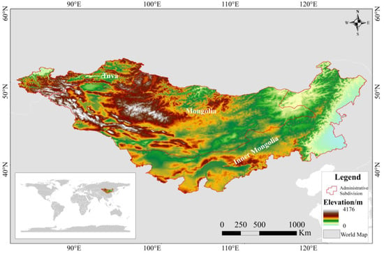
Figure 1.
Study area.
2.2. Data Source and Preprocessing
2.2.1. Remote Sensing Data
The remote sensing data used in this study covers the period from 2000 to 2020, as listed in Table 1. NDVI and EVI data were obtained from the MOD13Q1 dataset provided by Google Earth (https://code.earthengine.google.com/; hereafter referred to as GEE; accessed on 25 October 2022) with a temporal resolution of 16 d. The maximum value synthesis method involves the synthesis of an image by superimposing images from different periods and obtaining the maximum value of the raster cells. Since 2000, the maximum synthesis method has been used to generate the NDVI and EVI data for the MP in summer (June–August). This method can attenuate sudden drops in data caused by atmospheric noise, such as clouds and aerosols [42]. The soil-adjusted vegetation index was obtained from the MOD09A1 dataset provided by the GEE platform band calculations [43] with a temporal resolution of 8 d. Land surface temperature (LST) data with a temporal resolution of eight days were obtained from the MOD11A2 dataset provided by the GEE platform with a temporal resolution of 8 d. The data were processed to generate daily average surface temperature data (unit: °C) for the MP in summer. Precipitation data were obtained from the PERSIANN-CDR dataset provided by the National Oceanic and Atmospheric Administration (https://www.ncei.noaa.gov/; accessed on 6 November 2022) with spatial and temporal resolutions of 0.25° and 1 d, respectively. They were processed to obtain the summed summer precipitation data for the MP. This dataset was extracted by the PERSIANN algorithm using GridSat-B1 infrared satellite data based on a neural network algorithm with high data accuracy and a good application basis in arid areas. All remote sensing data processing in this study was performed using GEE, and all raster data projections were made using the WGS84 projection.

Table 1.
Remote Sensing Data.
2.2.2. Land Cover Data
Land cover data were obtained using GLC_FCS30 (https://data.casearth.cn/sdo/detail/5fbc7904819aec1ea2dd7061; accessed on 19 November 2022), a global 30 m land cover fine classification product published by the Institute of Air and Space Information Innovation of the Chinese Academy of Sciences. The dataset covers the global land area, excluding Antarctica, and contains 29 land cover types, producing land cover products from 1985 to 2020 on a 5-year cycle. Projection transformation, cropping, and resampling tools in ArcGIS were used to generate land cover data for the MP from 2000 to 2020 with a 5-year cycle. The major percentages were as follows: agricultural land, 2.3%; forest, 15.9%; grassland, 46.1%; shrubs, 2.4%; wetland, 0.3%; bare land, 32.4%; and water bodies, 0.7%, with each land cover type remaining essentially constant (<1%) during the study period (2000–2020).
2.2.3. Grass Yield Sample Data
Grass yield sample data were collected by our group during the vegetation-growing seasons (June–August) in 2006, 2013, 2018, 2019, and 2020. The sampling strategy and principle were to select areas with uniform vegetation cover that can represent the condition of the grassland as a sample plot, and in order to ensure a continuous distribution of sample plots within a representative area, the distance between sample plots was approximately 40 km. Due to the inaccessibility of the western part of the Mongolian Plateau, most of the sampling plots are currently concentrated in the northeastern part of the region. We randomly selected three 0.5 m × 0.5 m sample squares within a 50 m × 50 m sample plot with uniform vegetation type. The average of three sample squares was used to represent the herbaceous yield of the sample plot. The sample sites were selected to represent vegetation growth in the region. After data screening and processing, 237 grass yield sample-point data points were obtained. The sampling point coordinate information was imported into ArcGIS10.6 to generate a sampling point vector file, the distribution of which is shown in Figure 2.
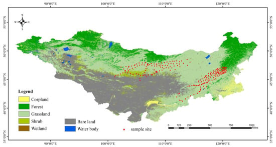
Figure 2.
Mongolian Plateau land cover data.
2.3. Methods
This study comprises the following technical steps: remote sensing image acquisition, training dataset production, model training, prediction, and evaluation. The process is shown in Figure 3. First, images were acquired based on the above data sources, and the images were preprocessed based on GEE to produce the training dataset required for the model. Four models, MLR, RF, KNN, and ANN, were compared, and the best-performing herbaceous yield estimation model was applied to the MP for herbaceous yield estimation.
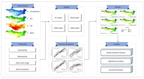
Figure 3.
Grass yield estimation flow chart. EVI: enhanced vegetation index; LST: land surface temperature; NDVI: normalized vegetation index; RF: random forest; MLR: multiple linear regression; KNN: K-nearest neighbor method; ANN: artificial neural network.
2.3.1. Models Parameter Selection
In previous studies, vegetation indices performed better in most cases when fitting models to estimate grass yields [44,45]. In contrast, meteorological factors, such as surface temperature and precipitation, were significantly and positively correlated with actual primary productivity in the MP [25,46]. Therefore, this study selected three variables—vegetation index, land surface temperature, and precipitation—as the input parameters of the four models to estimate grass yield in the MP.
For the initial three models, 70% of the sample point data is allocated for model construction, while the remaining 30% is used for accuracy verification. In contrast, the ANN model is assessed using the K-fold cross-validation method.
2.3.2. Models Construction
MLR Model
The multiple linear regression model minimizes the sum of the squares of the residuals between the predicted and measured values using least squares to determine the optimal parameters [12]. The model was very sensitive to outliers, and the model prediction results were highly susceptible to data outliers. The model can explain the linear relationship between the independent and dependent variables to the maximum extent.
KNN Model
The KNN is a prediction model based on the mean value of the KNN data points [47]. The model does not require significant parameter tuning to achieve a good performance. However, the model has a low generalization ability, is more noise sensitive, and yields good results when dealing with datasets with few features.
RF Model
The RF model is a machine learning model based on the bagging algorithm, which divides the result into different sample datasets by building different decision trees, and the final result is selected by counting the prediction results of each tree using the voting method. Figure 4 illustrates the schematic of the RF model [48]. The model can handle multifeatured datasets without feature selection but produces overfitting on noisy datasets.
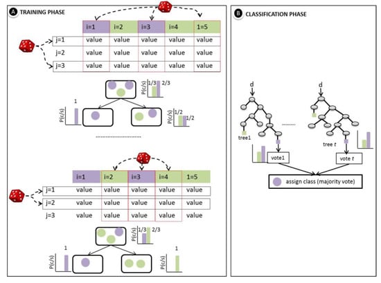
Figure 4.
Schematic of random forest model (cited from [49]).
ANN Model
The deep learning framework used in this study was TensorFlow (GPU version), the model optimizer was selected as RMSprop, and the initial learning rate was set to 0.001. The ANN model schematic is shown in Figure 5 [50]. The number of neurons and hidden layers, the most important parameters in the ANN model, were tested repeatedly and determined to be 18 neurons and 3 hidden layers. The number of neurons from the input to the output layer was as follows (3, 8, 4, 2, 1). The activation functions chosen for each layer of the network were ordinary RELU functions, and the input variables were normalized first. The gradient descent algorithm was selected as the network optimization algorithm. In addition, training would be stopped when the model fit was optimal to avoid overfitting. Because training artificial neural network models requires many samples, this study adopted a k-fold cross-validation (K = 10) approach to solve the problems of insufficient data volume and parameter tuning. In the k-fold cross-validation, we divided the dataset into k copies, used one of them and the remaining k − 1 copies as the validation and training sets, respectively, and then repeated the cross-validation process 10 times, using each k-fold dataset as the validation/test data only once.
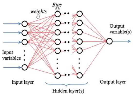
Figure 5.
Schematic of artificial neural network model (cited from [51]).
2.3.3. Accuracy Evaluation
To verify the accuracy of different remote sensing models for herbaceous production estimation, root mean square error (RMSE) and coefficient of determination (R2) are used to measure model accuracy in this paper. The calculation equations are as follows:
where n is the number of measurements, and are the measured and model-predicted values, respectively. In this study, the smaller the RMSE, the higher the accuracy of the model.
where and represent the measured and model-predicted values, respectively, and represents the average of the measured values. R2 is the correlation coefficient between the predicted and measured values, and the closer R2 is to 1, the higher the model accuracy.
2.3.4. Trend Analysis
This study used the Theil–Sen median slope estimation method and Mann–Kendall trend analysis to determine the significance of grass yield trends in the MP over the last 20 years. The evaluation table of grass yield trend was displayed in Table 2. The Theil–Sen median method is a robust nonparametric statistical trend calculation method that fits the trend by taking the median of the slope of any two points in a time series. This method is computationally efficient, independent of extreme values, suitable for long-time series analysis, and is widely used in meteorology and seasonal environmental data analysis [52]. The formula is as follows:
where β is the slope between two points in the time series; and are the data values corresponding to time points j and k (j > k) in the time series, respectively.

Table 2.
Evaluation table of the grass yield trend (β is Theil–Sen median slope, Z is normalized test statistic).
The Mann–Kendall trend analysis method is a nonparametric time-series trend test with the advantage that it does not require data to obey a normal distribution and is not affected by missing data and extreme values [53]. For time-series data = ,…, , the test statistic S is calculated as follows:
When n > 10, the variance of its test statistic S is:
where n represents the number of data points in the series, and and are the data values corresponding to time points i and j (j > i) in the time series, respectively.
3. Results
3.1. Multi-Factor Models Comparison
For accuracy, the four herbaceous yield estimation models used were the ANN, RF, KNN, and MLR. It is shown in Figure 6. The accuracy of the ANN model (R2 = 0.78, RMSE = 48.7 g/m2) and RF model (R2 = 0.72, RMSE = 55.28 g/m2) was significantly higher than that of the other two models, and both of them could be used in grass yield estimation in the MP. While the KNN model accuracy followed, the MLR model could only characterize 40% of the variance. Therefore, we used the ANN model to estimate the grass yield in the MP between 2000 and 2020.
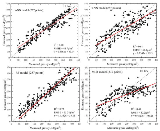
Figure 6.
Accuracy evaluation of different grass yield simulated methods. RF: random forest; RMSE: root mean square error.
3.2. Single-factor Model Comparison
The purpose of building univariate models is to select the most effective vegetation index for grass production inversion (the process of obtaining ground-based grass yield from remote sensing data) and to optimize the models’ performance. The number of sample points used for all models was 237. It is shown in Table 3. A significant positive correlation was observed between grass yield and the vegetation indexes in the MP, indicating the feasibility of using a single vegetation index to monitor grass yield in the region. However, the established relationship between grass yield and vegetation indices can also greatly impact the model’s estimation accuracy. The fitting accuracy of one of the linear regression models was significantly lower than that of the other three types of nonlinear models. Nevertheless, the linear regression model reflected the correlation between the vegetation index and grass yield more intuitively. Similarly, different vegetation indices reflected different effects on grass production in different regions. NDVI had the highest correlation coefficient with grass yield, indicating that NDVI could better reflect changes in grass yield than the other indices in the MP. The results show that the NDVI power function model is a simple and effective method for monitoring grass yields. Although the performance of the ANN model is better than that of the conventional model, the selected variables and the model constructed in this study are applicable only to the MP.

Table 3.
Fitting models among vegetation index and grass yield.
3.3. Spatial and Temporal Variability of Overall Grass Production in the MP
We masked the forested areas because of errors in the estimation of grass yield in the forested areas caused by the cover of the forest canopy over ground grass (Figure 7). Clear spatial heterogeneity was observed in grass yield in the MP, and the distribution of grass yield gradually increased from south to north (Figure A1). The high grass-production areas are mainly located in the southern part of Inner Mongolia and the Selengar River Basin in Mongolia, two areas with flat terrain, sufficient annual precipitation, dense small rivers throughout the region, rich in hydro-energy resources, and a natural environment suitable for grass growth. In contrast, the low-grass production area is concentrated in southwestern Mongolia, which is affected by an arid climate, low vegetation cover, short growing seasons, mostly bare land and shrubs, and easy soil moisture loss, resulting in the lowest grass productivity. Most grasslands in the MP produced 250–350 g/m2 of grass.
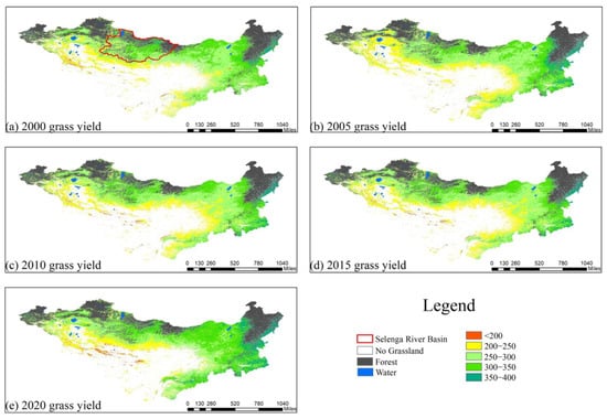
Figure 7.
Spatial and temporal distribution of grass yield in the Mongolian Plateau in 2000, 2010, and 2020.
Overall, grassland productivity in the MP has increased. It is shown in Figure 8. From 2000 to 2020, the average annual grass yield in the MP varied between 270.1 and 304.3 g/m2, with the lowest value of 270.1 g/m2 reached in the study area in 2001 and the peak of 304.3 g/m2 in 2018. The fitted curve shows that the average annual grass production in the MP increased at a rate of 1 g/m2 per year, indicating that the grassland ecology of the MP gradually recovered. Earlier research found that grassland productivity gradually increased at high latitudes and altitudes in the Northern Hemisphere due to global warming and the greenhouse effect, validating our findings [54]. However, in 2001, 2007, and 2009, there was a significant decrease in the average annual grass production, which was found to be due to a major disaster in the MP, resulting in a sudden decrease in grass yield. In 2001, a major snowstorm in the MP caused Mongolia to lose nearly 10% of its gross domestic product and caused severe damage to its agriculture and livestock industries. In 2007 and 2009, spring precipitation in the northeastern region of the Mongolian Plateau was 50–80% lower than that in the same period. The temperature reached a maximum for the same period, and high temperatures and low rainfall directly led to a sudden decrease in grassland productivity. In general, the ecological structure of the MP is simple and vulnerable to extreme climatic conditions. However, the overall ecological environment is improving annually.
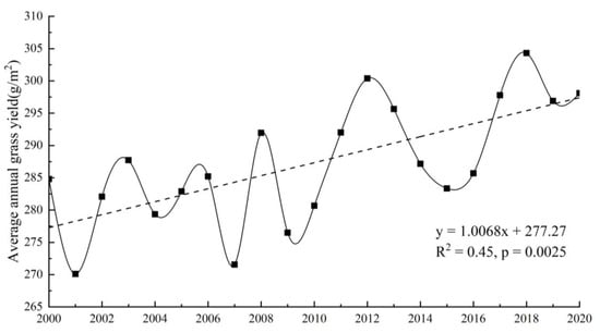
Figure 8.
Changes in average annual grass yield in the Mongolian Plateau.
3.4. Trend Analysis of Grass Yield
Over 90% of the MP showed an increasing trend in grass production from 2000 to 2020, with nearly 40% of the areas showing a significant increase. It is shown in Figure 9. These areas are primarily located in northern and southeastern Inner Mongolia. Approximately 10% of the areas showed a decreasing trend in grass production, mainly in western Mongolia, the central Tuva Republic, and central Inner Mongolia; 1.43% of the significantly decreasing areas were concentrated in Inner and central Mongolia near the Gobi Steppe.
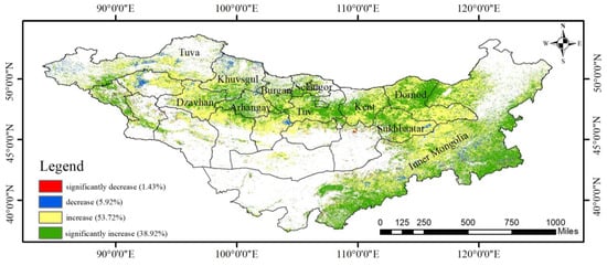
Figure 9.
Trends in grass yield in the Mongolian Plateau from 2000 to 2020.
It is shown in Table 4. By region, the three provinces of Mongolia—Kent, Dornod, and Tuv—showed an increasing trend in 99% grassland productivity. In contrast, grassland productivity in the Tuv Province significantly increased by more than 90%. Tuva Republic, Khuvsgul Province, and Inner Mongolia had the largest shares of declining grass production areas. Although the area of grassland decline in the Tuva Republic and Khuvsgul Province was extensive (approximately 15%), its significant decline was less than 1%, which is far less than the 1.44% significant decline in grassland production in Inner Mongolia.

Table 4.
Trends in grass yield in various regions of the Mongolian Plateau.
4. Discussion
4.1. Model Variables Analysis
4.1.1. Sensitivity Analysis of Model Variables
Because deep learning models are usually considered black box models, and it is impossible to estimate the importance of each feature for model prediction, we analyzed the model using the mean impact value method in the sensitivity analysis method based on the perturbation of the input variables. The mean impact value method increases each variable feature by 10% on the training sample into a simulation sample after the network training is terminated. The difference between the fitted result of the simulation sample and the original prediction is considered as the value of the change in the effect of the variable on the output, thus determining the importance of the effect of the respective variable on the model output.
The results are shown in Figure 10. Overall, the average percentage changes in the output resulting from the increased perturbations of the three variables (NDVI, LST, precipitation) were 4.04%, 2.34%, and 2.09%. The greatest mean perturbation change of 4.04% was observed for NDVI and the lowest mean perturbation change of 2.09% was observed for precipitation. The results show that the importance of the three variables to the model output, in descending order, was NDVI, LST, and precipitation. By analyzing each variable independently, both the NDVI and LST variables remained highly sensitive to the output results in the high-value region, whereas the low-value region also increased with perturbation. Areas with high NDVI were concentrated in northeastern Inner Mongolia.
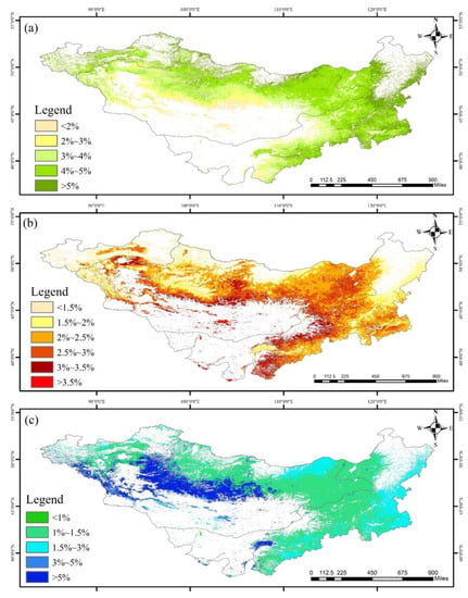
Figure 10.
Sensitivity analysis of model variables, which are listed as follows: (a) sensitivity analysis of the model to NDVI; (b) sensitivity analysis of the model to LST; (c) sensitivity analysis of the model to precipitation. NDVI: normalized vegetation index; LST: land surface temperature.
In contrast, areas with high LST were concentrated in central Inner Mongolia. These areas had the highest percentage of added value as NDVI and LST perturbations increased. This indicates that grass production is more sensitive to the two variables, NDVI and LST, or that the two variables are significantly and positively correlated with grass productivity in the MP. Regarding precipitation, the perturbation variation was smaller in regions with abundant precipitation in the northern part of the MP. The perturbation variation was larger in water-scarce regions in central and western Mongolia. This indicates that the sensitivity to precipitation is low in some areas of the MP, and precipitation is not significantly and positively correlated with grass yield.
4.1.2. Permutation Feature Importance
Permutation feature importance (PFI) is an algorithm that can directly calculate the importance of input features. To assess the importance of features, this method confuses the data arrangement of a specific feature while keeping the remaining features unchanged. Subsequently, it calculates the difference (the result of subtraction) between the prediction results before and after the confusion to evaluate the feature’s importance. The three features (NDVI, LST, precipitation) were randomly confused ten times, and the average of the results was calculated. Figure 11 shows the result of LST being randomly confused once. The feature importance, from the highest to the lowest, was LST at 0.042, NDVI at 0.028, and precipitation at 0.014. Consequently, our findings indicate that LST exhibits greater importance in the ANN model compared with NDVI and precipitation. LST emerges as a significant factor that strongly influences the prediction results of the model. The MIV method reversed the importance of NDVI and LST, and the phenomenon could potentially be attributed to its heightened sensitivity to data noise, which impacted the interpretability of the model.
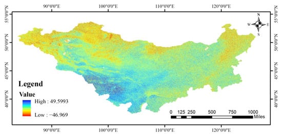
Figure 11.
Permutation feature importance result of land surface temperature (one time).
4.2. Comparison with Other Studies
This study used an ANN model to quantify grass production in the MP over the last 20 years with an accuracy comparable to that of net primary productivity (NPP) or aboveground biomass (AGB)-related studies. Bao et al. estimated the average NPP of 228.2 gC/m2 based on the CASA model for the growing season in Mongolia during 1982–2011 and found that the sensitivity of vegetation growth to precipitation decreased in areas with sufficient precipitation in northern Mongolia, which is consistent with our study [55]. John et al. used a regression tree model to estimate AGB in the MP, and the validation results showed that its R2 and RMSE were 0.73 and 76.9 g/m2, respectively [51]. Similarly, the poor sensitivity of grass growth to temperature in the Inner Mongolia region supports previous studies in the Inner Mongolia region (Su et al.) [39]. In line with our prior experimental findings indicating a rising trend in grassland productivity, the study conducted by Yan et al. examined the carrying capacity of Mongolian grasslands over the period from 2000 to 2020. Their research corroborated our results, revealing that approximately 98.5% of the Mongolian area exhibited a significant increase in AGB [56].
In addition, we analyzed the reasons for the performance of the four models. The RF model may overfit noisy sample points during the training process, resulting in a lower accuracy rate than that of the ANN model. In contrast, the KNN model can hardly learn the meteorology factor characteristics from the data, and the MLR cannot fit the nonlinear relationship between grass production and variables, resulting in a lower accuracy than the ANN and RF models, which have better learning ability. A study in Xilingole, Inner Mongolia, of grassland AGB compared an ANN model (R2 = 0.81, RMSE = 60) to an MLR model (R2 = 0.59, RMSE = 74). It was considered that the ANN model was more applicable than that of the MLR model to observing biomass [33]. In a separate study focusing on AGB estimation, Gao et al. evaluated multiple modeling approaches, including RF (RMSE = 26.8), KNN (RMSE = 28), ANN (RMSE = 25.5), LR (RMSE = 27.4), and support vector regression (SVR) (RMSE = 25.8) [57]. The authors found that among these approaches, the ANN model exhibited superior performance and was identified as the most effective method for enhancing AGB estimation.
4.3. Model Advantages and Limitations
The ANN model possesses the capability to autonomously select model input data and learn input features, rendering it highly adaptable and versatile. Moreover, by adjusting hyperparameters and network structure, the ANN model can construct the most suitable models tailored to different regions and features. This flexibility enhances its applicability and effectiveness across various scenarios. Simultaneously, the model prediction accuracy can be continuously improved by increasing the number of training samples. However, this model has certain limitations. First, the learning process of the ANN model is not controllable. Although we performed a variable sensitivity analysis on the model to obtain a general idea of the effect of the model inputs on the prediction results, the sum of the perturbation changes in the three variables was not equal to the perturbation itself, indicating that nonlinear input perturbation effects among them were not observable. Second, the learning process of the model demands a greater number of training samples, and in the less-sampled regions, particularly in the western part of the MP, the error tends to be larger.
5. Conclusions
Faced with the challenges of long-term grassland yield monitoring in the MP, we compared four different models based on three variables (NDVI, LST, precipitation) to estimate grass yield and quantitatively assessed changes in grass productivity from 2000 to 2020 based on the optimal model. The following conclusions were obtained: (1) The estimation accuracy of the ANN model was higher than that of the KNN, MLR, RF, and vegetation index single-factor models (R2 = 0.78, RMSE = 48.7 g/m2). (2) Grassland productivity in the MP showed significant spatial heterogeneity and decreased from northeast to southwest. During the study period, grassland productivity increased in 90% of the Mongolian Plateau. (3) The overall climate of the Mongolian Plateau was warm and humid, and grass production was positively correlated with NDVI, LST, and precipitation. However, the sensitivity of grass production to the NDVI and LST was high. LST was the most important factor affecting grassland growth in the MP. This study also has limitations for not well-distributed samples. With more samples collected in the full coverage of the MP, this estimation results accuracy can be increased in the near future.
Author Contributions
M.L. and J.W. designed the study, processed the data, and drafted the manuscript. K.L. helped to design the study, provided knowledge and experience in technology, and reviewed the manuscript. A.O., C.T., and C.X. provided advice on the study and reviewed the manuscript. All authors have read and agreed to the published version of the manuscript.
Funding
This research was funded by the National Key R&D Program of China (2022YFE0119200), Project “32161143025” supported by NSFC, Science & Technology Fundamental Resources Investigation Program of China (2022FY101902), Mongolian Foundation for Science and Technology (NSFC_2022/01, CHN2022/276), National University of Mongolia (P2023-4429), Key Project of Innovation LREIS (KPI006), and Construction Project of China Knowledge Center for Engineering Sciences and Technology (CKCEST-2022-1-41).
Data Availability Statement
Not applicable.
Acknowledgments
The authors are grateful for the support provided by the National University of Mongolia.
Conflicts of Interest
The authors declare no conflict of interest.
Appendix A
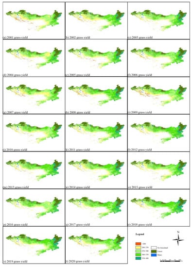
Figure A1.
Annual grass production in the Mongolian Plateau from 2001 to 2020.
References
- Liu, H.; Zhang, A.; Zhao, Y.; Zhao, A.; Wang, D. Spatial scale transformation–based estimation model for fresh grass yield: A case study of the Xilingol Grassland, Inner Mongolia, China. Environ. Sci. Pollut. Res. 2022, 30, 1085–1095. [Google Scholar] [CrossRef] [PubMed]
- Zhao, F.; Xu, B.; Yang, X.; Jin, Y.; Li, J.; Xia, L.; Chen, S.; Ma, H. Remote Sensing Estimates of Grassland Aboveground Biomass Based on MODIS Net Primary Productivity (NPP): A Case Study in the Xilingol Grassland of Northern China. Remote Sens. 2014, 6, 5368–5386. [Google Scholar] [CrossRef]
- Li, Q.; Wang, J.; Xie, H.; Ochir, A.; Davaasuren, D. Applicability of Grassland Production Estimation Using Remote Sensing for the Mongolian Plateau by Comparing Typical Regions in China and Mongolia. Sustainability 2022, 14, 3122. [Google Scholar] [CrossRef]
- Wei, Y.; Zhen, L. The dynamics of livestock and its influencing factors on the Mongolian Plateau. Environ. Dev. 2020, 34, 100518. [Google Scholar] [CrossRef]
- Qin, P.; Sun, B.; Li, Z.; Gao, Z.; Li, Y.; Yan, Z.; Gao, T. Estimation of Grassland Carrying Capacity by Applying High Spatiotemporal Remote Sensing Techniques in Zhenglan Banner, Inner Mongolia, China. Sustainability 2021, 13, 3123. [Google Scholar] [CrossRef]
- Ali, I.; Cawkwell, F.; Green, S.; Dwyer, N. Application of statistical and machine learning models for grassland yield estimation based on a hypertemporal satellite remote sensing time series. In Proceedings of the 2014 IEEE Geoscience and Remote Sensing Symposium, Quebec City, QC, Canada, 13–18 July 2014; pp. 5060–5063. [Google Scholar] [CrossRef]
- Wang, L.; Yu, H.Y.; Zhang, Q.; Xu, Y.; Tao, Z.; Alatalo, J.; Dai, J. Responses of aboveground biomass of alpine grass-lands to climate changes on the Qinghai-Tibet Plateau. J. Geogr. Sci. 2018, 28, 1953–1964. [Google Scholar]
- Dusseux, P.; Guyet, T.; Pattier, P.; Barbier, V.; Nicolas, H. Monitoring of grassland productivity using Sentinel-2 remote sensing data. Int. J. Appl. Earth Obs. Geoinf. 2022, 111, 102843. [Google Scholar] [CrossRef]
- Song, X.; Mi, N.; Mi, W.; Li, L. Spatial non-stationary characteristics between grass yield and its influencing factors in the Ningxia temperate grasslands based on a mixed geographically weighted regression model. J. Geogr. Sci. 2022, 32, 1076–1102. [Google Scholar] [CrossRef]
- Motlagh, M.G.; Kafaky, S.B.; Mataji, A.; Akhavan, R. Estimating and mapping forest biomass using regression models and Spot-6 images (case study: Hyrcanian forests of north of Iran). Environ. Monit. Assess. 2018, 190, 352. [Google Scholar] [CrossRef]
- Xue, J.; Ge, Y.; Ren, H. Spatial upscaling of green aboveground biomass derived from MODIS-based NDVI in arid and semiarid grasslands. Adv. Space Res. 2017, 60, 2001–2008. [Google Scholar] [CrossRef]
- You, H.; Luo, C.; Liu, Z.; Wang, J. Study on the Method of Grass Yield Model in the Source Region of Three Rivers with Multivariate Data. IOP Conf. Ser. Earth Environ. Sci. 2014, 17, 012031. [Google Scholar] [CrossRef]
- Zhang, Y.; Wang, R. RETRACTED: Estimation of aboveground biomass of vegetation based on landsat 8 OLI images. Heliyon 2022, 8, e11099. [Google Scholar] [CrossRef] [PubMed]
- Yang, X.C.; Xu, B.; Jin, Y.X.; Li, J.Y.; Zhu, X.H. On Grass Yield Remote Sensing Estimation Models of China’s Northern Farming-Pastoral Ecotone. In Advances in Computational Environment Science; Springer: Berlin/Heidelberg, Germany, 2012; Volume 142, pp. 281–291. [Google Scholar] [CrossRef]
- Liu, J.; Atzberger, C.; Huang, X.; Shen, K.; Liu, Y.; Wang, L. Modeling grass yields in Qinghai Province, China, based on MODIS NDVI data—An empirical comparison. Front. Earth Sci. 2020, 14, 413–429. [Google Scholar] [CrossRef]
- Ali, A.; Lin, S.; He, J.; Kong, F.; Yu, J.; Jiang, H. Elucidating space, climate, edaphic, and biodiversity effects on aboveground biomass in tropical forests. Land Degrad. Dev. 2019, 30, 918–927. [Google Scholar] [CrossRef]
- Timothy, D.; Onisimo, M.; Cletah, S.; Adelabu, S.; Tsitsi, B. Remote sensing of aboveground forest biomass: A review. Trop. Ecol. 2016, 57, 125–132. [Google Scholar]
- Wu, C.; Chen, K.; E, C.; You, X.; He, D.; Hu, L.; Liu, B.; Wang, R.; Shi, Y.; Li, C.; et al. Improved CASA model based on satellite remote sensing data: Simulating net primary productivity of Qinghai Lake basin alpine grassland. Geosci. Model Dev. 2022, 15, 6919–6933. [Google Scholar] [CrossRef]
- Yu, D.; Shi, P.; Shao, H.; Zhu, W.; Pan, Y. Modelling net primary productivity of terrestrial ecosystems in East Asia based on an improved CASA ecosystem model. Int. J. Remote Sens. 2009, 30, 4851–4866. [Google Scholar] [CrossRef]
- Goetz, S.J.; Prince, S.D.; Small, J.; Gleason, A.C.R. Interannual variability of global terrestrial primary production: Results of a model driven with satellite observations. J. Geophys. Res. Atmos. 2000, 105, 20077–20091. [Google Scholar] [CrossRef]
- Hadian, F.; Jafari, R.; Bashari, H.; Tartesh, M.; Clarke, K.D. Estimation of spatial and temporal changes in net primary production based on Carnegie Ames Stanford Approach (CASA) model in semi-arid rangelands of Semirom County, Iran. J. Arid Land 2019, 11, 477–494. [Google Scholar] [CrossRef]
- Nayak, R.K.; Patel, N.R.; Dadhwal, V.K. Estimation and analysis of terrestrial net primary productivity over India by remote-sensing-driven terrestrial biosphere model. Environ. Monit. Assess. 2009, 170, 195–213. [Google Scholar] [CrossRef]
- Zhang, J.; Zhang, L.; Liu, X.; Qiao, Q. Research on Sustainable Development in an Alpine Pastoral Area Based on Equilibrium Analysis Between the Grassland Yield, Livestock Carrying Capacity, and Animal Husbandry Population. Sustainability 2019, 11, 4659. [Google Scholar] [CrossRef]
- Bao, G.; Bao, Y.; Qin, Z.; Xin, X.; Bao, Y.; Bayarsaikan, S.; Zhou, Y.; Chuntai, B. Modeling net primary productivity of terrestrial ecosystems in the semi-arid climate of the Mongolian Plateau using LSWI-based CASA ecosystem model. Int. J. Appl. Earth Obs. Geoinf. 2016, 46, 84–93. [Google Scholar] [CrossRef]
- Tang, R.; Zhao, Y.; Lin, H. Spatio-Temporal Variation Characteristics of Aboveground Biomass in the Headwater of the Yellow River Based on Machine Learning. Remote Sens. 2021, 13, 3404. [Google Scholar] [CrossRef]
- Liang, T.; Feng, Q.; Ge, J.; Xie, H.; Liang, T. Assessment of Machine Learning Methods for Modeling Alpine Grassland Biomass in Southern Qinghai Province, China. In Proceedings of the 3rd International Conference on Computer Science and Application Engineering, Sanya, China, 22–24 October 2019; 77. [Google Scholar] [CrossRef]
- Opelele, O.; Yu, Y.; Fan, W.; Chen, C.; Kachaka, S. Biomass Estimation Based on Multilinear Regression and Machine Learning Algorithms in the Mayombe Tropical Forest, in the Democratic Republic of Congo. Appl. Ecol. Environ. Res. 2021, 19, 359–377. [Google Scholar] [CrossRef]
- Qiu, A.; Yang, Y.; Wang, D.; Xu, S.; Wang, X. Exploring parameter selection for carbon monitoring based on Landsat-8 imagery of the aboveground forest biomass on Mount Tai. Eur. J. Remote Sens. 2019, 53, 4–15. [Google Scholar] [CrossRef]
- Tang, Z.; Xia, X.; Huang, Y.; Lu, Y.; Guo, Z. Estimation of National Forest Aboveground Biomass from Multi-Source Remotely Sensed Dataset with Machine Learning Algorithms in China. Remote Sens. 2022, 14, 5487. [Google Scholar] [CrossRef]
- Liu, W.; Xu, C.; Zhang, Z.; De Boeck, H.; Wang, Y.; Zhang, L.; Xu, X.; Zhang, C.; Chen, G.; Xu, C. Machine learning-based grassland aboveground biomass estimation and its response to climate variation in Southwest China. Front. Ecol. Evol. 2023, 11, 1146850. [Google Scholar] [CrossRef]
- Haywood, A.; Stone, C.; Jones, S. The potential of sentinel satellites for large area aboveground forest biomass mapping. In Proceedings of the IEEE International Geoscience and Remote Sensing Symposium, Valencia, Spain, 22–27 July 2018. [Google Scholar]
- Tian, Y.; Huang, H.; Zhou, G.; Zhang, Q.; Tao, J.; Zhang, Y.; Lin, J. Aboveground mangrove biomass estimation in Beibu Gulf using machine learning and UAV remote sensing. Sci. Total Environ. 2021, 781, 146816. [Google Scholar] [CrossRef]
- Xie, Y.; Sha, Z.; Yu, M.; Bai, Y.; Zhang, L. A comparison of two models with Landsat data for estimating above ground grassland biomass in Inner Mongolia, China. Ecol. Model. 2009, 220, 1810–1818. [Google Scholar] [CrossRef]
- Yang, S.; Feng, Q.; Liang, T.; Liu, B.; Zhang, W.; Xie, H. Modeling grassland above-ground biomass based on artificial neural network and remote sensing in the Three-River Headwaters Region. Remote Sens. Environ. 2018, 204, 448–455. [Google Scholar] [CrossRef]
- Gao, Q.; Zhu, W.; Schwartz, M.W.; Ganjurjav, H.; Wan, Y.; Qin, X.; Ma, X.; Williamson, M.A.; Li, Y. Climatic change controls productivity variation in global grasslands. Sci. Rep. 2016, 6, 26958. [Google Scholar] [CrossRef] [PubMed]
- Lei, T.; Wu, J.; Wang, J.; Shao, C.; Wang, W.; Chen, D.; Li, X. The Net Influence of Drought on Grassland Productivity over the Past 50 Years. Sustainability 2022, 14, 12374. [Google Scholar] [CrossRef]
- Li, G.; Yu, L.; Liu, T.; Bao, Y.; Yu, J.; Xin, B.; Bao, L.; Li, X.; Chang, X.; Zhang, S. Spatial and temporal variations of grassland vegetation on the Mongolian Plateau and its response to climate change. Front. Ecol. Evol. 2023, 11, 1067209. [Google Scholar] [CrossRef]
- Shao, J.; Zhou, X.; Groenigen, K.J.; Zhou, G.; Zhou, H.; Zhou, L.; Lu, M.; Xia, J.; Jiang, L.; Hungate, B.A.; et al. Warming effects on grassland productivity depend on plant diversity. Glob. Ecol. Biogeogr. 2021, 31, 588–598. [Google Scholar] [CrossRef]
- Su, R.; Yu, T.; Dayananda, B.; Bu, R.; Su, J.; Fan, Q. Impact of climate change on primary production of Inner Mongolian grasslands. Glob. Ecol. Conserv. 2020, 22, e00928. [Google Scholar] [CrossRef]
- John, R.; Chen, J.; Giannico, V.; Park, H.; Xiao, J.; Shirkey, G.; Ouyang, Z.; Shao, C.; Lafortezza, R.; Qi, J. Grassland canopy cover and aboveground biomass in Mongolia and Inner Mongolia: Spatiotemporal estimates and controlling factors. Remote Sens. Environ. 2018, 213, 34–48. [Google Scholar] [CrossRef]
- Narisu, N.; Bao, Y.; Bao, Y. Drought Temporal Variation Characteristics Analysis based on the PDSI Data in Mongolian Plateau. In Proceedings of the 7th Annual Meeting of Risk Analysis Council of China Association for Disaster Prevention (RAC-2016), Changsha, China, 4–6 November 2016; pp. 843–848. [Google Scholar]
- Baghi, N.G.; Oldeland, J. Do soil-adjusted or standard vegetation indices better predict above ground biomass of semi-arid, saline rangelands in North-East Iran? Int. J. Remote Sens. 2019, 40, 8223–8235. [Google Scholar] [CrossRef]
- Nakano, T.; Bavuudorj, G.; Urianhai, N.G.; Shinoda, M. Monitoring aboveground biomass in semiarid grasslands using MODIS images. J. Agric. Meteorol. 2013, 69, 33–39. [Google Scholar] [CrossRef]
- Gang, B.; Hasituya; Hugejiletu; Bao, Y. Remotely sensed estimate of biomass carbon stocks in Xilingol grassland using MODIS NDVI data. In Proceedings of the International Conference on Mechatronic Sciences, Electric Engineering and Computer (MEC), Shenyang, China, 20–22 December 2013; pp. 676–679. [Google Scholar]
- Wehlage, D.C. Monitoring Year-to-Year Variability in Dry Mixed-Grass Prairie Yield Using Multi-Sensor Remote Sensing. Master’s Thesis, University of Alberta, Edmonton, AB, Canada, 2012. [Google Scholar]
- Yin, C.; Luo, M.; Meng, F.; Sa, C.; Yuan, Z.; Bao, Y. Contributions of Climatic and Anthropogenic Drivers to Net Primary Productivity of Vegetation in the Mongolian Plateau. Remote Sens. 2022, 14, 3383. [Google Scholar] [CrossRef]
- Hong, Y.S.; Heo, J.; Jung, J.; Han, S.H.; Kim, K.M. Estimation of Aboveground Biomass Carbon Stock Using Landsat TM and Ratio Images—kNN algorithm and Regression Model Priority. J. Korean Soc. Geospat. Inf. Sci. 2011, 19, 39–48. [Google Scholar]
- Xia, J.; Ma, M.; Liang, T.; Wu, C.; Yang, Y.; Zhang, L.; Zhang, Y.; Yuan, W. Estimates of grassland biomass and turnover time on the Tibetan Plateau. Environ. Res. Lett. 2017, 13, 014020. [Google Scholar] [CrossRef]
- Belgiu, M.; Drăguţ, L. Random forest in remote sensing: A review of applications and future directions. ISPRS J. Photogramm. Remote Sens. 2016, 114, 24–31. [Google Scholar] [CrossRef]
- Wang, L.; Liu, J.; Xu, S.; Dong, J.; Yang, Y. Forest Above Ground Biomass Estimation from Remotely Sensed Imagery in the Mount Tai Area Using the RBF ANN Algorithm. Intell. Autom. Soft Comput. 2018, 24, 391–398. [Google Scholar] [CrossRef]
- Kisi, O.; Alizamir, M.; Zounemat-Kermani, M. Modeling groundwater fluctuations by three different evolutionary neural network techniques using hydroclimatic data. Nat. Hazards 2017, 87, 367–381. [Google Scholar] [CrossRef]
- Bolton, D.K.; Tompalski, P.; Coops, N.C.; White, J.C.; Wulder, M.A.; Hermosilla, T.; Queinnec, M.; Luther, J.E.; van Lier, O.R.; Fournier, R.A.; et al. Optimizing Landsat time series length for regional mapping of lidar-derived forest structure. Remote Sens. Environ. 2020, 239, 111645. [Google Scholar] [CrossRef]
- Prăvălie, R.; Niculiţă, M.; Roşca, B.; Patriche, C.; Dumitraşcu, M.; Marin, G.; Nita, I.-A.; Bandoc, G.; Birsan, M.-V. Modelling forest biomass dynamics in relation to climate change in Romania using complex data and machine learning algorithms. Stoch. Environ. Res. Risk Assess. 2023, 37, 1669–1695. [Google Scholar] [CrossRef]
- Yuan, M.; Zhu, Q.; Zhang, J.; Liu, J.; Chen, H.; Peng, C.; Li, P.; Li, M.; Wang, M.; Zhao, P. Global response of terrestrial gross primary productivity to climate extremes. Sci. Total Environ. 2020, 750, 142337. [Google Scholar] [CrossRef]
- Bao, G.; Tuya, A.; Bayarsaikhan, S.; Dorjsuren, A.; Mandakh, U.; Bao, Y.; Li, C.; Vanchindorj, B. Variations and climate constraints of terrestrial net primary productivity over Mongolia. Quat. Int. 2019, 537, 112–125. [Google Scholar] [CrossRef]
- Yan, N.; Zhu, W.; Wu, B.; Tuvdendorj, B.; Chang, S.; Mishigdorj, O.; Zhang, X. Assessment of the grassland carrying capacity for winter-spring period in Mongolia. Ecol. Indic. 2023, 146, 109868. [Google Scholar] [CrossRef]
- Gao, Y.; Lu, D.; Li, G.; Wang, G.; Chen, Q.; Liu, L.; Li, D. Comparative Analysis of Modeling Algorithms for Forest Aboveground Biomass Estimation in a Subtropical Region. Remote Sens. 2018, 10, 627. [Google Scholar] [CrossRef]
Disclaimer/Publisher’s Note: The statements, opinions and data contained in all publications are solely those of the individual author(s) and contributor(s) and not of MDPI and/or the editor(s). MDPI and/or the editor(s) disclaim responsibility for any injury to people or property resulting from any ideas, methods, instructions or products referred to in the content. |
© 2023 by the authors. Licensee MDPI, Basel, Switzerland. This article is an open access article distributed under the terms and conditions of the Creative Commons Attribution (CC BY) license (https://creativecommons.org/licenses/by/4.0/).