Remote Sensing Neural Radiance Fields for Multi-View Satellite Photogrammetry

Abstract

Neural radiance fields (NeRFs) combining machine learning with differentiable rendering have arisen as one of the most promising approaches for novel view synthesis and depth estimates. However, NeRFs only applies to close-range static imagery and it takes several hours to train the model. The satellites are hundreds of kilometers from the earth. Satellite multi-view images are usually captured over several years, and the scene of images is dynamic in the wild. Therefore, multi-view satellite photogrammetry is far beyond the capabilities of NeRFs. In this paper, we present a new method for multi-view satellite photogrammetry of Earth observation called remote sensing neural radiance fields (RS-NeRFs). It aims to generate novel view images and accurate elevation predictions quickly. For each scene, we train an RS-NeRF using high-resolution optical images without labels or geometric priors and apply image reconstruction losses for self-supervised learning. Multi-date images exhibit significant changes in appearance, mainly due to cars and varying shadows, which brings challenges to satellite photogrammetry. Robustness to these changes is achieved by the input of solar ray direction and the vehicle removal method. NeRFs make it intolerable by requiring a very long time to train an easy scene. In order to significantly reduce the training time of RS-NeRFs, we build a tiny network with HashEncoder and adopted a new sampling technique with our custom CUDA kernels. Compared with previous work, our method performs better on novel view synthesis and elevation estimates, taking several minutes.

1. Introduction

High-resolution satellite images are a valuable resource in many economic activities, and many activities are based on understanding the geometric shape and its changes on the Earth’s surface. Although many people believe satellite images are taken from a vertical angle, they are almost always taken from an oblique angle. These non-vertical satellite images provide information about vertical structures and can also be used to estimate 3D shapes. In addition, the combination of images from different viewpoints can reveal aspects that cannot be captured using a single image. One of the goals of multi-view image tasks (such as SPOT6-7 [1] and WorldView-3 [2]) is to estimate the terrain of the Earth’s land cover. This knowledge is relevant to many applications in remote sensing, including terrain mapping for flood risk mitigation [3], biomass estimation [4], land cover classification [5], and change detection [6].

Although active sensors such as LiDAR can directly measure the distance from a satellite to the ground, they require a significant amount of energy compared to passive cameras. Therefore, many pipelines have been developed to accurately estimate depth from disparity using multiple satellite views [7,8,9,10,11,12,13]. The resulting large-scale 3D models are typically represented using either a discrete point cloud or a digital surface model (DSM). However, these models rely on manually designed matching strategies and cost functions and lack consensus when merging output results from different pairs [14].

Satellite measurements mainly focus on geometric accuracy, while novel view synthesis aims to obtain realistic image models. Novel view synthesis is a continuously developing technology that uses a set of input images and their camera poses of a given scene to render the observed scene content from previously unobserved viewpoints, allowing users to navigate the reconstructed environment with high visual fidelity. Recently, neural rendering techniques such as neural radiance fields (NeRFs) [15] have enabled realistic reconstruction and novel view synthesis given a set of camera positions and images [16,17,18]. Early research was often focused on small-scale and object-centric reconstruction, while some methods have begun considering scenes the size of a single room or building, these methods are often limited and cannot be directly applied to urban-scale environments. Using these methods in large-scale environments often leads to significant artifacts and low visual fidelity due to limited model capacity.

Reconstructing large-scale environments can serve various vital purposes, such as autonomous driving [19,20,21] and aerial surveying [22,23]. For example, it can be used for mapping and creating high-fidelity maps of the entire operational domain as a powerful prior for various problems, including robot localization, navigation, and collision avoidance. Large-scale scene reconstruction can also be used for closed-loop robot simulation [24]. For instance, Block-NeRFs [25] used 2.8 million images to perform street view reconstruction of the San Francisco Alamo Square community.

Our study employs an improved NeRF model that relies only on 10-20 high-resolution satellite images to achieve elevation estimation and novel view synthesis of urban and suburban areas in minutes. These applications could include using micro/nano satellites for Earth observation with limited available energy or for exploring other planets [3], comets, or asteroids. This technology could also help people in war-torn areas reconstruct their former homes in the future.

While neural radiance fields (NeRFs) have shown impressive performance in novel view synthesis tasks, there are several limitations that prevent their direct application to multi-view satellite photogrammetry and novel view synthesis. Classic NeRF reconstruction and rendering are performed on data that is generated in strictly controlled lab conditions or using software such as Blender. A NeRF assumes a constant density, radiance, and illumination of the target 3D scene, with a focus primarily on object-centric reconstruction at a small scale. However, when using NeRFs to reconstruct large-scale environments captured by satellites, additional challenges arise, such as limited model capacity, the introduction of dynamic scenes (such as cars and shadow regions), and excessively long training times. Even for simple Lego reconstructions, NeRF training can take several hours, necessitating shortening training times. Furthermore, since NeRFs are designed for close-range images, its sampling methods cannot be directly applied to satellite photogrammetry, especially in the case of remote-sensing satellites hundreds of kilometers away from the Earth.

To address these limitations, we improved S-NeRF by enhancing the sampling method, network structure, and regularization term and effectively processed the dataset using an image restoration algorithm. These improvements will be detailed in Section 3.

Section 3.1 introduces preliminaries on NeRFs and S-NeRFs, which helps readers understand our work.

Section 3.2 proposes a high-performance sampling strategy to improve sampling efficiency. We sample between the maximum and minimum scene elevations by truncating rays. To concentrate sampling points on the object surface, we use a novel learnable voxel density grid to record the density of each subregion in the scene and abandon low density regions during the sampling process. The sampling process uses a custom CUDA operator for forward and backward propagation, which can handle the parallel sampling of thousands of rays.

Section 3.3 proposes a lightweight network architecture with only $20\%$ of the number of neurons compared to previous works. We use multi-resolution hash encoding to store learnable weights, replacing some MLP layers. During gradient backpropagation, only the relevant grid weights to the current sampled point are updated. In contrast, MLP updates the weights of the entire network.

Section 3.4 proposes a new regularization term that can effectively reduce elevation estimation errors without the need for additional label data such as point clouds.

Section 3.5 demonstrates image restoration techniques to remove parked vehicles from training images, achieving interference-free reconstruction results.

2. Related Works

Our work is inspired by the research on NeRFs by Google [15,25,26], the European Space Agency [27], and NVIDIA [28]. The goal of this research is to learn 3D scene representations from sparse satellite images observed from different viewpoints, in order to synthesize realistic novel view images and obtain low-error elevation estimates. In this chapter, we reviewed relevant research on satellite measurements using stereo matching and NeRF for urban scene representation, focusing on model training speed and instantaneous object removal.

2.1. Stereo Matching

For decades, researchers have been developing and refining techniques and methods for 3D reconstruction from large collections of images [29,30,31,32,33,34]. These methods rely mainly on mature and robust software such as COLMAP [35]. Almost all of these reconstruction methods follow a common process: extracting 2D image features (such as SIFT [36]), matching these features across different images, and jointly optimizing a set of 3D points and camera poses to be consistent with these matches.

Advanced 3D reconstruction processes for satellite images typically use multi-view stereo vision methods. These methods do not rely on ground truth geometric models but instead use multi-view remote sensing images. In this paradigm, surfaces are represented by a function of the form $f(x,y)=h$, known as a digital elevation model (DEM), where (x, y) are spatial coordinates on the Earth (e.g., latitude, longitude), and h represents surface elevation. These methods typically use matching strategies derived from semi-global matching algorithms [7,8,9,11,37] to estimate dense disparity maps, and handcrafted features and cost functions are at the core of these methods.

However, stereo matching suffers from some issues, such as a lack of a modeling approach to capture scene inconsistency since the visual cost is based on feature matching [14]. For example, shadows moving between images at different times can make precise localization of spatial features difficult. Other temporally unrelated factors include specular effects, instantaneous objects (such as cars), vegetation growth, land cover changes, and weather phenomena (such as snow). To mitigate the impact of these inconsistencies, some studies adjust image pairs or triplets taken under similar conditions (roughly the same time and year) to tolerate non-correlation [12,38]. However, this approach will likely fail on strongly non-correlated images, such as mixing morning and afternoon images.

2.2. Novel View Synthesis for Large Scale 3D Reconstruction

Neural volume representations [15,39,40,41,42] have demonstrated significant power in representing 3D objects and scenes from images. Neural radiance fields (NeRFs) [15] are a method that encodes a 3D scene using multi-layer perceptrons (MLPs), mapping a 5D coordinate (position and viewing direction) to the corresponding color and volume density in the scene. Optimized through a self-supervised differentiable rendering loss, NeRFs can reproduce the appearance of a set of input images with known camera positions. Once optimized, the NeRF model can render novel views and corresponding depth maps. Compared to traditional stereo matching methods, a NeRF does not require explicit geometric supervision, relying solely on the input image colors, and thus retains the key advantages. However, the NeRF assumes the density, radiance, and lighting of the target 3D scene are constant, which is a strong limitation. For large-scale urban-level imagery, it is challenging to meet these assumptions. Therefore, many researchers have explored extending NeRFs to achieve urban-level reconstruction [25,26,27,43].

In February 2022, Google Research proposed Block-NeRF [25] for street view reconstruction of the Alamo Square neighborhood in San Francisco. The community was divided into 35 Block-NeRFs for training, stitched together during inference. Each Block-NeRF was trained on 64,575 to 108,216 images captured by driving vehicles and employed appearance and exposure encoding to accommodate inconsistencies in the real dataset, such as buildings, cars, signs, trees, and vegetation. Similarly, Google’s Urban Radiance Fields [26] had data collectors carrying camera rigs with LiDAR sensors walking through cities, capturing panoramic images and 3D point clouds of street scenes, and using an improved NeRF for street view reconstruction. In January 2022, the University of Hong Kong proposed Bungeenerf [43], which used a large amount of data collected from drones, synthetic images, and Google Earth to reconstruct scenes from satellite to ground views. To adapt to such large-scale scene variations, Bungeenerf borrowed the idea of ResNet, cascading 4 Mip-NeRFs [16] with skip connections, with each Mip-NeRF trained on data of different scales.

In contrast to these studies, we only use 10 to 20 high-resolution remote sensing images for reconstruction from a single-scale viewpoint at an altitude of hundreds of kilometers. In addition, these studies all use Mip-NeRF as the base structure, but a single Mip-NeRF takes hours to train on the artificially synthesized Lego dataset. Our goal is to complete the reconstruction in a matter of minutes.

The closest work to ours is the shadow neural radiance field (S-NeRF) [27] proposed by the European Space Agency in April 2021, which is the first model to use NeRFs for multi-view satellite photogrammetry. The advantage of S-NeRF is that it considers both the direction of sunlight and the amount of sunlight s for each point’s geometric estimation. The direction of sunlight is standard metadata of satellite images, and S-NeRF incorporates the sun angle into the input to model shadow areas and reflectance in the scene. Due to the differences between satellite imaging and ground scenes, S-NeRF only samples within the elevation range of $[h_{min},h_{max}]$ in the scene. High-resolution optical images were used for training and testing, and information such as satellite poses, elevation range, and sun angle was provided by the WorldView-3 [2] dataset. Our work references the pipeline of S-NeRF and makes improvements to achieve better output results at higher resolutions and shorter training times. In the prior knowledge section of Section 3, we will provide a detailed introduction to the relevant content of S-NeRFs.

2.3. NeRF Variant for Fast Training

NeRF [15] is an efficient method for reconstructing and rendering 3D scenes, but its application is limited due to high computational complexity and long training times. To address this problem, NVIDIA proposed an acceleration method called instant-NGP [28] in May 2022. Instant-NGP uses multi-resolution hash encoding to store 3D scene features, reducing NeRFs’ training time from hours to minutes or seconds. Compared to previous NeRF acceleration methods such as octrees [44], the hash table does not require a large number of if branches when storing weights, which helps improve GPU parallel efficiency. In addition, the query operation time complexity of the hash table is O(1), making it very friendly to memory access. We migrated instant-NGP’s sampling strategy from ground models to satellite scenes and proposed new supervision terms to optimize point density. However, the core module of instant-NGP uses custom CUDA operators to implement forward and backward propagation, rather than being implemented based on PyTorch. Therefore, we need to manually derive the new supervision terms and reverse rendering equations and use CUDA to implement them.

2.4. Image Inpainting for Vehicle Removal

In scene reconstruction, vehicles can introduce many artifacts into the results. Some NeRF-based methods use segmentation data to isolate and reconstruct static objects [45] or moving objects (such as humans or cars) in video sequences [20,46]. Block-NeRFs simply mask out dynamic objects during training. Our solution is to use the image restoration tool CRIFLL’s [47] GUI to remove vehicles from the training set and restore the original appearance of the road and parking lot. We only need to process the image with the least number of cars in the training set, ensuring that vehicles do not affect the entire novel view synthesis model. This dramatically reduces the workload of data preprocessing.

3. Methodology

The core objective of designing RS-NeRF is to reconstruct high-quality scenes in the shortest possible time. To achieve this, we improved upon S-NeRFs, including the sampling method, network structure, and regularization term. Additionally, we incorporated an image restoration tool into our work to mitigate the artifacts caused by dense vehicles.

3.1. Preliminaries on NeRFs and S-NeRFs

The European Space Agency proposed the S-NeRF model in April 2021 [27]. According to our knowledge, it is the first to use NeRFs for multi-view satellite photogrammetry. The core of S-NeRF is the rendering integral. It uses Monte Carlo integration on GPUs to estimate the rendering integral, approximating the integration of the continuous function as a weighted sum of sampled points in a discrete form. The neural network predicts the properties of points $(colour\mathsf{c},density\sigma )$ at N locations along each ray. The discretized form of the rendering integral is shown in Equation (1).

$$\begin{array}{cc}\hfill & \widehat{I}=\sum _{i=1}^{N_{\mathrm{s}}}{\omega }_i{\mathsf{c}}_i\hfill \\ \hfill & {\omega }_i=T_i{\alpha }_i\hfill \\ \hfill & {\alpha }_i=1-e^{-{\sigma }_i{\delta }_i}\hfill \\ \hfill & T_i=\prod _{j=0}^{i-1}(1-{\alpha }_j)\hfill \end{array}$$

(1)

The predicted pixel value $\widehat{I}$ is written as a weighted sum of the color vector ${\mathsf{c}}_i$, with $w_i$. ${\alpha }_i$ means that the probability of the ray being blocked by object along ray segment i of length ${\delta }_i$ by definition ${\alpha }_i\in [0,1]$. $T_i$ means the probability of passing the optical path successfully from the origin to the current segment i. If the value of ${\omega }_i$ is high, then it means that the light of sampled point i is near the surface of the object. To address the inconsistency caused by shadows, S-NeRF divides the illumination into a direct source of sunlight, and an indirect source of diffuse reflection from the sky. S-NeRF uses Equation (2) to describe this lighting:

$$\mathrm{c}(\mathit{x},{\omega }_{\mathbf{s}})=\mathrm{a}(\mathit{x})s(\mathit{x},{\omega }_{\mathbf{s}})+\mathrm{a}\left(\mathrm{x}\right)·(1-s(\mathit{x},{\omega }_{\mathbf{s}}))·\mathrm{sky}$$

(2)

where s is the probability that solar rays can reach point $\mathit{x}$ with solar direction ${\omega }_{\mathbf{s}}$. a represents albedo color, and sky means the color of the indirect illumination from the sky.

The network of S-NeRF is shown in Figure 1, which adds solar direction to the middle layer of MLP to predict the sky color and the sun’s visibility. The learning of the sun visibility branch is independent, and the authors use a particular batch to train this branch. In this batch, the observation angle is consistent with the solar direction. It uses Equation (3) as the loss function, which includes the image reconstruction loss and the canonical term. The canonical term encourages sun visibility to become close to the current T values. The L1 norm in Equation (6) encourages the sum of ${\omega }_i{s}_i$ to be one because the authors believe visible surfaces should absorb solar light entirely.

$$L\left(b\right)=\sum _{r\in b}{∥I\left(r\right)-\widehat{I}\left(r\right)∥}_2^2+{\lambda }_s\sum _{r\in SC}\left(\sum _{i=1}^{N_s}{(T_i-s_i)}^2+1-\sum _{i=1}^{N_s}{\omega }_i{s}_i\right)$$

(3)

NeRF is designed for close-range imagery. However, the satellite is hundreds of kilometers away from the Earth. If the algorithm still uses 64 points to sample the light same as the NeRF, it will give bad results. To tackle this problem, S-NeRFs present a novel sampling method that samples only between the scene’s maximum and minimum elevations. Similar to the NeRF, the training time of S-NeRFs takes several hours, which limits future research and practical applications.

3.2. High Performance Sampling Based on Grids Density

Using the Monte Carlo approach, we sample the light to calculate the rendering integral. Because of the large distance between the satellite camera and the ground, we only sample between the minimum and maximum altitude values rather than the entire ray. Various approaches, such as large-scale elevation models [41,48], can be used to obtain altitude ranges. Following the S-NeRF experiment, we determine the minimum and maximum values by airborne LiDAR maps (

Table 1. Evaluation metrics on RS-NeR and S-NeRF. The top table shows the number of train/test images and the altitude bounds of four different areas. The area index corresponds to the images in Figure 6. The result of S-NeRF comes from its paper [27]. The SSIM values and training time in the mid table demonstrate that RS-NeRF performs best on the novel view synthesis experiment. The third table shows that the weight sum correction is necessary for RS-NeRF. The best SSIM and altitude MAE values are shown in bold.

area index	004	068	214	260
train/test	8/2	16/2	21/2	14/2
Alt.bounds(m)	0/−30	30/−30	80/−30	30/−30
	SSIM	(test set)
NeRF(8hours)	0.364	0.471	0.377	0.409
S-NeRF no SC(6hours)	0.352	0.322	0.360	0.401
S-NeRF + SC(8hours)	0.344	0.459	0.384	0.416
RS-NeRF(6min)	0.791	0.837	0.788	0.739
RS-NeRF(6min with 2k)	0.729	0.740	0.716	0.700
	Altitude	MAE (m)
NeRF(8hours)	5.607	7.627	8.305	11.97
S-NeRF no SC(6hours)	3.342	4.799	4.499	10.18
S-NeRF + SC(6hours)	4.418	3.644	4.829	7.173
RS-NeRF no WS(6min)	3.045	2.536	10.677	5.766
RS-NeRF(6min)	1.736	1.693	2.667	2.629

, 3rd row). The number of sampling points in the previous work [15,27] is 64. Increasing the number of samples per ray, for example to 1024, when estimating the rendering integral using Monte Carlo integration, can result in more precise outcomes. However, it can increase the computational cost of training by more than ten times, resulting in training times that can last for several days. To accomplish this goal, we offer a sampling method based on grid density that automatically discards sampling points in empty zones.

Inspired by instant-NGP, we designed the altitude density grids to solve this challenge. First of all, we pack the scene into a bounding box, the size of which depends on the altitude range. Then the bounding box is divided into ${128}^3$ cells, and each cell stores a bit to indicate whether an object occupies the area. Altitude density grids guide the RS-NeRF to skip empty areas during the sampling process, avoiding the waste of sample points. Specifically, we divide the entire scene into ${128}^3$ cells, each using one bit to indicate whether the area is occupied. As the ray travels forward, the sample points in the empty region are thrown away instead of being fed into the network. When the transmittance T of the light is less than 1e-4 (which means that the light has passed through the object’s surface), we stop the step of the light and set the weight value of the subsequent sample points to 0.

Altitude density grids are classified according to their twin brother, float grids, which are updated every 16 training iterations. Float grids store the density of cells from the network as float values. At each update, float grids decay the old cell density by 0.95, then samples the density value of a random point in the cell as an alternative density. Float grids keep the maximum value of the old and alternative densities. The threshold for classification is opacity ${\alpha }_i$, which is obtained with Equation (1), based on the density and step size. If opacity ${\alpha }_i$ is more than 0.01, the cell will be classed as non-empty.

Sampling thousands of rays simultaneously can increase efficiency. Therefore, we parallelly complete the sampling process on our custom CUDA kernels.

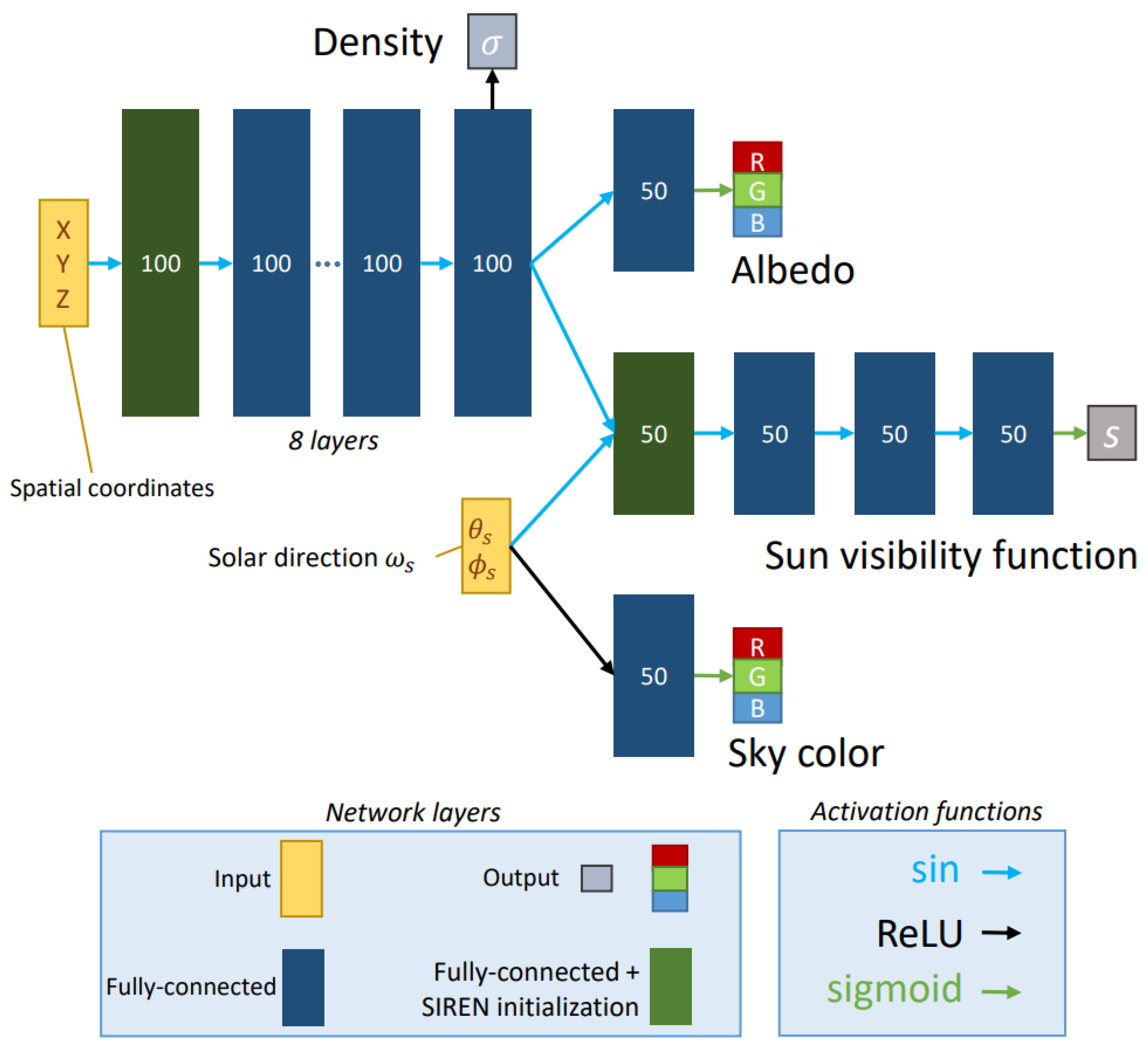
3.3. Network Architecture

The network architecture of RS-NeRF is shown in Figure 2, and is designed to be lightweight. RS-NeRF has only 20% of the neurons of S-NeRF, without additional branches. In order to shorten the query and training time of the network, float16 is used for all parameters.

3.3.1. HashEncoder

As shown in Figure 1, S-NeRF uses an 8-layer fully connected neural network to represent the scene’s geometric structure and three other branches to output albedo, sky color, and sun visibility. When a sampled point comes into the network, all neurons are involved in the computation for each query, which slows down the sampling efficiency.

Motivated by instant-NGP, we transfer the burden of scene representation to HashEncoder. We use the hash table instead of the neurons to store scene features. HashEncoder queries the features learned from the hash table by $(x,y,z)$ coordinate and feeds the queried features to the subsequent network. The hash table query is very fast, with time complexity of $O\left(1\right)$. Unlike neural networks, the hash table is computed with only the cell associated with the input point in each forward and backward propagation. This property not only significantly reduces the GPU memory footprint but also allows us to enhance the ability of scene representation by boosting the capacity of the hash table massively.

In particular, we turn the satellite image into a 24-level image pyramid, and each pixel in the image will have 24 sets of coordinates at different scales. We use the hash function(Equation (4)) to map the coordinates into hash values. Hash values are the addresses of cells, and we use them to look up the features in the corresponding cell.

$$h\left(\mathrm{x}\right)=\left(\underset{i=1}{\overset{3}{\oplus }}{x}_i{\pi }_i\right)modT$$

(4)

where ⊕ means the bit-wise XOR operation and T means the capacity of the hash table. When computing the multi-scale hash value for the input coordinates, the parameters of the hash function are set the same as in instant-NGP. We use the ${\pi }_1=1,{\pi }_2=19,349,663$, and ${\pi }_3=83,492,791$. We merge the 24 multi-scale hash features as the full features of the point and send them to the subsequent tiny network to predict the density and color of the point. The hash table has a large capacity of $2^{19}$ cells, updated by gradient descent. The query and the update only involve the cells associated with the input point. We will show in Experiment 4.2 that the hash table makes the network faster and the scene full of details.

3.3.2. Network Pruning

S-NeRF treats the point’s color as a combination of albedo and sky color (Equation (2)) and uses the sun visibility branch to find shadows. The sun visibility branch requires an additional batch for training. Three branches are complex, and we want to prune them. The network structure of RS-NeRF is shown in Figure 2. We remove the sun visibility and sky color branches. We feed the geometric structure features into the neural network with the solar direction and view direction to predict the color of the points. We use SHEncoder [44] for the solar direction and view direction, which helps to improve the result of the NeRF. The dropout layer [49] alleviates the network from overfitting shadows and vehicles. We demonstrate in Experiment 4.2 that RS-NeRF can still accurately distinguish shadows from building surfaces even after removing sun visibility.

3.4. Weights Sum Correction

In the same way as S-NeRF, we use Equation (5) to predict the altitude from the nadir view. We add a new L2 canonical term, weight sum correction, to the image reconstruction loss (Equation (6)) for better accuracy. This L2 canonical term encourages the sum of $w_i$ to be 1. We show in Experiment 4.4 that weight sum correction exhibits a tremendous gain in altitude estimation.

$$\widehat{h}=\sum _{i=1}^{N_s}{w}_i{h}_i,h_i\in [h_{max},h_{min}]$$

(5)

$$L\left(b\right)=\sum _{r\in b}\left({∥I\left(r\right)-\widehat{I}\left(r\right)∥}_2^2+{∥1-\sum _{i=1}^{N_s}{\omega }_i\left(r\right)∥}_2^2\right)$$

(6)

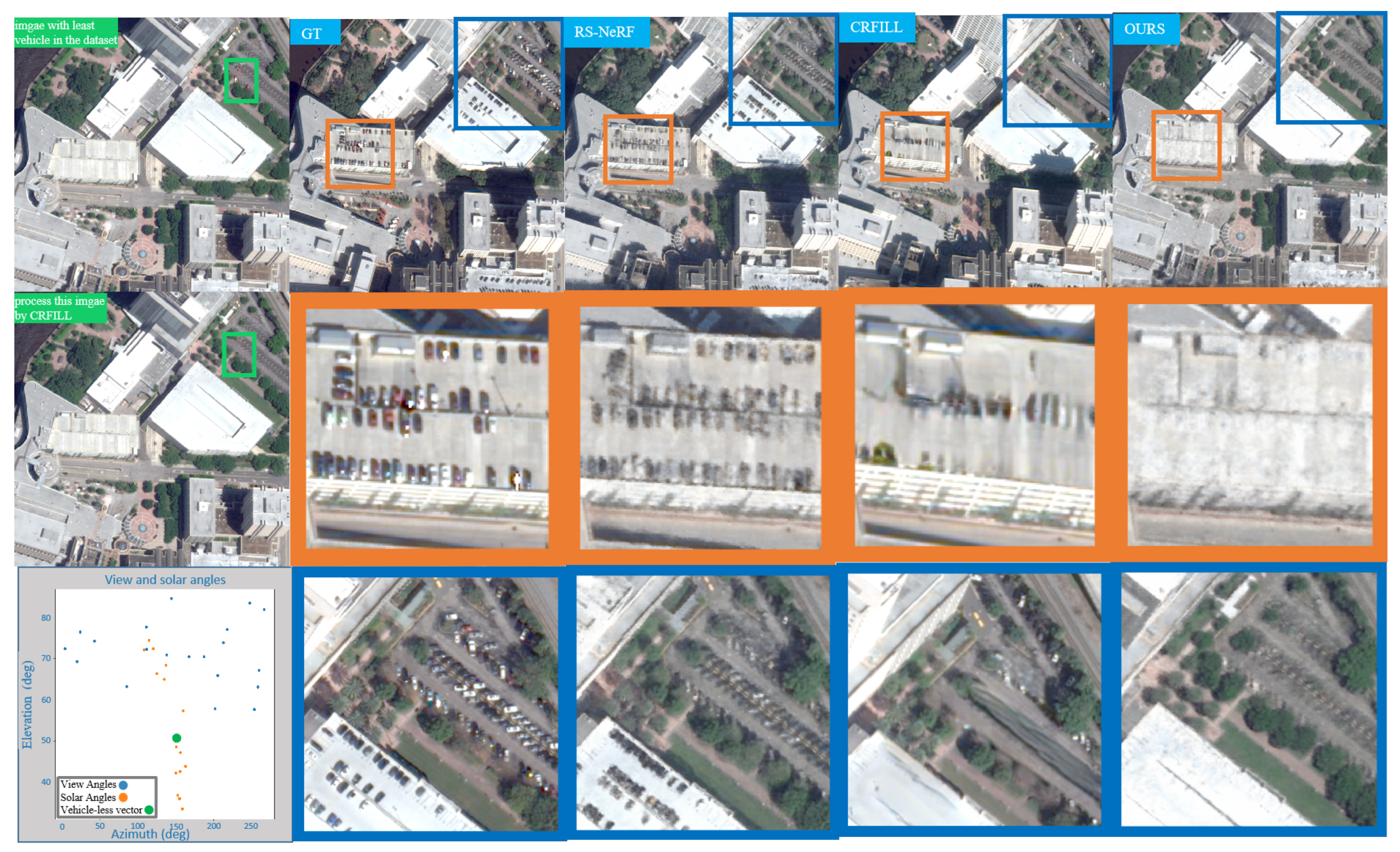
3.5. Vehicle Removal

The training images are not perfect because of the many randomly appearing vehicles. As shown in Figure 3, these dense vehicles affect people’s visual perception. For a better experience, we want to remove these cluttered and crowded vehicles and restore the original appearance of the city. We eliminate the vehicles in the scene by using the image-inpainting method to achieve this goal. Compared with other methods in this domain, CRFILL removes the attention module and block-by-block matching, so it has a small amount of computation and can complete the repair process quickly.

Directly using CRFILL to repair the whole training set brings a vast workload. Not only that, the error occurs when the road is entirely covered by vehicles (Figure 3). The structure of roads changes because CRFILL can only find the reference area within the input image. RS-NeRF, on the other hand, has a multi-view perceptual field and can avoid such a problem. Therefore we want to combine these two approaches.

The solar directions are different for each image in the training dataset (Figure 3). We can use the solar direction as a unique feature vector for each image and eliminate the artifacts caused by dense vehicles during RS-NeRF training (Figure 3). We select only one image to be processed by CRFILL, which contains the least number of vehicles in the training dataset (Figure 3). We save its corresponding solar direction as a vehicle-less vector. When synthesizing a new view image, the solar direction of the test image is replaced with the vehicle-less vector. We confirmed the feasibility of this idea in Experiment 4.3.

4. Experiments

4.1. Experimental Details

We evaluate our RS-NeRF method according to the experimental details of S-NeRF. RS-NeRF is evaluated on the WorldView-3 dataset collected between 2014 and 2016 over Jacksonville, Florida, USA [2]. From this dataset, we input a set of RGB crops of varying size, around 800 × 800 pixels, with a resolution of 0.3 m/pixel at the nadir. The number of train/test images and altitude bounds are listed in Table 1. We use airborne LiDAR maps as the ground truth to evaluate the performance of altitude extraction. RS-NeRF is trained with an Adam optimizer starting with a learning rate of 1 × 10${}^{-3}$. The batch size is 1024 rays, and each ray is discretized into 1024 uniformly distributed 3D points. Training takes 6 min on a single NVIDIA GPU with 12G RAM. The quantitative results of S-NeRF come from its paper, and we use the model weights provided by the author to generate visualization results for comparison. We will release our code soon.

The first experiment (Section 4.2) evaluates the performance of novel view synthesis. Then, we show how RS-NeRF can reconstruct the scene in the 160 s with high quality. The second experiment (Section 4.3) aims to remove the vehicles within the scene and restore the city to its original appearance. The third experiment (Section 4.4) evaluates the performance of altitude extraction and demonstrates the effect of the weight sum correction.

4.2. Novel View Synthesis

We compare the rendering results of the RS-NeRF and S-NeRF models from the unseen views and lighting conditions in Figure 4. Even after several hours of training, S-NeRF’s performance still needs to be improved. The RS-NeRF training time is only several minutes, with better performance. The turbine fan blades in the blue box and the parking spaces in the orange box demonstrate that RS-NeRF can accurately reproduce the details of the scene. The outputs of S-NeRF are over-smoothing and form a grayish area without crisp edges in this area. As seen from the green box, RS-NeRF can still render objects realistically in the shadows even without the sun visibility branch. The last row of ablation experiments proved that the HashEncoder is crucial for the success of RS-NeRF. Figure 5 shows how a scene RS-NeRF completes the reconstruction task within 160 s. Like an artist, RS-NeRF outlines the global scene in the first 5 s and then continuously refines it, a typical coarse-to-fine process. Figure 6 shows the performance of RS-NeRF on four different scenes after several minutes of training. Whether it is a vegetation-covered suburb or a crowded city block, RS-NeRF can show excellent reconstruction ability. We attempted to train RS-NeRF and S-NeRF using complete images of 2048 × 2048 pixel size as the training set. However, due to insufficient memory, S-NeRF could not be trained, and therefore, we only present the novel view synthesis results of RS-NeRF in Figure 7 and Table 1. It is worth noting that RS-NeRF exhibited good performance in a short period of time, without any changes to the model architecture and training parameters, except for some issues when dealing with ocean surfaces. Table 1 illustrates that the SSIM metric of RS-NeRF is far ahead in the limited training time. The drawback is that mass vehicles remain in the 068 scenes due to the influence of the training dataset, which looks terrible (Figure 3). We will address this problem in Experiment 4.3.

Figure 4. Urban details comparison. RS-NeRF demonstrated precise reproduction of roof details without excessive smoothing, as a result of synthesizing novel viewpoints in a densely built-up urban district. The HashEncoder plays a crucial role in RS-NeRF, and its removal would result in a significant degradation in quality.

Figure 4. Urban details comparison. RS-NeRF demonstrated precise reproduction of roof details without excessive smoothing, as a result of synthesizing novel viewpoints in a densely built-up urban district. The HashEncoder plays a crucial role in RS-NeRF, and its removal would result in a significant degradation in quality.

Figure 5. The reconstruction process of scene 068 in 160 s. Like an artist, RS-NeRF roughly depicts the whole scene in 5 s and then makes detailed adjustments.

Figure 5. The reconstruction process of scene 068 in 160 s. Like an artist, RS-NeRF roughly depicts the whole scene in 5 s and then makes detailed adjustments.

Figure 6. The novel view synthesis of RS-NeRF in 4 different scenes. Whether suburban or downtown, RS-NeRF can complete high-quality reconstruction in several minutes. In the 260 scenes, however, our results are missing a white building because the training set was collected at different years, and most of the training images are vacant lots or construction sites in this area. RS-NeRF tends to render this area as vacant lots.

Figure 6. The novel view synthesis of RS-NeRF in 4 different scenes. Whether suburban or downtown, RS-NeRF can complete high-quality reconstruction in several minutes. In the 260 scenes, however, our results are missing a white building because the training set was collected at different years, and most of the training images are vacant lots or construction sites in this area. RS-NeRF tends to render this area as vacant lots.

Figure 7. The high-resolution novel view synthesis results of RS-NeRF are impressive. Even when using full-sized images of 2048 × 2048 pixels as the training set and without changing the model structure or hyperparameters, RS-NeRF can still perform high-quality new view synthesis in just a few minutes. However, the SSIM values in Table 1 have decreased slightly, likely because of the significant differences in the appearance of the sea surface from different viewpoints, which RS-NeRF was unable to accurately learn.

Figure 7. The high-resolution novel view synthesis results of RS-NeRF are impressive. Even when using full-sized images of 2048 × 2048 pixels as the training set and without changing the model structure or hyperparameters, RS-NeRF can still perform high-quality new view synthesis in just a few minutes. However, the SSIM values in Table 1 have decreased slightly, likely because of the significant differences in the appearance of the sea surface from different viewpoints, which RS-NeRF was unable to accurately learn.

4.3. Vehicle Removal

In Experiment 4.2, many randomly appearing vehicles give scene 068 unpleasant reconstruction results (Figure 3). We attempt to eliminate the cars in training set to overcome this issue by CRFILL. However, some images contain too many cars, and using CRFILL directly to perform vehicle removal on them is labor-intensive and alters the scene’s geometric structure (Figure 3). Therefore, we only eliminate vehicles by CRFILL in the image with the fewest cars from the training set (Figure 3), dramatically decreasing the burden and assuring that the scene’s appearance remains unchanged. When generating the new view images, we send the solar direction of the processed image as a vehicle-less vector into the network. RS-NeRF can clear the vehicles in the orange box, whereas CRFILL leaves some artifacts. In the blue box, CRFILL distorts the road when the cars obstruct the road, because CRFILL’s perceptual field is limited to a single image. When the road is completely obscured, it is difficult for the algorithm to find the reference area used to fix the obscuration from the image. However, our RS-NeRF has a global perceptual field and can adaptively find the corresponding area as a reference from the perfect unobstructed view. This experiment demonstrates that the vehicle-less property of the proposed image can be transmitted through the solar angle, leaving the scene clean.

4.4. Altitude Extraction

We evaluated the altitude extraction performance of RS-NeRF in this experiment. We followed S-NeRF’s method of projecting the rays from the nadir, obtaining a rendered vertical view, and calculating the average error between the estimation results and the LiDAR. The height is calculated using Equation (5). To estimate the height more accurately, we add a new regular term in Equation (6) during the training process, which encourages the weights of points on the same ray to sum to 1. We ablate the regular term in four different scenes. Table 1 and Figure 8 show the significant improvement by our regular term without additional time overhead.

Figure 9 compares the altitude extraction results of RS-NeRF and S-NeRF. By observing the blue and green boxes, we can find that RS-NeRF is comparable to LiDAR and can accurately represent the fine structure of the building. In the orange box, RS-NeRF has more details than the LiDAR results. Table 1 further demonstrates from a quantitative perspective that RS-NeRF can obtain outstanding results in a very short time.

5. Conclusions

In this paper, we propose a new NeRF variant for multi-view satellite photogrammetry, which can extract accurate altitude maps from optical images and quickly render photo-realistic novel view images. First, we design an efficient adaptive sampling method with custom CUDA kernels to accelerate the solution of the volumetric rendering formulation. Second, the lightweight network with HashEncoder is designed to learn the 3D scene full of details sufficiently. Third, our approach combines the latest research in image inpainting to eliminate artifacts from dense vehicles. Moreover, we add the weight sum correction to the loss function for more accurate altitude prediction with MAEs of about 2 m.

References

1. Hlatshwayo, S.T.; Mutanga, O.; Lottering, R.T.; Kiala, Z.; Ismail, R. Mapping forest aboveground biomass in the reforested Buffelsdraai landfill site using texture combinations computed from SPOT-6 pan-sharpened imagery. Int. J. Appl. Earth Obs. Geoinf. 2019, 74, 65–77. [Google Scholar] [CrossRef]
2. Le Saux, B.; Yokoya, N.; Hänsch, R.; Brown, M. 2019 ieee grss data fusion contest: Large-scale semantic 3d reconstruction. IEEE Geosci. Remote Sens. Mag. (GRSM) 2019, 7, 33–36. [Google Scholar] [CrossRef]
3. Gwinner, K.; Jaumann, R.; Hauber, E.; Hoffmann, H.; Heipke, C.; Oberst, J.; Neukum, G.; Ansan, V.; Bostelmann, J.; Dumke, A.; et al. The High Resolution Stereo Camera (HRSC) of Mars Express and its approach to science analysis and mapping for Mars and its satellites. Planet. Space Sci. 2016, 126, 93–138. [Google Scholar] [CrossRef]
4. Simard, M.; Zhang, K.; Rivera-Monroy, V.H.; Ross, M.S.; Ruiz, P.L.; Castañeda-Moya, E.; Twilley, R.R.; Rodriguez, E. Mapping height and biomass of mangrove forests in Everglades National Park with SRTM elevation data. Photogramm. Eng. Remote Sens. 2006, 72, 299–311. [Google Scholar] [CrossRef]
5. Demarez, V.; Helen, F.; Marais-Sicre, C.; Baup, F. In-season mapping of irrigated crops using Landsat 8 and Sentinel-1 time series. Remote Sens. 2019, 11, 118. [Google Scholar] [CrossRef] [Green Version]
6. Qin, R.; Tian, J.; Reinartz, P. 3D change detection–approaches and applications. ISPRS J. Photogramm. Remote Sens. 2016, 122, 41–56. [Google Scholar] [CrossRef] [Green Version]
7. Hirschmuller, H. Stereo processing by semiglobal matching and mutual information. IEEE Trans. Pattern Anal. Mach. Intell. 2007, 30, 328–341. [Google Scholar] [CrossRef]
8. d’Angelo, P.; Kuschk, G. Dense multi-view stereo from satellite imagery. In Proceedings of the 2012 IEEE International Geoscience and Remote Sensing Symposium, Munich, Germany, 22–27 July 2012; pp. 6944–6947. [Google Scholar]
9. De Franchis, C.; Meinhardt-Llopis, E.; Michel, J.; Morel, J.M.; Facciolo, G. An automatic and modular stereo pipeline for pushbroom images. ISPRS Ann. Photogramm. Remote Sens. Spatial Inf. Sci. 2014, 2, 49–56. [Google Scholar] [CrossRef] [Green Version]
10. Facciolo, G.; De Franchis, C.; Meinhardt-Llopis, E. Automatic 3D reconstruction from multi-date satellite images. In Proceedings of the IEEE Conference on Computer Vision and Pattern Recognition Workshops, Honolulu, HI, USA, 21–27 July 2017; pp. 57–66. [Google Scholar]
11. Gong, K.; Fritsch, D. DSM generation from high resolution multi-view stereo satellite imagery. Photogramm. Eng. Remote Sens. 2019, 85, 379–387. [Google Scholar] [CrossRef]
12. Rupnik, E.; Pierrot-Deseilligny, M.; Delorme, A. 3D reconstruction from multi-view VHR-satellite images in MicMac. ISPRS J. Photogramm. Remote Sens. 2018, 139, 201–211. [Google Scholar] [CrossRef]
13. Shean, D.E.; Alexandrov, O.; Moratto, Z.M.; Smith, B.E.; Joughin, I.R.; Porter, C.; Morin, P. An automated, open-source pipeline for mass production of digital elevation models (DEMs) from very-high-resolution commercial stereo satellite imagery. ISPRS J. Photogramm. Remote Sens. 2016, 116, 101–117. [Google Scholar] [CrossRef]
14. Marí, R.; Facciolo, G.; Ehret, T. Sat-NeRF: Learning Multi-View Satellite Photogrammetry with Transient Objects and Shadow Modeling Using RPC Cameras. In Proceedings of the IEEE/CVF Conference on Computer Vision and Pattern Recognition, New Orleans, LA, USA, 18–24 June 2022; pp. 1311–1321. [Google Scholar]
15. Mildenhall, B.; Srinivasan, P.P.; Tancik, M.; Barron, J.T.; Ramamoorthi, R.; Ng, R. Nerf: Representing scenes as neural radiance fields for view synthesis. Commun. ACM 2021, 65, 99–106. [Google Scholar] [CrossRef]
16. Barron, J.T.; Mildenhall, B.; Tancik, M.; Hedman, P.; Martin-Brualla, R.; Srinivasan, P.P. Mip-nerf: A multiscale representation for anti-aliasing neural radiance fields. In Proceedings of the IEEE/CVF International Conference on Computer Vision, Montreal, QC, Canada, 10–17 October 2021; pp. 5855–5864. [Google Scholar]
17. Martin-Brualla, R.; Radwan, N.; Sajjadi, M.S.; Barron, J.T.; Dosovitskiy, A.; Duckworth, D. Nerf in the wild: Neural radiance fields for unconstrained photo collections. In Proceedings of the IEEE/CVF Conference on Computer Vision and Pattern Recognition, Nashville, TN, USA, 20–25 June 2021; pp. 7210–7219. [Google Scholar]
18. Park, K.; Sinha, U.; Barron, J.T.; Bouaziz, S.; Goldman, D.B.; Seitz, S.M.; Martin-Brualla, R. Nerfies: Deformable neural radiance fields. In Proceedings of the IEEE/CVF International Conference on Computer Vision, Montreal, QC, Canada, 10–17 October 2021; pp. 5865–5874. [Google Scholar]
19. Li, W.; Pan, C.; Zhang, R.; Ren, J.; Ma, Y.; Fang, J.; Yan, F.; Geng, Q.; Huang, X.; Gong, H.; et al. AADS: Augmented autonomous driving simulation using data-driven algorithms. Sci. Robot. 2019, 4, eaaw0863. [Google Scholar] [CrossRef] [PubMed]
20. Ost, J.; Mannan, F.; Thuerey, N.; Knodt, J.; Heide, F. Neural scene graphs for dynamic scenes. In Proceedings of the IEEE/CVF Conference on Computer Vision and Pattern Recognition, Nashville, TN, USA, 20–25 June 2021; pp. 2856–2865. [Google Scholar]
21. Yang, Z.; Chai, Y.; Anguelov, D.; Zhou, Y.; Sun, P.; Erhan, D.; Rafferty, S.; Kretzschmar, H. Surfelgan: Synthesizing realistic sensor data for autonomous driving. In Proceedings of the IEEE/CVF Conference on Computer Vision and Pattern Recognition, Seattle, WA, USA, 13–19 June 2020; pp. 11118–11127. [Google Scholar]
22. Du, D.; Qi, Y.; Yu, H.; Yang, Y.; Duan, K.; Li, G.; Zhang, W.; Huang, Q.; Tian, Q. The unmanned aerial vehicle benchmark: Object detection and tracking. In Proceedings of the European Conference on Computer Vision (ECCV), Munich, Germany, 8–14 September 2018; pp. 370–386. [Google Scholar]
23. Liu, A.; Tucker, R.; Jampani, V.; Makadia, A.; Snavely, N.; Kanazawa, A. Infinite nature: Perpetual view generation of natural scenes from a single image. In Proceedings of the IEEE/CVF International Conference on Computer Vision, Montreal, QC, Canada, 10–17 October 2021; pp. 14458–14467. [Google Scholar]
24. Deng, K.; Liu, A.; Zhu, J.Y.; Ramanan, D. Depth-supervised nerf: Fewer views and faster training for free. In Proceedings of the IEEE/CVF Conference on Computer Vision and Pattern Recognition, New Orleans, LA, USA, 18–24 June 2022; pp. 12882–12891. [Google Scholar]
25. Tancik, M.; Casser, V.; Yan, X.; Pradhan, S.; Mildenhall, B.; Srinivasan, P.P.; Barron, J.T.; Kretzschmar, H. Block-nerf: Scalable large scene neural view synthesis. In Proceedings of the IEEE/CVF Conference on Computer Vision and Pattern Recognition, New Orleans, LA, USA, 18–24 June 2022; pp. 8248–8258. [Google Scholar]
26. Rematas, K.; Liu, A.; Srinivasan, P.P.; Barron, J.T.; Tagliasacchi, A.; Funkhouser, T.; Ferrari, V. Urban radiance fields. In Proceedings of the IEEE/CVF Conference on Computer Vision and Pattern Recognition, New Orleans, LA, USA, 18–24 June 2022; pp. 12932–12942. [Google Scholar]
27. Derksen, D.; Izzo, D. Shadow neural radiance fields for multi-view satellite photogrammetry. In Proceedings of the IEEE/CVF Conference on Computer Vision and Pattern Recognition, Nashville, TN, USA, 20–25 June 2021; pp. 1152–1161. [Google Scholar]
28. Müller, T.; Evans, A.; Schied, C.; Keller, A. Instant neural graphics primitives with a multiresolution hash encoding. arXiv 2022, arXiv:2201.05989. [Google Scholar] [CrossRef]
29. Agarwal, S.; Furukawa, Y.; Snavely, N.; Simon, I.; Curless, B.; Seitz, S.M.; Szeliski, R. Building rome in a day. Commun. ACM 2011, 54, 105–112. [Google Scholar] [CrossRef]
30. Früh, C.; Zakhor, A. An automated method for large-scale, ground-based city model acquisition. Int. J. Comput. Vis. 2004, 60, 5–24. [Google Scholar] [CrossRef] [Green Version]
31. Li, X.; Wu, C.; Zach, C.; Lazebnik, S.; Frahm, J.M. Modeling and recognition of landmark image collections using iconic scene graphs. In Proceedings of the Computer Vision–ECCV 2008: 10th European Conference on Computer Vision, Marseille, France, 12–18 October 2008; pp. 427–440. [Google Scholar]
32. Pollefeys, M.; Nistér, D.; Frahm, J.M.; Akbarzadeh, A.; Mordohai, P.; Clipp, B.; Engels, C.; Gallup, D.; Kim, S.J.; Merrell, P.; et al. Detailed real-time urban 3d reconstruction from video. Int. J. Comput. Vis. 2008, 78, 143–167. [Google Scholar] [CrossRef] [Green Version]
33. Snavely, N.; Seitz, S.M.; Szeliski, R. Photo tourism: Exploring photo collections in 3D. In ACM Siggraph 2006 Papers; Association for Computing Machinery: New York, NY, USA, 2006; pp. 835–846. [Google Scholar]
34. Zhu, S.; Zhang, R.; Zhou, L.; Shen, T.; Fang, T.; Tan, P.; Quan, L. Very large-scale global sfm by distributed motion averaging. In Proceedings of the IEEE Conference on Computer Vision and Pattern Recognition, Salt Lake City, UT, USA, 18–23 June 2018; pp. 4568–4577. [Google Scholar]
35. Schonberger, J.L.; Frahm, J.M. Structure-from-motion revisited. In Proceedings of the IEEE Conference on Computer Vision and Pattern Recognition, Las Vegas, NV, USA, 27–30 June 2016; pp. 4104–4113. [Google Scholar]
36. Lowe, D.G. Distinctive image features from scale-invariant keypoints. Int. J. Comput. Vis. 2004, 60, 91–110. [Google Scholar] [CrossRef]
37. Beyer, R.A.; Alexandrov, O.; McMichael, S. The Ames Stereo Pipeline: NASA’s open source software for deriving and processing terrain data. Earth Space Sci. 2018, 5, 537–548. [Google Scholar] [CrossRef]
38. Rupnik, E.; Deseilligny, M.P. More surface detail with One-Two-Pixel Matching. Ph.D. Thesis, Institut Géographique National (IGN), Saint-Mandé, France, 2019. [Google Scholar]
39. Liu, L.; Gu, J.; Zaw Lin, K.; Chua, T.S.; Theobalt, C. Neural sparse voxel fields. Adv. Neural Inf. Process. Syst. 2020, 33, 15651–15663. [Google Scholar]
40. Park, J.J.; Florence, P.; Straub, J.; Newcombe, R.; Lovegrove, S. Deepsdf: Learning continuous signed distance functions for shape representation. In Proceedings of the IEEE/CVF Conference on Computer Vision and Pattern Recognition, Long Beach, CA, USA, 15–20 June 2019; pp. 165–174. [Google Scholar]
41. Lombardi, S.; Simon, T.; Saragih, J.; Schwartz, G.; Lehrmann, A.; Sheikh, Y. Neural volumes: Learning dynamic renderable volumes from images. arXiv 2019, arXiv:1906.07751. [Google Scholar] [CrossRef] [Green Version]
42. Tewari, A.; Thies, J.; Mildenhall, B.; Srinivasan, P.; Tretschk, E.; Yifan, W.; Lassner, C.; Sitzmann, V.; Martin-Brualla, R.; Lombardi, S.; et al. Advances in neural rendering. In Computer Graphics Forum; Wiley: Hoboken, NJ, USA, 2022; Volume 41, pp. 703–735. [Google Scholar]
43. Xiangli, Y.; Xu, L.; Pan, X.; Zhao, N.; Rao, A.; Theobalt, C.; Dai, B.; Lin, D. Bungeenerf: Progressive neural radiance field for extreme multi-scale scene rendering. In Proceedings of the Computer Vision–ECCV 2022: 17th European Conference, Tel Aviv, Israel, 23–27 October 2022; pp. 106–122. [Google Scholar]
44. Yu, A.; Li, R.; Tancik, M.; Li, H.; Ng, R.; Kanazawa, A. Plenoctrees for real-time rendering of neural radiance fields. In Proceedings of the IEEE/CVF International Conference on Computer Vision, Montreal, QC, Canada, 10–17 October 2021; pp. 5752–5761. [Google Scholar]
45. Yang, B.; Zhang, Y.; Xu, Y.; Li, Y.; Zhou, H.; Bao, H.; Zhang, G.; Cui, Z. Learning object-compositional neural radiance field for editable scene rendering. In Proceedings of the IEEE/CVF International Conference on Computer Vision, Montreal, QC, Canada, 10–17 October 2021; pp. 13779–13788. [Google Scholar]
46. Zhang, J.; Liu, X.; Ye, X.; Zhao, F.; Zhang, Y.; Wu, M.; Zhang, Y.; Xu, L.; Yu, J. Editable free-viewpoint video using a layered neural representation. ACM Trans. Graph. (TOG) 2021, 40, 1–18. [Google Scholar]
47. Zeng, Y.; Lin, Z.; Lu, H.; Patel, V.M. Cr-fill: Generative image inpainting with auxiliary contextual reconstruction. In Proceedings of the IEEE/CVF International Conference on Computer Vision, Montreal, QC, Canada, 10–17 October 2021; pp. 14164–14173. [Google Scholar]
48. Krauß, T.; d’Angelo, P.; Wendt, L. Cross-track satellite stereo for 3D modelling of urban areas. Eur. J. Remote Sens. 2019, 52, 89–98. [Google Scholar] [CrossRef] [Green Version]
49. Srivastava, N.; Hinton, G.; Krizhevsky, A.; Sutskever, I.; Salakhutdinov, R. Dropout: A simple way to prevent neural networks from overfitting. J. Mach. Learn. Res. 2014, 15, 1929–1958. [Google Scholar]
Figure 1. The network of S-NeRFs. The fully-connected layers are used to learn the color and the density of the whole scene. The network takes spatial coordinates ( x , y , z ) and solar direction ω s , then outputs the color, density and sun visibility. The pixel values in the rendered image is the weighted sum of these outputs (Equation (1)). The sun visibility branch requires a separate batch for training, which brings additional time overhead.
Remotesensing 15 03808 g001
Figure 2. The network of RS-NeRF. The input consists of the sampled point’s coordinate, the direction of observation, and the sunshine angle. The output is the point’s density and color. RS-NeRF uses fewer neurons and eliminates unnecessary branches compared to S-NeRF (Figure 1).
Remotesensing 15 03808 g002
Figure 3. The result of vehicle removal. Random vehicles give RS-NeRF unpleasant reconstruction results. CRFILL does not perform well on images with dense vehicles. We select only one image to be processed by CRFILL, which contains the least number of vehicles in the training dataset. Then we save its solar angels as the vehicle-less vector. When synthesizing a new view image, the solar direction of the test image is replaced with the vehicle-less vector. Compared to CRFILL, our method can eliminate these artifacts and maintain the correct geometry.
Remotesensing 15 03808 g003
Figure 8. The performance of altitude extraction from four different areas. These altitude maps correspond to the MAE in Table 1.
Remotesensing 15 03808 g008
Figure 9. The results of altitude extraction of scene 068. We use the model weights provided by the author to generate visualization results for comparison. Looking at the blue and yellow boxes, we notice that the structure from RS-NeRF is more precise and detailed than S-NeRF. Moreover, in the orange box, RS-NeRF shows more details than LiDAR.
Remotesensing 15 03808 g009