A Super-Resolution Algorithm Based on Hybrid Network for Multi-Channel Remote Sensing Images

Abstract

In recent years, the development of super-resolution (SR) algorithms based on convolutional neural networks has become an important topic in enhancing the resolution of multi-channel remote sensing images. However, most of the existing SR models suffer from the insufficient utilization of spectral information, limiting their SR performance. Here, we derive a novel hybrid SR network (HSRN) which facilitates the acquisition of joint spatial–spectral information to enhance the spatial resolution of multi-channel remote sensing images. The main contributions of this paper are three-fold: (1) in order to sufficiently extract the spatial–spectral information of multi-channel remote sensing images, we designed a hybrid three-dimensional (3D) and two-dimensional (2D) convolution module which can distill the nonlinear spectral and spatial information simultaneously; (2) to enhance the discriminative learning ability, we designed the attention structure, including channel attention, before the upsampling block and spatial attention after the upsampling block, to weigh and rescale the spectral and spatial features; and (3) to acquire fine quality and clear texture for reconstructed SR images, we introduced a multi-scale structural similarity index into our loss function to constrain the HSRN model. The qualitative and quantitative comparisons were carried out in comparison with other SR methods on public remote sensing datasets. It is demonstrated that our HSRN outperforms state-of-the-art methods on multi-channel remote sensing images.

1. Introduction

Remote sensing images are being increasingly widely utilized in various fields, such as target characteristic analysis [1], detection [2], and classification [3,4]. However, due to the trade-off between spectral and spatial resolution, the multi-channel images have a coarse spatial resolution, limiting their further development. Super-resolution (SR) approaches, which directly reconstruct high-resolution (HR) images from low-resolution (LR) images, play a vital role in resolution enhancement and are meaningful for the practical application of remote sensing images. How to design an effective SR model for remote sensing images is the focus of this research paper.

Numerous SR models have been proposed in recent years and can be classified into two types: multi-image SR models (MISR) and single-image SR models (SISR). For the first type, models [5,6,7] employed diverse methods by fusing multi-remote sensing images to improve the spatial resolution. Dian et al. [5] learned a spectral dictionary from multi-spectral and hyperspectral images to produce sparse representations for enhancing the resolution. In [6], Liu et al. applied a two-stream fusion network to enhance the resolution of multi-spectral images combined with panchromatic images. Huang et al. [7] proposed a compact step-wise fusing strategy by incorporating multi-spectral and panchromatic images into a framework to favor the resolution improvement in hyperspectral images. These models achieved a remarkable SR performance for remote sensing images due to the additional fused data. However, the reconstructed results of multi-image SR models are sensitive for geometric correction and time variations, limiting their further applications.

The SISR models concentrate on creating powerful models to extract features from a single image. The reconstructed images using SISR [8] can be applied for many other applications, such as target tracking [9] and disparity map generation [10]. Most existing SISRs can be roughly categorized into hand-crafted models and end-to-end models [11]. For the former, each step of these methods is manually designed with good interpretability. Interpolation-based models such as bilinear and bicubic models [12] are a kind of hand-crafted SR model which have been widely applied in remote sensing production. Earlier studies have worked on optimizing linear regression models to improve their reconstruction performance. Ma et al. [13] proposed a robust local kernel regression approach to enhance the spatial resolution of multi-angle remote sensing images. In [14], Schulter et al. also presented a locally linear model which employed random forests for mapping LR images into HR images. Timofte et al. [15] summarized seven techniques which are widely applicable in SISR methods. These models have an intuitive structure and can quickly enhance the resolution, but suffer from a serious problem of quality degradation after reconstruction. Sparse representation-based models are another type of hand-crafted SR model which flexibly combine atoms and elements [16] to reconstruct HR images. Peleg and Elad [17] designed a dictionary pair model by extracting the sparse coefficients of HR and LR images to improve the resolution. In [18], Hou et al. explored a global joint dictionary model to sufficiently obtain the global and local information of remote sensing images. To increase the representation ability of sparse decomposition, Shao et al. [19] applied a coupled sparse autoencoder to effectively map LR images into HR images. However, these models carry huge computational expense for sparsity constraint, which may have a minimal effect on image representation [20,21]. More importantly, the sparsity-based SISR models suffer from the weakness of extracting deep features, restricting their reconstruction precision.

End-to-end models are composed of various networks [22] in which parameters can be automatically updated by forward and afterward propagation. These models [18,19,20,21,22,23,24,25,26,27] are designed for natural images, which provide references for the SR task of remote sensing images. Patil et al. [23] proposed using a neural network to extract the structural correlation and predict fine details of reconstructed images. Su et al. [24] combined a Hopfield neural network and contouring to enhance the super resolution of remote sensing images. In recent years, convolutional neural networks (CNNs) have been widely used to enhance the resolution of images. The pioneering study [25] employed a CNN to improve the resolution, and achieved a better performance than hand-crafted ones. Shi et al. [26] designed an efficient sub-pixel convolutional network (ESPCN) which introduced a pixel-shuffle layer to reduce the computation complexity. In [27], Kim et al. used a residual-learning module and designed a very deep SR model (VDSR) to reconstruct HR images. A deeper model named a residual dense network (RDN) [28] was constructed to make full use of the hierarchical features from the LR images and produce a better trade-off between efficiency and effectiveness in recovering the HR images. These models fully exploited spatial information to improve the resolution, but they ignored the internal relations between different channels. In [29], Zhang et al. designed residual channel attention networks to weigh the spectral band and built an SR model named a residual channel attention network (RCAN). Basak et al. [30] optimized an RCAN model and applied it to enhance single-image resolution. In [31], Mei et al. explored the effects of cross-scale spatial information on SR requirements and proposed a cross-scale non-local network (CSNLN). It introduced the non-local priors into framework for extracting multi-scale features within an LR image. Xia et al. [32] built an architecture called an efficient non-local contrastive network (ENLCN). This model consists of non-local attention and a sparse aggregation module to further strengthen the effect of relevant features. However, these models are not designed for multi-channel remote sensing images and fail to extract nonlinear spectral information.

Inspired by the aforementioned approaches, a great number of SR models for remote sensing images were proposed. Mei et al. [33] constructed a three-dimensional full convolutional neural network (3D-FCNN) for multi-spectral and hyperspectral images. This model exploited both the spatial neighboring pixels and spectral bands without sufficient distinction between interesting and uninteresting information. Li et al. [34] proposed a gradient-guided group-attention network to map LR images into HR images. The gradient information was introduced in the reconstruction framework to promote sharp edges and realistic textures. This strategy causes texture distortion when it enhances resolution on a small scale. In [35], Wang et al. employed a recurrent feedback network to exploit the spatial–spectral information. They introduced a group strategy for spectral channels which destroyed the structure of the spectral curve. Lei and Shi [36] designed a hybrid-scale self-similarity exploitation network (HSENet) which used different scales’ similarities to enhance the remote sensing images. Then, they designed the transformer-based enhancement network (TranENet) [37] which applied the transformers to fuse multi-scale features for image enhancement. The multi-scale self-similarity exploitation provides abundant textures for reconstructed images, but they ignore spectral features. Deng et al. [38] designed a multiple-frame splicing strategy to enhance the resolution of hyperspectral images. However, this model focuses on improving distorted images, limiting the stability of the spectral information in the reconstructed images.

Generally, the adjacent spectral bands and spatial pixels in multi- or hyperspectral remote sensing images are correlated [39]. To fully extract interesting spatial-spectral information, we designed a novel algorithm named the hybrid SR network (HSRN) to map the LR multi-channel (channel number ≥ 3) remote sensing images into HR images. Specifically, we designed a hybrid module consisting of three-dimensional (3D) and two-dimensional (2D) convolutional layers to extract the nonlinear information of the spectral and spatial domains. Additionally, to exploit the inherent differences and interdependence across feature maps, we introduced channel (spectral) and spatial attention mechanisms, which prompt an increase in discriminative learning ability. We employed a sub-pixel upsampling module (pixel-shuffle layer) to recombine the feature maps to enhance the resolution of the images. In the end, we applied the joint loss function to constrain the model and recover the images with the most accurate texture and spectra possible, compared with label maps. We tested our model on three public datasets and calculated three evaluation metrics to assess the performance of the SR methods. The experimental results prove that our model outperforms state-of-the-art models. The main contributions of this article can be summarized as follows.

(1)

We propose a novel hybrid SR model combining 3D and 2D convolutional networks for multi-channel images. The improvement encourages our model to capture the spatial and spectral information simultaneously, and fully utilizes the different responses of various channels to enhance the spatial resolution.

(2)

We designed an attention structure to strengthen the SR performance for multi-channel images. We applied channel attention to learn the inter-band correlation before the upsampling block and employed spatial attention to refine the spatial texture of the upsampling feature maps.

(3)

We introduced multi-scale structural similarity (MS-SSIM) into our loss function to constrain the proposed model and acquire a rich texture. The MS-SSIM function forces our model to learn the multi-scale structure from labels and reconstruct high-quality HR images.

The organization of this article is as follows. In Section 2, we present the related works on SR models. Section 3 depicts the details of our proposed algorithm for multi-channel remote sensing images. The experimental consequences and the analysis of the public datasets are exhibited in Section 4. Conclusions are drawn in Section 5.

2. Related Works

In recent decades, CNN frameworks have been shown to be highly successful in remote sensing imagery augmentation [40]. These models are capable of directly extracting abundant characteristics from large volumes of realistic images. The attention mechanism is an important component of CNN models that can enhance the discriminative ability of the model to depict rich scenes from remote sensing images. In this subsection, we focus on works related to CNN-based SR models and the attention mechanism.

2.1. CNN for SR without Attention Mechanism

This pioneer method was proposed by Dong et al. [25]. It employed three-layer convolutional networks to increase the resolution and achieved a remarkable performance compared to traditional methods. Along with the proposal of residual blocks [41], SR models made continuous progress in the algorithm’s architecture. Kim et al. [27] designed a 20-layer residual network which acquired significant improvement in reconstruction accuracy. A faster SR network [42] was designed to map LR images into HR images and accelerate the training and test process. Lim et al. [43] built an enhanced deep super-resolution (EDSR) network which removed batch normalization layers and adopted a deep convolutional structure to improve the resolution. Shi et al. [44] adopted a 160-/240-layer network consisting of standard residual blocks to recover HR hyperspectral images. However, simply stacking residual blocks to construct a very deep network can hardly result in improvement. The attention mechanism is an alternative strategy to improve the representation ability of SR models. Tian et al. [45] proposed a coarse-to-fine SR network, consisting of a 46-layer convolution, to reconstruct a high-resolution (HR) image. The network includes feature extraction blocks, an enhancement block, a construction block, and a feature refinement block. They designed a feature fusion scheme to prevent information loss and introduced a cascaded network that combines LR and HR features to mitigate potential training instability and performance degradation. Huan et al. [22] designed a pyramidal multi-scale residual network that consists of a feature extraction part and a reconstruction part. The feature extraction part utilized dilation convolution to enhance the ability to detect contextual information, while employing hierarchical residual-like connections to fuse multi-scale features. The reconstruction part employed a complementary block of global and local features to address the issue of useful original information being ignored.

2.2. CNN for SR with Attention Mechanism

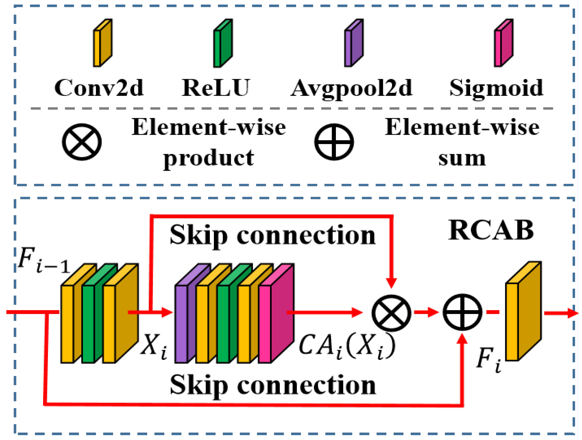
The attention mechanism encourages learning models to focus on the prominent features [46] between the spatial and spectral domains. Zhang et al. [29] introduced the channel attention block and constructed a residual channel attention block (RCAB). As shown in Figure 1, the RCAB applies a long skip connection to deliver the main signal and channel attention to weigh different feature maps. The skip connection encourages the network to focus on the high-frequency signal of the LR feature maps. Suppose that the i-th output and input of the RCAB are $F_i$ and $F_{i-1}$. The calculation of the RCAB is as follows:

$$F_i=F_{i-1}+{CA}_i\left(X_i\right)·X_i,$$

(1)

where ${CA}_i$ denotes the function of the channel attention and $X_i$ is the residual signal produced by two stacked convolution layers from $F_{i-1}$. This block fully captures the channel-wise dependencies and is essential to multi-channel remote sensing images containing varied spatial and spectral information. However, it ignores the nonlinear spectral information, which is important for the SR task of remote sensing images. Jiang et al. [47] designed a cross-dimension attention network to improve the resolution of remote sensing images. While considering the interactivity between the channel and spatial dimensions, they overlooked the extraction of nonlinear spectral information from multi-channel remote sensing images. In [48], Li et al. designed a 3D-RCAB to extract abundant spatial and spectral information to enhance the spectrum. However, the 3D-RCAB is complex and time consuming, and suffers from the weakness of extracting prominent spatial information. Therefore, we explored an efficient 3D–2D hybrid network to recover the HR images, and designed a spectral and spatial attention structure to improve the representational power of the network.

3. Materials and Methods

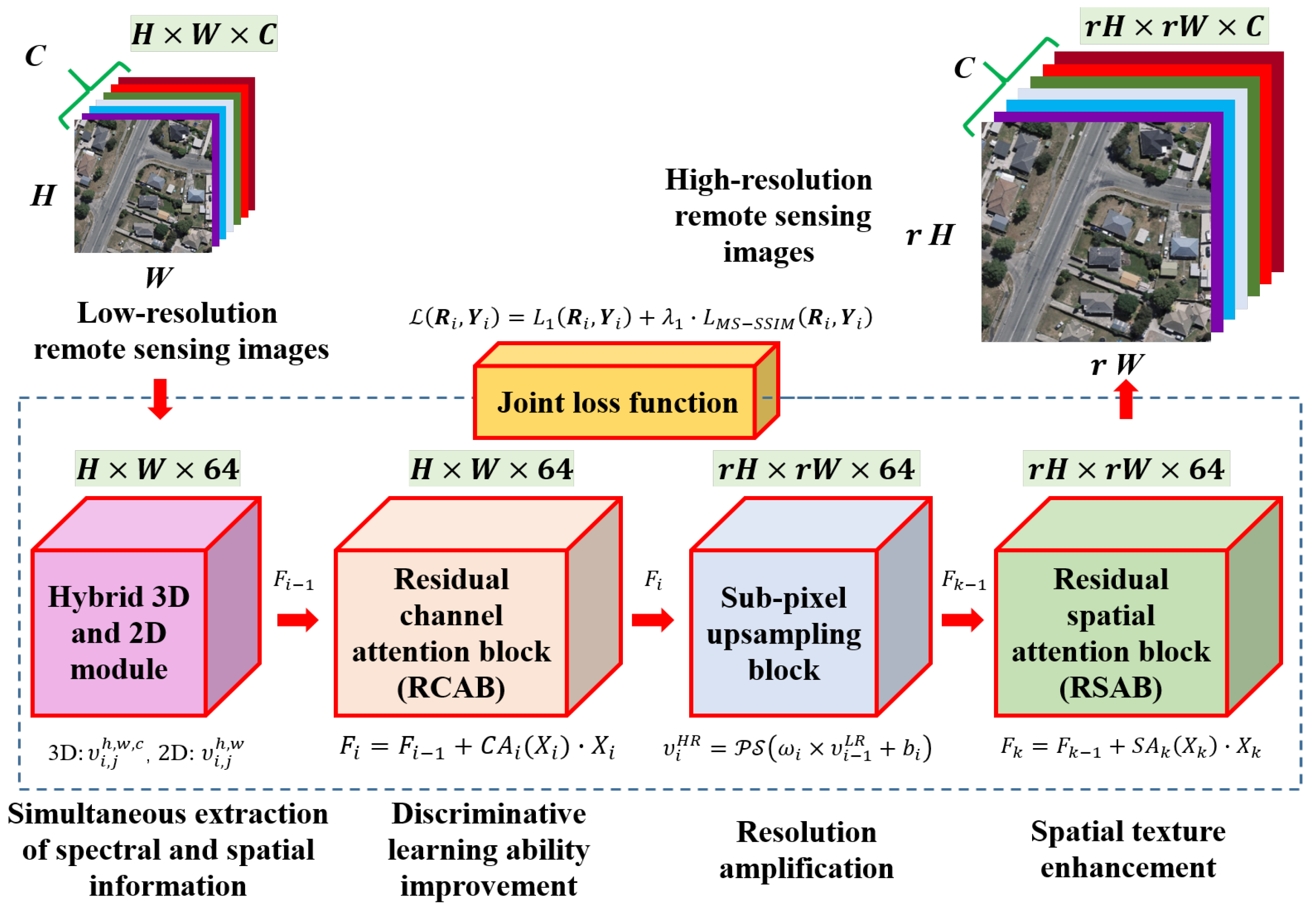
The flowchart of the proposed HSRN is illustrated in Figure 2. The LR remote sensing images are first input into the hybrid 3D–2D module to extract the abundant spatial–spectral information. Then, an RCAB is employed to learn and represent the acquired feature maps for improving the discriminative ability of the SR model. Moreover, the sub-pixel upsampling block is adopted to enhance the resolution of the incoming feature maps. Finally, the reconstructed feature maps are refined by our residual spatial attention block (RSAB) and turned into HR remote sensing images. The whole framework is constrained by a joint loss function and can be converged quickly.

3.1. Hybrid 3D–2D Module

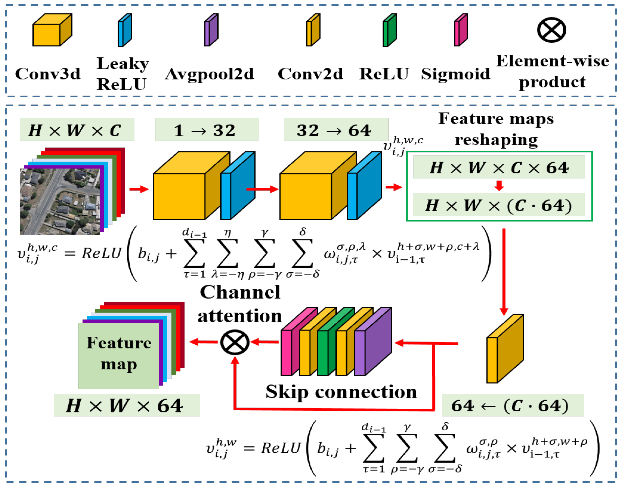
Let the multi-channel remote sensing cube be denoted by $\mathbf{I}\in {\mathcal{R}}^{H\times W\times C}$, where H and W are the height and width, respectively, and C is the number of spectral channels. Every cube contains abundant spatial–spectral information, and traditional 2D convolution fails to capture the nonlinear interactions between the spectral channels. Therefore, we explored the 3D convolution over the contiguous spatial and spectral domain, as exhibited in Figure 3. The activation value at position $\left(h,w,c\right)$ in the j-th feature map of i-th layer, denoted as ${\upsilon }_{i,j}^{h,w,c}$, is calculated as follows:

$${\upsilon }_{i,j}^{h,w,c}=ReLU\left(b_{i,j}+{\displaystyle \sum _{\tau =1}^{d_{i-1}}}{\displaystyle \sum _{\lambda =-\eta }^{\eta }}{\displaystyle \sum _{\rho =-\gamma }^{\gamma }}{\displaystyle \sum _{\sigma =-\delta }^{\delta }}{\omega }_{i,j,\tau }^{\sigma ,\rho ,\lambda }\times {\upsilon }_{i-1,\tau }^{h+\sigma ,w+\rho ,c+\lambda }\right),$$

(2)

where $b_{i,j}$ is the bias parameter for the j-th feature map, $d_{i-1}$ is the number of feature maps in the $(i-1)$-th layer, $2\eta +1$ is the scale of the convolutional kernel along the spectral dimension, $2\gamma +1$ and $2\delta +1$ are the width and height of the convolutional kernel, respectively, and ${\omega }_{i,j,\tau }$ is the coefficient of convolution for the j-th feature map of the i-th layer. Based on the actual statistical analysis, the dimensions of the 3D convolutional kernels are $32\times 3\times 3\times 3\times 1$ and $64\times 3\times 3\times 3\times 32$ in the first and second layers, respectively. After two-layer 3D convolution (Conv3d), we reshape the feature maps and introduce 2D convolution to process the spatial–spectral information with a $64\times 3\times 3\times (C·64)$ convolutional kernel. The reshaping algorithm rearranges the elements of the feature maps without changing the pixel values. The dimension of the feature map tensors turn from $H\times W\times C\times 64$ to $H\times W\times (C·64)$. A 2D convolution layer is adopted to resample the feature maps as follows:

$${\upsilon }_{i,j}^{h,w}=ReLU\left(b_{i,j}+{\displaystyle \sum _{\tau =1}^{d_{i-1}}}{\displaystyle \sum _{\rho =-\gamma }^{\gamma }}{\displaystyle \sum _{\sigma =-\delta }^{\delta }}{\omega }_{i,j,\tau }^{\sigma ,\rho }\times {\upsilon }_{i-1,\tau }^{h+\sigma ,w+\rho }\right),$$

(3)

where ${\upsilon }_{i,j}^{h,w}$ is the value of the j-th $\{j\in Z|1\le j\le 64\}$ feature map of the i-th layer, all the parameters are the same as described in Formula (2), and $d_{i-1}\{j\in Z|1\le j\le 64·C\}$ is the number of feature maps in the $(i-1)$-th layer. The coefficient of convolution ${\omega }_{i,j,\tau }^{\sigma ,\rho }$ is automatically updated to resample the feature maps.

Finally, we employ the channel attention as described in Formula (5) to weigh the feature maps; the main architecture of this module is shown in

Table 1. The main convolutional layers of the designed hybrid 3D–2D module.

Convolutional Layer	Output Shape
Input	(H,W,C)
Conv3D_1	(H,W,C,32)
Conv3D_2	(H,W,C,64)
Conv2D_3	(H,W,64)
Conv2D_4	(H,W,16)
Conv2D_5	(H,W,64)

. A 5-layer convolution is applied in our hybrid module. The first and second convolutional layers are designed to extract the spectral and spatial information from the original data. The third layer is applied to fuse the feature maps. The remaining layers are employed to strengthen the positive information. The module can extract the high-dimensional characters effectively containing the spectral and spatial information. We designed this module to fully exploit the response difference of the same ground objects in different bands for improving the resolution.

3.2. RCAB Component

In this section, we employ the RCAB described in Formula (1) to learn the deep characters from the input feature maps. As shown in Figure 1, we first use a two-layer 2D convolution with a $64\times 3\times 3\times 64$ kernel to process the residual signal. Residual signal $X_i$ is calculated as follows:

$$X_i={\omega }_i^2\left({\omega }_i^1{F}_{i-1}\right),$$

(4)

where ${\omega }_i^1$ and ${\omega }_i^2$ are the coefficients of the convolutional layers in the RCAB.

Then, we calculate the channel-wise descriptor for each feature map with the spatial average pooling. The channel attention ${CA}_i$ generates different attention values for each channel-wise feature and consists of global average pooling (Avgpool2d), a 2D convolutional layer (Conv2d), a rectified linear unit (ReLU), and a sigmoid function. The channel attention is computed as follows:

$${CA}_i=Sigmoid\left({\omega }_{U}ReLU\left({\omega }_D{Z}_i\right)\right),$$

(5)

where ${\omega }_U$ is the coefficient of the channel-upscaling Conv2d layer and ${\omega }_D$ is the coefficient of the channel-downscaling Conv2d layer. To capture the channel-wise dependencies between the different feature maps, a sigmoid gate is applied to learn the nonlinear interactions between channels. $Z_i$ is a weighted signal by Avgpool2d from the input $X_i$ and is computed as follows:

$$Z_i=\frac{1}{H\times W}{\displaystyle \sum _{h=1}^H}{\displaystyle \sum _{w=1}^W}{X}_i(h,w),$$

(6)

where H and W are the height and width of images. This average pooling can acquire the global information of each feature map. The dimensions of the channel-downscaling and channel-upscaling Conv2D layers are set to $16\times 3\times 3\times 64$ and $64\times 3\times 3\times 16$, respectively. Finally, four such blocks are constructed to further improve the discriminative ability of our network. The main structure of this component is presented in

Table 2. The main convolutional layers of the adopted RCAB.

Convolutional Layer	Output Shape	Convolutional Layer	Output Shape
Conv2D_6_1	(H,W,64)	Conv2D_8_1	(H,W,64)
Conv2D_6_2	(H,W,64)	Conv2D_8_2	(H,W,64)
Conv2D_6_3	(H,W,16)	Conv2D_8_3	(H,W,16)
Conv2D_6_4	(H,W,64)	Conv2D_8_4	(H,W,64)
Conv2D_7_1	(H,W,64)	Conv2D_9_1	(H,W,64)
Conv2D_7_2	(H,W,64)	Conv2D_9_2	(H,W,64)
Conv2D_7_3	(H,W,16)	Conv2D_9_3	(H,W,16)
Conv2D_7_4	(H,W,64)	Conv2D_9_4	(H,W,64)
Conv2D_7_5	(H,W,64)	Conv2D_9_5	(H,W,64)
-	-	Conv2D_10	(H,W,64)

. A total of 19 Conv2D layers are introduced to achieve a powerful performance for SR images. The first and second sets of the four convolutional layers are the channel attention structures to squeeze the feature maps and capture the discriminative features in the lower-dimensional space. These layers can learn inter-band correlation and weigh the spectral feature. The ninth layer is applied to organize the residual and main signals. The remaining layers are repeated structures to strengthen the network. We introduce the channel attention before the upsampling block to strengthen the spectral features.

3.3. Sub-Pixel Upsampling Block

The multi-channel remote sensing images consist of mixed pixels which contain more than one surface material [49]. The mixed pixels affect the reconstruction performance of the SR images, and we adopt the sub-pixel upsampling block to alleviate the problem. This block captures the HR pixels from the adjacent feature maps to enhance the resolution. It can be described as follows:

$${\upsilon }_i^{HR}=\mathcal{P}\mathcal{S}\left({\omega }_i\times {\upsilon }_{i-1}^{LR}+b_i\right),$$

(7)

where ${\upsilon }_i^{HR}$ is the HR feature maps, PS is a periodic shuffling operator that rearranges the LR feature maps ${\upsilon }_{i-1}^{LR}$ with a shape of $(H\times W\times C·r^2)$ to HR feature maps $(rH\times rW\times C)$, r is a scale-up factor, and ${\omega }_i$ and $b_i$ are learnable network weights and biases, respectively. The schematic of this block is presented in Figure 4. We first adopt a Convd2d layer to expand the feature maps to a $(H\times W\times C·r^2)$ tensor, and the kernel shape is $(64·r^2)\times 3\times 3\times 64$. Then, the sub-pixel upsampling block is used to reconstruct the HR feature maps, and we show an example of a sub-pixel upsampling block with a scale-up factor of $r=2$.

3.4. RSAB Component

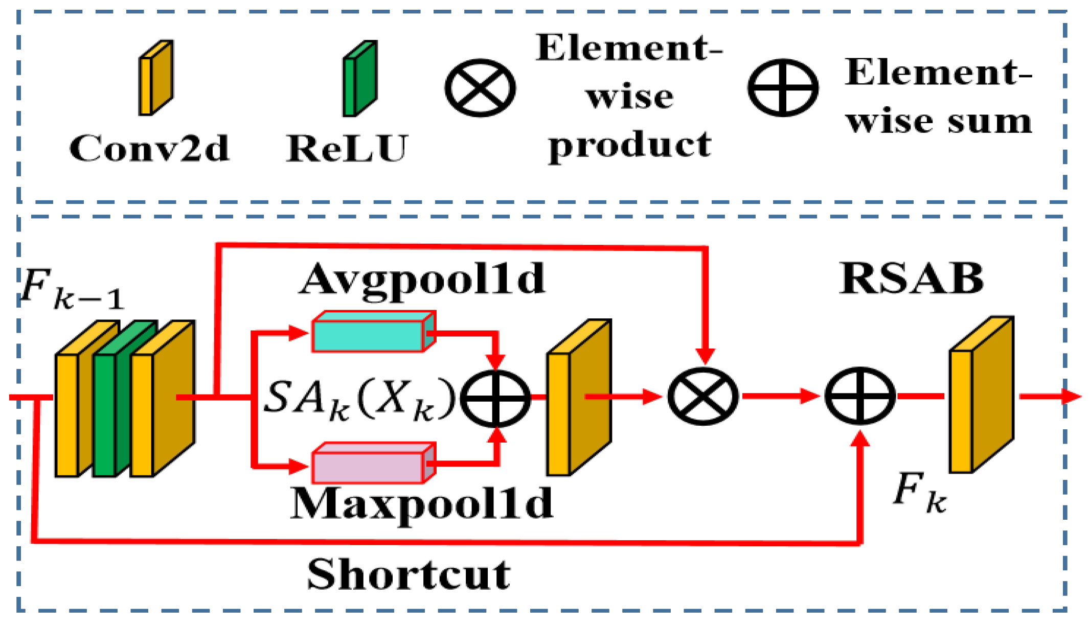
In this section, we design an RSAB component to extract the spatial information and refine the reconstructed texture. As exhibited in Figure 5, the RSAB employs a residual structure to represent the reconstructed maps. Suppose that the k-th output and input of the RSAB are $F_k$ and $F_{k-1}$. It can be calculated as follows:

$$F_k=F_{k-1}+{SA}_k\left(X_k\right)·X_k,$$

(8)

where $S{A}_k$ is the function of the spatial attention, and $X_k$ denotes the residual signal produced by two stacked convolution layers $(64\times 3\times 3\times 64)$ from $F_{k-1}$, as described in Formula (4). In contrast to the channel attention, the spatial attention concatenates them to generate an efficient feature descriptor for the spatial distribution. To reconstruct the remarkable texture, we compute the mean and max values of all the feature maps to weigh the residual signal $X_k$ acting as the spatial attention. The spatial attention is as follows:

$${SA}_k=Sigmoid\left({\omega }_{sa}\left[Avgpool1d\left(X_k\right);Maxpool1d\left(X_k\right)\right]\right),$$

(9)

where ${\omega }_{sa}$ is the coefficient of the Conv2d layer with a $1\times 7\times 7\times 2$ kernel, and $Avgpool1d(·)$ and $Maxpool1d(·)$ are the mean and max values of the residual signal $X_k$ over the different feature maps. The entire architecture is summarized in

Table 3. The main convolutional layers of the designed RSAB.

Convolutional Layer	Output Shape	Convolutional Layer	Output Shape
Conv2D_11_1	(H,W,64)	Conv2D_13_2	(H,W,64)
Conv2D_11_2	(H,W,64)	Conv2D_13_3	(H,W,1)
Conv2D_11_3	(H,W,1)	Conv2D_14_1	(H,W,64)
Conv2D_12_1	(H,W,64)	Conv2D_14_2	(H,W,64)
Conv2D_12_2	(H,W,64)	Conv2D_14_3	(H,W,1)
Conv2D_12_3	(H,W,1)	Conv2D_14_4	(H,W,64)
Conv2D_12_4	(H,W,64)	Conv2D_15	(H,W,64)
Conv2D_13_1	(H,W,64)	Conv2D_16	(H,W,C)

, and 16 Conv2D layers are employed to reconstruct the HR images. The first and second sets of three convolutional layers are designed to weigh and rescale the spatial features. These layers can encourage the network to focus on the prominent information. The seventh layer is adopted to fuse the residual and main signals from the previous layers. The next repeated layers are used to strengthen the network, and the last two layers are applied to reconstruct the HR images. We apply the spatial attention after the upsampling block to refine the spatial content.

3.5. Joint Loss Function

In this section, we refer to the joint loss function containing $L_1$ and MS-SSIM to estimate the parameters. Suppose that the i-th reference and reconstructed SR images are denoted as ${\mathbf{R}}_i\in {\mathcal{R}}^{H\times W\times C}$ and ${\mathbf{Y}}_i\in {\mathcal{R}}^{H\times W\times C}$. Then, the joint loss function $\mathcal{L}\left({\mathbf{R}}_i,{\mathbf{Y}}_i\right)$ can be calculated as follows:

$$\mathcal{L}\left({\mathbf{R}}_i,{\mathbf{Y}}_i\right)=L_1\left({\mathbf{R}}_i,{\mathbf{Y}}_i\right)+{\lambda }_1·L_{MS-SSIM}\left({\mathbf{R}}_i,{\mathbf{Y}}_i\right),$$

(10)

where $L_1({\mathbf{R}}_i,{\mathbf{Y}}_i)$ and $L_{MS-SSIM}({\mathbf{R}}_i,{\mathbf{Y}}_i)$ are the $L_1$ and MS-SSIM loss functions, and ${\lambda }_1$ is a weight to adjust the values of two loss functions to the same range of magnitude. Here, $L_1({\mathbf{R}}_i,{\mathbf{Y}}_i)$ can be formulated as:

$$L_1\left({\mathbf{R}}_i,{\mathbf{Y}}_i\right)=\frac{1}{H\times W\times C}·{\displaystyle \sum _{c=1}^C}{\displaystyle \sum _{h=1}^H}{\displaystyle \sum _{w=1}^W}\left|{\mathbf{R}}_i\left(h,w,c\right)-{\mathbf{Y}}_i\left(h,w,c\right)\right|,$$

(11)

where H, W, and C are the height, width, and channel number of the remote sensing images. $L_{MS-SSIM}({\mathbf{R}}_i,{\mathbf{Y}}_i)$ is computed as follows:

$$L_{MS-SSIM}\left({\mathbf{R}}_i,{\mathbf{Y}}_i\right)=1-{\displaystyle \sum _{n=1}^N}{\gamma }_n·SSIM\left({\mathbf{R}}_{i,n},{\mathbf{Y}}_{i,n}\right),$$

(12)

where $N=5$ is the scale number, ${\displaystyle \sum _{n=1}^N}{\gamma }_n=1$ is weight values, and $R_{i,n}$ and $Y_{i,n}$ are the downsampling images with a scale factor of $2^n$. As recommended by the former work [50], the parameters are ${\gamma }_1=0.0448$, ${\gamma }_2=0.2856$, ${\gamma }_3=0.3001$, ${\gamma }_4=0.2363$, and ${\gamma }_5=0.1333$, respectively.

Generally, compared with the traditional $L_2$ loss function, $L_1$ is insensitive to outliers and prevents exploding gradients in some cases. Moreover, the MS-SSIM loss function forces the network to acquire the HR images with a more detailed texture than using only the $L_1$ loss function. Therefore, we employ this joint function to constrain the whole framework.

4. Results

In this section, we first clarify the public SR datasets, evaluation metrics, and training settings. Then, we compare the performance of our HSRN with the state-of-the-art SR algorithms, including Bicubic [12], ESPCN [26], RDN [28], RCAN [25,26], CSCLN [31], ENLCN [32], 3D-FCNN [33], HSENet [36], and TransENet [37] for multi-channel remote sensing images. We report the mean peak signal-to-noise ratio (PSNR), mean structural similarity (SSIM) [51], and mean spectral angle mapper (SAM) [52] indices on the different datasets. Moreover, we further present the visual comparison of the images reconstructed by the SR models, following each experimental dataset.

4.1. Experimental Datasets

To prove the performance of our models with multi-channel remote sensing images from different sources and resolutions, three public datasets were introduced in our experiment with a brief review in terms of band range and image resolution, as shown in

Table 4. A brief review of three public datasets.

Dataset	Band Number	Band Range	Spatial Resolution
AVIRIS	224	From 350 nm to 2500 nm	16 m
SEN12MS-CR	13	From 400 nm to 2500 nm	10 m
WHU Building	3	Red, green, and blue bands	0.2 m

. These datasets have decreasing channel numbers for proving the SR performance. The original images were considered HR images, and we downsampled each image as a LR image.

Hyperspectral AVIRIS dataset [53]: these images were acquired by the airborne visible/infrared imaging spectrometer (AVIRIS) over the seaside area in Salinas, with a spatial resolution of 16 m. It can be downloaded from NASA’s website (http://aviris.jpl.nasa.gov/data/get_aviris_data.html, accessed on 18 November 2016). It contains 224 spectral bands ranging from 350 nm to 2500 nm. The images are reflectance products (the proportion of the radiation striking a surface to the radiation reflected off of it), and pixel values are in the range of $[0,1]$. Both the training and test datasets had 241 hyperspectral images, and each picture consists of $256\times 256$ pixels.

Multispectral SEN12MS-CR dataset [54]: these images were chosen from the Sentinel-2 satellite, with different types of ground surfaces included, such as farmland, rivers, and urban and mountain areas. The acquired images have 13 channels, and the spectral range is from 400 nm to 2500 nm. The images include radiance data and pixel values were normalized to $[0,1]$. The images were resampled and have an unified spatial resolution of 10 m, and the cropped images are composed of $256\times 256$ pixels. To save experimental time, we chose partial data (file number is “summer_s2_147”) from the SEN12MS-CR dataset to run the SR model. Both the training and test datasets had 297 images.

Three-channel WHU Building dataset [55]: the images consist in a large number of independent buildings extracted from aerial images covering Christchurch, New Zealand. The dataset contains rural, residential, cultural, and industrial areas, and each image has three channels, including red, green, and blue (RGB) bands. The size of these images is $512\times 512$ and the spatial resolution is 0.2 m. The values were normalized to $[0,1]$. The training and test datasets had 1260 and 690 images.

4.2. Evaluation Metrics and Parameter Setting

4.2.1. Evaluation Metrics

Three evaluation metrics, i.e., PSNR, SSIM, and SAM, were employed in our experiment to quantitatively assess the SR models. The PSNR evaluates the mean peak signal-to-noise ratio between the i-th reference image $R_i$ and the reconstructed HR image $Y_i$. The definition is as follows:

$$PSNR={\displaystyle \sum _{i=1}^N}10{log}_{10}\frac{1}{{\left(R_i-Y_i\right)}^2},$$

(13)

A larger PSNR value indicates a higher quality of the reconstructed HR images.

The SSIM measures the mean structural similarity between the i-th reference image $R_i$ and the reconstructed HR images $Y_i$. The definition is as follows:

$$SSIM={\displaystyle \sum _{i=1}^N}\left(\frac{\left(2{\mu }_{R_i}{\mu }_{Y_i}+C_1\right)·\left(2{\sigma }_{R_i{Y}_i}+C_2\right)}{\left({\mu }_{R_i}^2+{\mu }_{Y_i}^2+C_1\right)·\left({\sigma }_{R_i}^2+{\sigma }_{Y_i}^2+C_2\right)}\right),$$

(14)

where ${\mu }_{R_i}$ and ${\mu }_{Y_i}$ are the mean value of the i-th reference image $R_i$ and the reconstructed HR image $Y_i$, ${\sigma }_{R_i}$ and ${\sigma }_{Y_i}$ are the corresponding standard values, ${\sigma }_{R_i{Y}_i}$ is the covariance between the reference image $R_i$ and the reconstructed HR images $Y_i$, and $C_2={\left(3·C_1\right)}^2={0.03}^2$ (recommended by the former study [51]). The value of SSIM is in the range of 0–1, and the image quality increases as the SSIM increases.

The SAM calculates the mean spectral angle mapper between the reference images $R_i$ and the reconstructed HR images $Y_i$. The definition is as follows:

$$SAM=\frac{180}{\pi }·{\displaystyle \sum _{i=1}^N}arccos\left(\frac{{\sum }_{j=1}^{WH}{r}_i\left(j\right)y_i\left(j\right)}{{\left({\sum }_{j=1}^{WH}{r}_i^2\left(j\right)\right)}^{1/2}·{\left({\sum }_{j=1}^{WH}{y}_i^2\left(j\right)\right)}^{1/2}}\right),$$

(15)

where W and H are the width and height of the reference image $R_i$ and the reconstructed HR image $Y_i$, and $r_i$ and $y_i$ are the spectral curves of the reference image $R_i$ and the reconstructed HR image $Y_i$, respectively. The SAM values range from 0° to 90°. The SAM values near zero indicate high spectral quality.

4.2.2. Parameters Setting

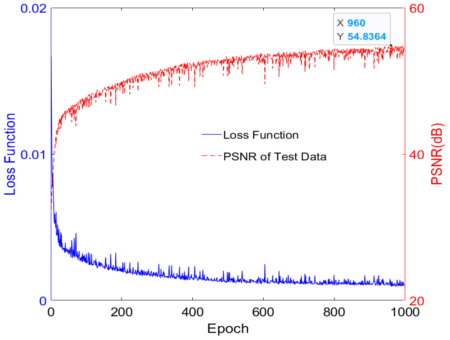
For the fairness of the experiment, all of the SR methods were trained on three remote sensing datasets separately and adopted the same hyperparameters to construct the SR models. We adopted the adaptive moment estimation (ADAM) to optimize the network, and the size of the label tensors was $256\times 256$. We saved and selected the best model after running them for 1000 epochs. We set both the training and test batch sizes to 2, and the learning rate to $1\times {10}^{-4}$. All the compared models were the original codes downloaded from the corresponding reference papers. A detailed running time will be presented in the following subsection. After setting these parameters, the PSNR of our HSRN increased, accompanied by a decreasing loss function, as shown in Figure 6. The stability and convergence of the loss function proves its behavior with good parametrics.

4.3. SR Performance

4.3.1. AVIRIS Dataset

We first tested the SR algorithms on the AVIRIS dataset, which has 224 spectral channels, and the quantitative results are reported in

Table 5. Quantitative results of super-resolution models on the AVIRIS dataset. Indices with bold types for all tables represent the best performance achieved in the same row.

Scale		Bicubic	ESPCN	RDN	RCAN	CSNLN	ENLCN	3D-FCNN	HSENet	TransENet	Ours
×2	PSNR	43.7178	41.9711	45.6773	46.0382	45.3586	45.1305	44.5548	45.8904	45.9450	46.4883
	SSIM	0.9738	0.9685	0.9838	0.9840	0.9827	0.9819	0.9782	0.9844	0.9849	0.9849
	SAM	0.1383	1.9282	0.4562	0.4723	0.4245	0.4446	0.1102	0.4611	0.6681	0.4680
×4	PSNR	39.2244	38.3873	40.6197	41.0866	40.7598	40.3743	39.3862	40.7832	41.4172	41.6898
	SSIM	0.9373	0.9250	0.9538	0.9579	0.9547	0.9518	0.9389	0.9551	0.9610	0.9615
	SAM	0.9679	1.8873	0.9505	0.9410	1.0092	0.9933	0.9592	1.0030	1.0487	0.9335
×8	PSNR	36.1034	33.7565	37.3726	38.0435	37.5841	37.5112	36.4650	37.2758	38.0328	38.2285
	SSIM	0.9036	0.8321	0.9200	0.9295	0.9232	0.9220	0.9062	0.9182	0.9286	0.9304
	SAM	2.8432	3.0559	2.2265	2.0168	2.2273	2.2132	2.5287	2.3122	2.1520	2.1058

. Indices with bold types represent the best performance achieved in the same row, where three upsampling factors containing ×2, ×4, and ×8 are calculated and exhibited. In contrast, our HSRN delivered better PSNR and SSIM scores compared to the other algorithms for all scale factors. In particular, the PSNR of our model was greater than that of the state-of-the-art TransENet method by 0.5433 dB, 0.2726 dB, and 0.1957 dB for the ×2, ×4, and ×8 scale factor. It is worth noting that our model achieved an average performance in the SAM index. This result also demonstrated that our model sacrificed spectral accuracy to enhance the spatial resolution. The reconstructed spectral curves are probably affected by the low signal-to-noise ratio (SNR) channels, which were preserved in the comparison.

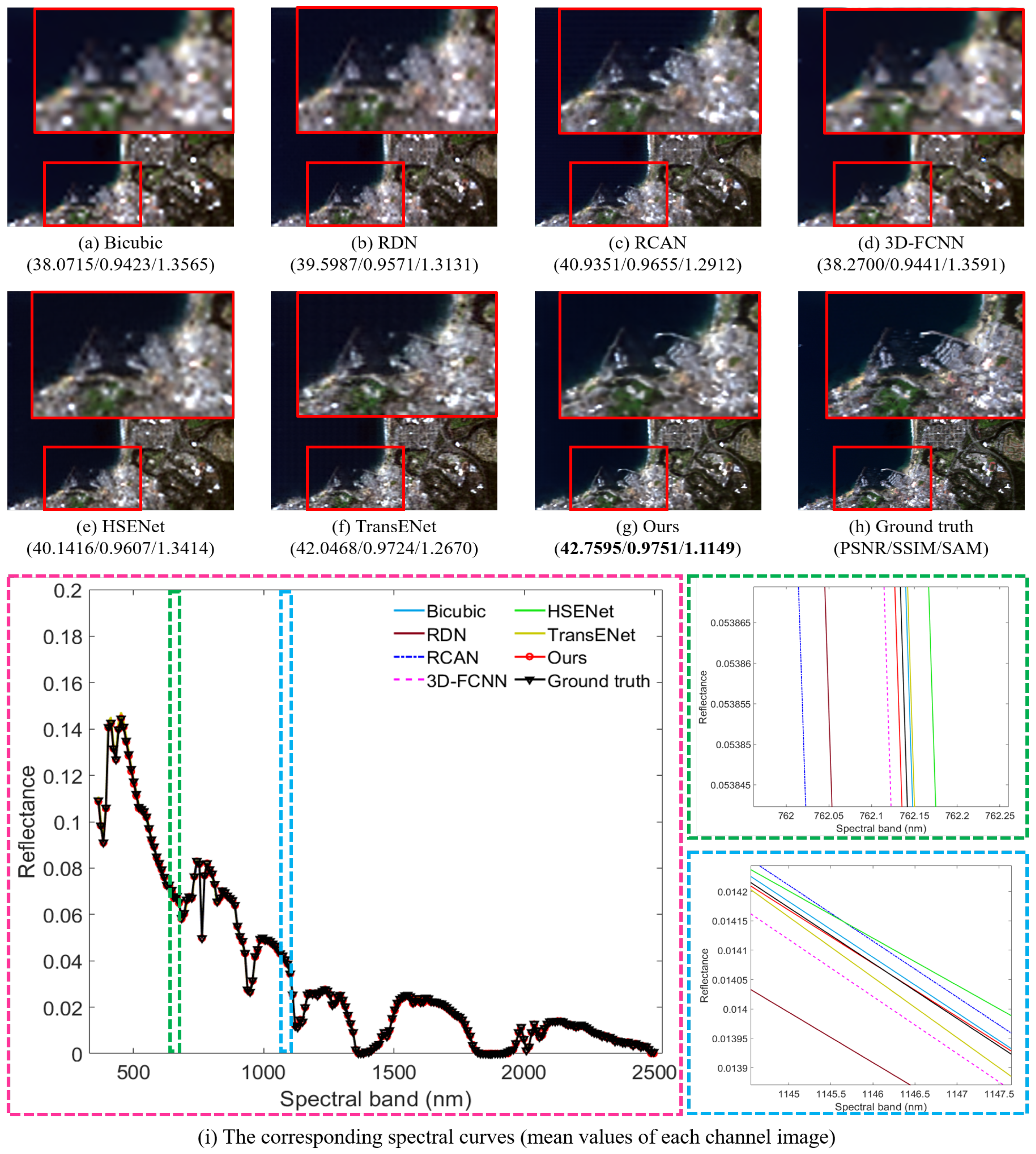
The qualitative comparisons are presented in Figure 7, where we recorded the sea and urban areas from the AVIRIS dataset. Figure 7a–g are the SR results (×4) of the Bicubic, RDN, RCAN, 3D-FCNN, HSENet, TransENet, and the proposed model, and Figure 7h,i are the ground truth and corresponding spectral curve. As shown in Figure 7h, the sea area contains a lot of port buildings (highlighted by red rectangles) standing in sharp contrast to the seawater on the left. The SR results in the Bicubic, RDN, and 3D-FCNN suffer from a blurring effect. The reconstructed images of the RCAN, HSRNet, and TransENet reveal that the boundaries of the different architectures tend to mix with each other. Our model achieved the best visual effect compared with the other SR models, and recovered the rich texture of the port facilities. The evaluation indices of our HSRN were 42.7595 dB, 0.9751, and 1.1149°, which is better than those of the other methods. More importantly, as shown in Figure 7i, our recovered spectra (red circle) were most similar to those of the ground truth (black triangle), proving the SR’s superior performance.

To demonstrate the SR’s performance on different scenes, we tested the SR models on mountain areas, as shown in Figure 8. Figure 8a–g show the SR results (×4) of the Bicubic, RDN, RCAN, 3D-FCNN, HSENet, TransENet, and the proposed model, and Figure 8h,i are the ground truth and corresponding spectral curve. Again, our model outperformed the other SR algorithms, and alleviated the blurring artifacts. Our HSRN recovered more details in the mountain chain, as exhibited in Figure 8g. The reconstructed texture of our model highlighted in red rectangles was clearer than that of the state-of-the-art models. Meanwhile, the reconstructed spectral data of our SR model were more similar to those of the ground truth than those of the compared methods, indicating that our algorithm enhances the resolution of multi-channel images quite effectively at the expense of weak spectral distortion (Figure 8i).

4.3.2. SEN12MS-CR Dataset

Next, we tested the SR models on the SEN12MS-CR dataset, which contains 13 channels, as listed in

Table 6. Quantitative results of super-resolution models on the SEN12MS-CR dataset.

Scale		Bicubic	ESPCN	RDN	RCAN	CSNLN	ENLCN	3D-FCNN	HSENet	TransENet	Ours
×2	PSNR	45.6728	48.4261	52.1085	53.9716	51.2913	49.6070	48.5111	54.0833	53.6462	54.8343
	SSIM	0.9896	0.9933	0.9973	0.9982	0.9968	0.9955	0.9936	0.9982	0.9980	0.9985
	SAM	0.2009	0.2941	0.1975	0.2002	0.2276	0.2031	0.2361	0.1895	0.2615	0.2202
×4	PSNR	39.3311	40.9415	42.3691	43.8431	43.3067	41.4983	40.2574	43.7074	45.3179	45.5625
	SSIM	0.9601	0.9688	0.9769	0.9827	0.9805	0.9728	0.9639	0.9825	0.9879	0.9882
	SAM	0.5553	0.5311	0.3934	0.3700	0.4113	0.4250	0.5154	0.3987	0.6190	0.3806
×8	PSNR	33.6025	35.1888	36.2570	38.5665	37.9443	35.9386	34.4387	37.2628	40.3338	41.0994
	SSIM	0.9074	0.9221	0.9341	0.9546	0.9502	0.9314	0.9125	0.9436	0.9678	0.9738
	SAM	1.9642	1.4279	1.2314	0.9549	1.0551	1.2219	1.5838	1.1569	0.8413	0.7764

. When compared with the other methods, our model outperformed the other algorithms with respect to all the spatial evaluation indices (PSNR and SSIM) for all scaling factors. The relative gap between the HSRN (Our model) and the other models, which increases with the upsampling factors, deserves particular attention. Especially for the ×8 scale factor, our model achieved an outstanding performance, and the values of the PSNR, SSIM, and SAM are 41.0994 dB, 0.9738, and 0.7764°. The SAM values of our model are at top of the list, verifying the spectral fidelity of our reconstructed HR data. It turns out that our model exploits the spectral information to enhance the spatial resolution.

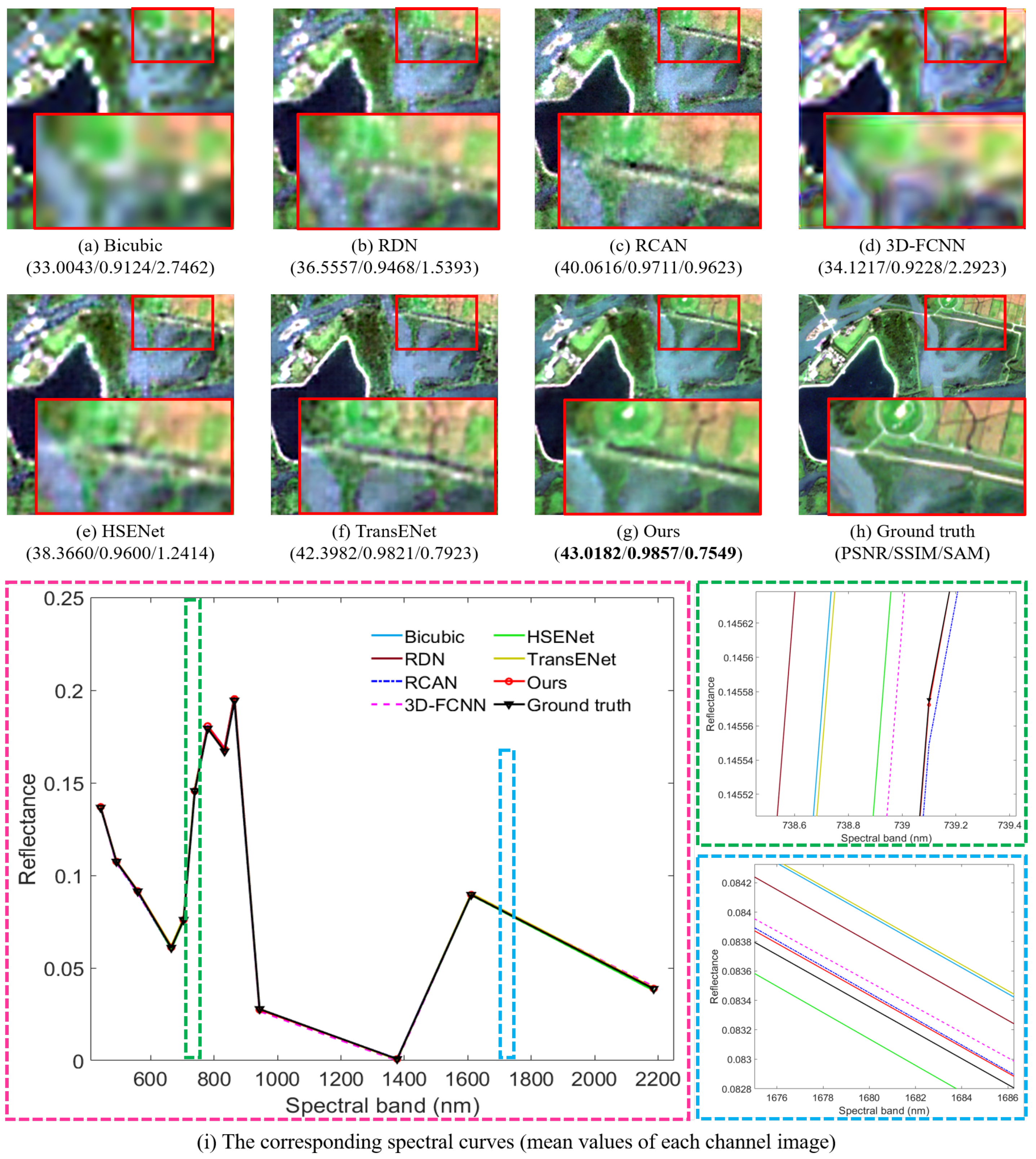
The visual comparisons of the SR model on the river and urban areas are illustrated in Figure 9 and Figure 10, respectively. Figure 9a–g are the SR results (×8) of the Bicubic, RDN, RCAN, 3D-FCNN, HSENet, TransENet, and the proposed model, and Figure 9h,i are the ground truth and corresponding spectral curve. The SR maps of the Bicubic and 3D-FCNN suffer from heavy blurring artifacts, and the remaining SR maps are slightly contaminated by noise data, failing to recover more details. From Figure 9h, we observe that our model achieved a better visual performance (highlighted by the red rectangle), containing fewer artifacts and a more detailed texture, which is consistent with the evaluation metrics. Moreover, the reconstructed spectral curve of the HSRN (red circles) is closer to the ground truth (black triangle) than that of the other algorithms.

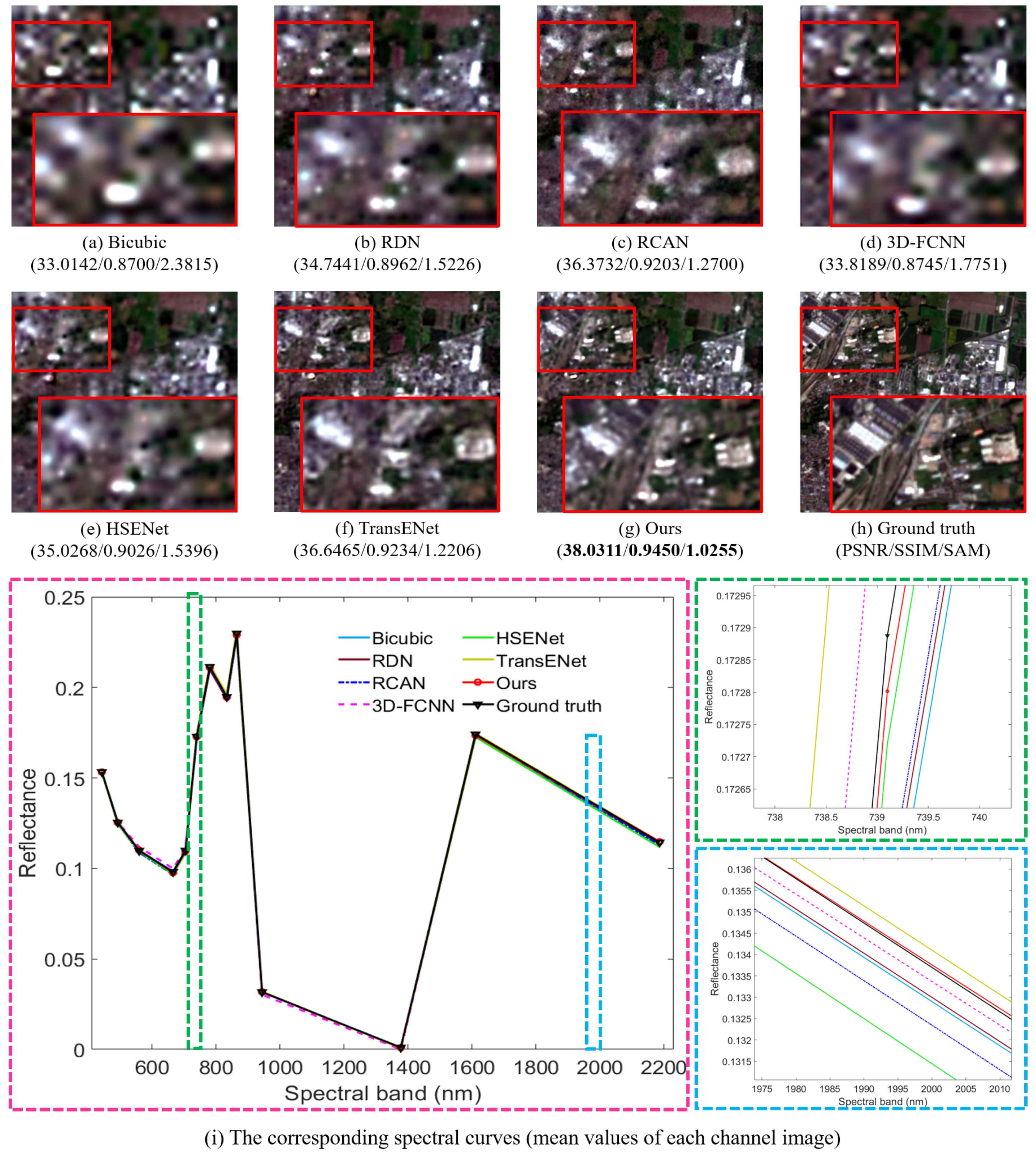
To prove the model’s scene adaptivity, Figure 10 exhibits the SR results of the urban area, which consist in detailed texture. Figure 10a–g are the SR results (×8) of the Bicubic, RDN, RCAN, 3D-FCNN, HSENet, TransENet, and the proposed model, respectively, and Figure 10h,i are the ground truth and corresponding spectral curve, respectively. The recovered HR images and spectral curves of our HSRN are more faithful to the ground truth. Nevertheless, all the compared approaches were affected by different degrees of blur (highlighted by red rectangles). Such obvious comparisons demonstrate that our model can extract sophisticated features and effectively improve the resolution of multi-channel images.

4.3.3. WHU Building Dataset

To demonstrate the SR effectiveness for remote sensing images, we first compared our network with the hand-crafted and CNN-based models on the WHU Building dataset consisting of only RGB channels. The quantitative results for scale factors ×2, ×4, and ×8 are presented in

Table 7. Quantitative results of super-resolution models in the WHU Building dataset.

Scale		Bicubic	ESPCN	RDN	RCAN	CSNLN	ENLCN	3D-FCNN	HSENet	TransENet	Ours
×2	PSNR	23.8249	26.3325	27.0202	27.0111	26.9092	25.8780	26.0320	27.0019	26.6260	27.0671
	SSIM	0.6891	0.8084	0.8230	0.8235	0.8211	0.7968	0.7975	0.8228	0.8140	0.8282
	SAM	0.1739	0.2493	0.1702	0.1654	0.1973	0.1707	0.1977	0.1638	0.1999	0.2068
×4	PSNR	21.6610	22.9743	23.3805	23.3446	23.2715	22.7953	22.7498	23.3512	23.1586	23.3269
	SSIM	0.5124	0.6107	0.6347	0.6337	0.6317	0.6005	0.5920	0.6321	0.6241	0.6379
	SAM	0.2860	0.2730	0.2127	0.2318	0.2879	0.2244	0.2903	0.2189	0.3381	0.3078
×8	PSNR	20.0802	20.9555	21.1534	21.1195	21.0724	20.9007	20.7813	21.0925	21.0997	20.8123
	SSIM	0.4043	0.4597	0.4772	0.4752	0.4779	0.4533	0.4456	0.4706	0.4787	0.4768
	SAM	0.6160	0.5683	0.3937	0.4449	0.5800	0.3858	0.5382	0.4848	0.6052	0.5883

. The PSNR and SSIM of our model are at top of the list, proving SR’s applicability. Specifically, our HSRN achieved the best PSNR and SSIM of all the models when the scaling factor was ×2×2. It is worth noting that the SSIM of our model was higher than that of the other methods for almost all scaling factors, due to the joint loss function we applied. The SAM of our model is not outstanding, perhaps because it is tricky for the 3D hybrid module to extract the spectral information from images only with three channels. Our model may sacrifice the spectral accuracy to improve the resolution of the reconstruction images. Furthermore, the SAM measures the spectral similarity between the reconstructed and original images, so the SAM indice is more suitable for multispectral or hyperspectral data, but the images of the WHU Building dataset are RGB images, which only have three channels. We also present the visual reconstruction images from the WHU Building dataset, as shown in Figure 11. Figure 11a–g are the SR results (×4) of the Bicubic, RDN, RCAN, 3D-FCNN, HSENet, TransENet, and the proposed model, and Figure 11h,i are the ground truth and corresponding spectral curve. Our model obtains the best reconstruction performance compared to the state-of-the-art SR models. The corresponding PSNR and SSIM of our algorithm are 23.8611 dB and 0.5763, which are slightly higher than the compared models, demonstrating that our method is applicable for only-three-channel remote sensing images. The reconstructed car highlighted by red rectangles in Figure 11g is most similar to those of the ground truth, proving the SR’s superior performance. The reconstructed spectral curves look similar in Figure 11i on the left. Our spectral curve is reconstructed with poor appearance in the right corner of the Figure 11i. This phenomenon proves that our model applies the spectral information to enhance the remote sensing images.

In summary, one notable advantage of our method lies in its strong generalization ability. Our model is insensitive to the number of bands and content variations, making it suitable for common super-resolution tasks in hyperspectral, multispectral, and three-band remote sensing images. Additionally, our model demonstrates a strong representational capability, resulting in higher accuracy when reconstructing super-resolved images compared to state-of-the-art algorithms. However, a drawback of our model is that the fidelity of reconstructing spectra is average, as the emphasis was placed on enhancing the super-resolution effect at the expense of the spectral reconstruction capacity.

5. Discussion

In this section, we analyze the key factors which affect the SR’s performance and need to be considered in practical applications.

5.1. Loss Function Parameter

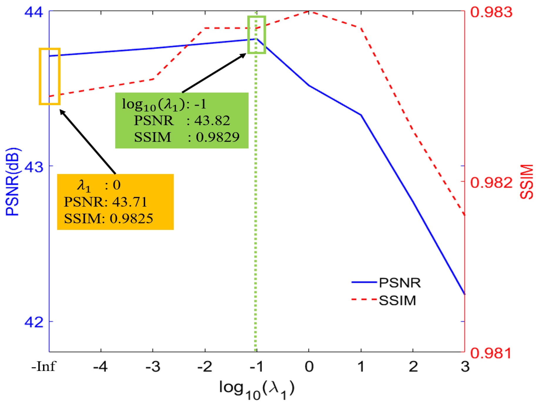
To select the best weight for the loss function, we tested our model with the distinct parameter ${\lambda }_1$ on the SEN12MS-CR dataset. We selected the best result over 200 epochs (to save running time) with a scaling factor of ×4. As exhibited in Figure 12, the line graph illustrates changes in the evaluated metrics along with the variation in parameter ${\lambda }_1$. The PSNR rises slightly from ${\lambda }_1=0$ to ${\lambda }_1=0.1$, before falling sharply at ${\lambda }_1=1$. Meanwhile, the SSIM gradually increases, peaking at ${\lambda }_1=1$, and achieves a rapid decline at ${\lambda }_1=10$. This result demonstrates that our model is sensitive to the parameter ${\lambda }_1$. We set ${\lambda }_1=0.1$, avoiding a significant decline in PSNR.

5.2. Ablation Investigation

To verify the effectiveness of each component, we tested the SR’s performance by removing the individual block from the HSRN. The quantitative consequences are shown in Figure 13 and

Table 8. Quantitative evaluation of the ablation experiments.

Ablation	PSNR	SSIM
w/o all three modules	41.2360	0.9715
w/o RCAB and RSAB	42.6327	0.9782
w/o 3D and RSAB	43.9234	0.9832
w/o 3D and RCAB	43.5476	0.9816
w/o RSAB	44.4369	0.9849
w/o RCAB	44.4971	0.9851
w/o 3D	45.3522	0.9869
Ours	45.5625	0.9882

, showing that all the networks gradually converge. The basic SR model (without 3D, RCAB, and RSAB modules) obtained the worst reconstruction result, and the PSNR and SSIM were 41.2360 dB and 0.9715. The employment of the 3D, RCAB, and RSAB modules increased the PSNR by 3.39%, 6.52%, and 5.61%, respectively. This proves that all three modules are beneficial to the SR task, and that the RCAB is more effective than the others. The 3D module extracts the spectral-spatial information from the multi-channel remote sensing images and gains 1.3967 dB more than the basic SR models. The attention structure of the RCAB and RSAB strength’s spectral and spatial features achieved 2.6874 dB and 2.3116 dB more than the basic SR models. Moreover, the combination of these modules is more important than a single module for the RS model. The attention structure containing the RCAN and RSAB outperformed the other pairs. The best performance was achieved by our HSRN, proving the validity of the 3D, RCAB, and RSAB modules.

5.3. Training and Testing Times

Here, we present the training and testing times for the end-to-end model. All the tests were performed on a workstation with two Intel Xeon(R) Gold 5128 central processing units, 128 GB memory, and four NVIDIA GeForce RTX 3090 GPUs. The operating system was Windows 10. In

Table 9. Training and testing time on the SEN12MS-CR dataset with an upsampling scale of ×2. The unit of time is seconds.

Models	Training Time	Testing Time
ESPCN	12.3096	12.06227
RDN	12.8103	12.4258
RCAN	13.8602	12.7183
CSNLN	45.1342	21.5814
ENLCN	25.4723	24.4237
3D-FCNN	24.9178	17.1695
HSENet	33.5243	17.9910
TransENet	27.1521	17.2124
Ours	26.2231	15.9818

, we can see that the proposed method had little advantage in computational time consumed due to its complex construction. Our model only had a faster testing speed than the CSNLN, 3D-FCNN, HSENet, and TransENet. Future work will focus on model simplification.

6. Conclusions

In this paper, we proposed a hybrid SR network (HSRN) for multi-channel remote sensing images. Specifically, the hybrid 3D–2D module allows the HSRN to extract the spatial-spectral information from the LR images. Then, we designed an attention structure consisting of channel and spatial attention, and adopted it to weigh and rescale the features. Furthermore, we applied a joint loss function to constrain the HSRN to reconstruct HR remote sensing images. Most evaluations of three public datasets proved that our model not only gains higher PSNR and SSIM values, but also generates clearer visualization SR outputs than the compared models. The spectral curves of our reconstructed images maintained stability and our model utilized spectral information to improve the SR performance. Extensive experiments demonstrated the effectiveness of our HSRN. In future work, we will optimize the HSRN and improve its operation efficiency. We will also further explore the feasibility of applying our method to achieve super-resolution for synthetic aperture radar (SAR) images.

References

1. Zhang, B.; Liu, Y.; Zhang, W.; Gao, L.; Li, J.; Wang, J.; Li, X. Analysis of the Proportion of Surface Reflected Radiance in Mid-Infrared Absorption Bands. IEEE J. Sel. Top. Appl. Earth Obs. Remote Sens. 2014, 7, 2639–2646. [Google Scholar] [CrossRef]
2. Zhou, S.; Wang, W.; Gao, C. Learning-Free Hyperspectral Anomaly Detection with Unpredictive Frequency Residual Priors. IEEE J. Sel. Top. Appl. Earth Obs. Remote Sens. 2022, 15, 6294–6305. [Google Scholar] [CrossRef]
3. Li, Z.; Zhao, B.; Wang, W. An Efficient Spectral Feature Extraction Framework for Hyperspectral Images. Remote Sens. 2020, 12, 3967. [Google Scholar] [CrossRef]
4. Hong, D.; Gao, L.; Yao, J.; Zhang, B.; Plaza, A.; Chanussot, J. Graph Convolutional Networks for Hyperspectral Image Classification. IEEE Trans. Geosci. Remote Sens. 2021, 59, 5966–5978. [Google Scholar] [CrossRef]
5. Dian, R.; Li, S.; Fang, L.; Bioucas-Dias, J. Hyperspectral Image Super-Resolution via Local Low-Rank and Sparse Representations. In Proceedings of the IEEE International Geoscience and Remote Sensing Symposium, Valencia, Spain, 22–27 July 2018; pp. 4003–4006. [Google Scholar]
6. Liu, X.; Liu, Q.; Wang, Y. Remote sensing image fusion based on two-stream fusion network. Inform. Fusion 2020, 55, 1–15. [Google Scholar] [CrossRef] [Green Version]
7. Huang, L.; Hu, Z.; Luo, X.; Zhang, Q.; Wang, J.; Wu, G. Stepwise Fusion of Hyperspectral, Multispectral and Panchromatic Images with Spectral Grouping Strategy: A Comparative Study Using GF5 and GF1 Images. Remote Sens. 2022, 14, 1021. [Google Scholar] [CrossRef]
8. UI Hoque, M.R.; Burks, R.; Kwan, C.; Li, J. Deep Learning for Remote Sensing Image Super-Resolution. In Proceedings of the 2019 IEEE 10th Annual Ubiquitous Computing, Electronics and Mobile Communication Conference (UEMCON), New York, NY, USA, 10–12 October 2019; pp. 0286–0292. [Google Scholar]
9. Han, Y.; Wang, H.; Zhang, Z.; Wang, W. Boundary-aware vehicle tracking upon UAV. Electron. Lett. 2020, 56, 873–876. [Google Scholar] [CrossRef]
10. Ayhan, B.; Kwan, C. Mastcam Image Resolution Enhancement with Application to Disparity Map Generation for Stereo Images with Different Resolutions. Sensors 2019, 19, 3526. [Google Scholar] [CrossRef] [Green Version]
11. Wang, L.; Li, D.; Tian, L.; Shan, Y. Efficient Image Super-Resolution with Collapsible Linear Blocks. In Proceedings of the 2022 IEEE/CVF Conference on Computer Vision and Pattern Recognition Workshops, New Orleans, LA, USA, 19–20 June 2022; pp. 816–822. [Google Scholar]
12. Keys, R. Cubic convolution interpolation for digital image processing. IEEE Trans. Acoust. Speech Signal Process. 1981, 29, 1153–1160. [Google Scholar] [CrossRef] [Green Version]
13. Ma, J.; Chan, J.C.W.; Canters, F. Robust locally weighted regression for superresolution enhancement of multi-angle remote sensing imagery. IEEE J. Sel. Top. Appl. Earth Observ. Remote Sens. 2014, 7, 1357–1371. [Google Scholar] [CrossRef]
14. Schulter, S.; Leistner, C.; Bischof, H. Fast and accurate image upscaling with super-resolution forests. In Proceedings of the 2015 IEEE Conference on Computer Vision and Pattern Recognition, Boston, MA, USA, 7–12 June 2015; pp. 3791–3799. [Google Scholar]
15. Timofte, R.; Rothe, R.; Gool, L.V. Seven Ways to Improve Example-Based Single Image Super Resolution. In Proceedings of the 2016 IEEE Conference on Computer Vision and Pattern Recognition, Las Vegas, NV, USA, 26–30 June 2016; pp. 1865–1873. [Google Scholar]
16. Yang, J.; Wright, J.; Huang, T.S.; Ma, Y. Image super-resolution via sparse representation. IEEE Trans. Image Process. 2010, 19, 2861–2873. [Google Scholar] [CrossRef] [PubMed]
17. Peleg, T.; Elad, M. A statistical prediction model based on sparse representations for single image super-resolution. IEEE Trans. Image Process. 2014, 23, 2569–2582. [Google Scholar] [CrossRef]
18. Hou, B.; Zhou, K.; Jiao, L. Adaptive Super-Resolution for Remote Sensing Images Based on Sparse Representation with Global Joint Dictionary Model. IEEE Trans. Geosci. Remote Sens. 2018, 56, 2312–2327. [Google Scholar] [CrossRef]
19. Shao, Z.; Wang, L.; Wang, Z.; Deng, J. Remote Sensing Image Super-Resolution Using Sparse Representation and Coupled Sparse Autoencoder. IEEE J. Sel. Top. Appl. Earth Observ. Remote Sens. 2019, 12, 2663–2674. [Google Scholar] [CrossRef]
20. Zhang, L.; Yang, M.; Feng, X. Sparse representation or collaborative representation: Which helps face recognition? In Proceedings of the 2011 IEEE International Conference on Computer Vision, Colorado Springs, CO, USA, 20–25 June 2011; pp. 471–478. [Google Scholar]
21. Sun, Y.; Zhang, Z.; Jiang, W.; Liu, G.; Yan, S. Robust discriminative projective dictionary pair learning by adaptive representations. In Proceedings of the International Conference on Pattern Recognition, Beijing, China, 20–24 August 2018; pp. 621–626. [Google Scholar]
22. Huan, H.; Li, P.; Zou, N.; Wang, C.; Xie, Y.; Xie, Y.; Xu, D. End-to-End Super-Resolution for Remote-Sensing Images Using an Improved Multi-Scale Residual Network. Remote Sens. 2021, 13, 666. [Google Scholar] [CrossRef]
23. Patil, V.H.; Bormane, D.S.; Pawar, V.S. Super Resolution Using Neural Network. In Proceedings of the 2008 Second Asia International Conference on Modelling and Simulation, Los Alamitos, CA, USA, 13–15 May 2008; pp. 492–496. [Google Scholar]
24. Su, Y.-F.; Foody, G.M.; Muad, A.M.; Cheng, K.-S. Combining Hopfield Neural Network and Contouring Methods to Enhance Super-Resolution Mapping. IEEE J. Sel. Top. Appl. Earth Observ. Remote Sens. 2012, 5, 1403–1417. [Google Scholar] [CrossRef]
25. Dong, C.; Loy, C.C.; He, K.; Tang, X. Learning a deep convolutional network for image super-resolution. In Proceedings of the European Conference on Computer Vision, Zurich, Switzerland, 6–12 September 2014; pp. 184–199. [Google Scholar]
26. Shi, W.; Caballero, J.; Huszár, F.; Wang, Z. Real-time single image and video super-resolution using an efficient sub-pixel convolutional neural network. In Proceedings of the 2016 IEEE Conference on Computer Vision and Pattern Recognition, Las Vegas, NV, USA, 26–30 June 2016; pp. 1874–1883. [Google Scholar]
27. Kim, J.; Lee, J.K.; Lee, K.M. Accurate Image Super-Resolution Using Very Deep Convolutional Networks. In Proceedings of the 2016 IEEE Conference on Computer Vision and Pattern Recognition, Las Vegas, NV, USA, 26–30 June 2016; pp. 1646–1654. [Google Scholar]
28. Zhang, Y.; Tian, Y.; Kong, Y.; Zhong, B.; Fu, Y. Residual Dense Network for Image Super-Resolution. In Proceedings of the 2018 IEEE/CVF Conference on Computer Vision and Pattern Recognition, Salt Lake City, UT, USA, 18–22 June 2018; pp. 2472–2481. [Google Scholar]
29. Zhang, Y.; Li, K.; Li, K.; Wang, L.; Zhong, B.; Fu, Y. Image super-resolution using very deep residual channel attention networks. In Proceedings of the European Conference on Computer Vision, Munich, Germany, 8–14 September 2018; pp. 294–310. [Google Scholar]
30. Basak, H.; Kundu, R.; Agarwal, A.; Giri, S. Single Image Super-Resolution using Residual Channel Attention Network. In Proceedings of the 2020 IEEE 15th International Conference on Industrial and Information Systems, Rupnagar, India, 26–28 November 2020; pp. 219–224. [Google Scholar]
31. Mei, Y.; Fan, Y.; Zhou, Y.; Huang, L.; Huang, T.S.; Shi, H. Image Super-Resolution With Cross-Scale Non-Local Attention and Exhaustive Self-Exemplars Mining. In Proceedings of the 2020 IEEE/CVF Conference on Computer Vision and Pattern Recognition, Seattle, WA, USA, 14–19 June 2020; pp. 5689–5698. [Google Scholar]
32. Xia, B.; Hang, Y.; Tian, Y.; Yang, W.; Liao, Q.; Zhou, J. Efficient Non-Local Contrastive Attention for Image Super-Resolution. In Proceedings of the 2022 IEEE/CVF Conference on Computer Vision and Pattern Recognition, New Orleans, LA, USA, 19–24 June 2022; pp. 1–11. [Google Scholar]
33. Mei, S.; Yuan, X.; Ji, J.; Zhang, Y.; Wan, S.; Du, Q. Hyperspectral Image Spatial Super-Resolution via 3D Full Convolutional Neural Network. Remote Sens. 2017, 9, 1139. [Google Scholar] [CrossRef] [Green Version]
34. Li, Y.; Du, Z.; Wu, S.; Wang, Y.; Wang, Z.; Zhao, X.; Feng, Z. Progressive split-merge super resolution for hyperspectral imagery with group attention and gradient guidance. ISPRS-J. Photogramm. Remote Sens. 2021, 182, 14–36. [Google Scholar] [CrossRef]
35. Wang, X.; Ma, J.; Jiang, J. Hyperspectral Image Super-Resolution via Recurrent Feedback Embedding and Spatial–Spectral Consistency Regularization. IEEE Trans. Geosci. Remote Sens. 2021, 60, 5503113. [Google Scholar] [CrossRef]
36. Lei, S.; Shi, Z. Hybrid-Scale Self-Similarity Exploitation for Remote Sensing Image Super-Resolution. IEEE Trans. Geosci. Remote Sens. 2021, 60, 5401410. [Google Scholar] [CrossRef]
37. Lei, S.; Shi, Z.; Mo, W. Transformer-Based Multistage Enhancement for Remote Sensing Image Super-Resolution. IEEE Trans. Geosci. Remote Sens. 2022, 60, 5615611. [Google Scholar] [CrossRef]
38. Deng, C.; Luo, X.; Wang, W. Multiple Frame Splicing and Degradation Learning for Hyperspectral Imagery Super-Resolution. IEEE J. Sel. Top. Appl. Earth Observ. Remote Sens. 2022, 15, 8389–8401. [Google Scholar] [CrossRef]
39. Mather, P.M. Computer Processing of Remotely-Sensed Images: An Introduction, 4th ed.; John Wiley and Sons, Ltd.: Chichester, UK, 2011; pp. 159–164. [Google Scholar]
40. Lalitha, V.; Latha, B. A review on remote sensing imagery augmentation using deep learning. Mater. Today Proc. 2022, 62, 4772–4778. [Google Scholar] [CrossRef]
41. He, K.; Zhang, X.; Ren, S.; Sun, J. Deep Residual Learning for Image Recognition. In Proceedings of the 2016 IEEE Conference on Computer Vision and Pattern Recognition, Las Vegas, NV, USA, 26–30 June 2016; pp. 770–778. [Google Scholar]
42. Dong, C.; Loy, C.C.; Tang, X. Accelerating the super-resolution convolutional neural network. In Proceedings of the European Conference on Computer Vision, Amsterdam, The Netherlands, 8–16 October 2016; pp. 391–407. [Google Scholar]
43. Lim, B.; Son, S.; Kim, H.; Nah, S.; Lee, K.M. Enhanced deep residual networks for single image super-resolution. In Proceedings of the 2017 IEEE Conference on Computer Vision and Pattern Recognition, Honolulu, HI, USA, 21–26 July 2017; pp. 1132–1140. [Google Scholar]
44. Shi, Z.; Chen, C.; Xiong, Z.; Liu, D.; Wu, F. HSCNN+: Advanced CNN-based hyperspectral recovery from RGB images. In Proceedings of the 2018 IEEE Conference on Computer Vision and Pattern Recognition Workshops, Salt Lake City, UT, USA, 18–22 June 2018; pp. 939–947. [Google Scholar]
45. Tian, C.; Xu, Y.; Zuo, W.; Zhang, B.; Fei, L.; Lin, C. Coarse-to-fine CNN for image super-resolution. IEEE Trans. Multimed. 2020, 23, 1489–1502. [Google Scholar] [CrossRef]
46. Hu, J.; Shen, L.; Sun, G. Squeeze-and-excitation networks. In Proceedings of the 2018 IEEE Conference on Computer Vision and Pattern Recognition Workshops, Salt Lake City, UT, USA, 18–22 June 2018; pp. 7132–7141. [Google Scholar]
47. Jiang, W.; Zhao, L.; Wang, Y.; Liu, W.; Liu, B. Cross-Dimension Attention Guided Self-Supervised Remote Sensing Single-Image Super-Resolution. Remote Sens. 2021, 13, 3835. [Google Scholar] [CrossRef]
48. Li, J.; Wu, C.; Song, R.; Xie, W.; Ge, C.; Li, B.; Li, Y. Hybrid 2-D–3-D Deep Residual Attentional Network with Structure Tensor Constraints for Spectral Super-Resolution of RGB Images. IEEE Trans. Image Process. 2021, 59, 2321–2335. [Google Scholar] [CrossRef]
49. Sigurdsson, J.; Ulfarsson, M.O.; Sveinsson, J.R.; Bioucas-Dias, J.M. Sparse Distributed Multitemporal Hyperspectral Unmixing. IEEE Trans. Geosci. Remote Sens. 2017, 55, 6069–6084. [Google Scholar] [CrossRef]
50. Wang, Z.; Simoncelli, E.P.; Bovik, A.C. Multiscale structural similarity for image quality assessment. In Proceedings of the 37th Asilomar Conference on Signals, Systems and Computers, Pacific Grove, CA, USA, 9–12 November 2003; pp. 1398–1402. [Google Scholar]
51. Wang, Z.; Bovik, A.C.; Sheikh, H.R.; Simoncelli, E.P. Image quality assessment: From error visibility to structural similarity. IEEE Trans. Image Process. 2004, 13, 600–612. [Google Scholar] [CrossRef] [Green Version]
52. Kruse, F.A.; Lefkoff, A.B.; Boardman, J.W.; Heidebrecht, K.B.; Shapiro, A.T.; Barloon, P.J.; Goetz, A.F.H. The spectral image processing system—Interactive visualization and analysis of imaging spectrometer data. Remote Sens. Environ. 1993, 44, 145–163. [Google Scholar] [CrossRef]
53. Wang, W.; Zhao, B.; Feng, F.; Nan, J.; Li, C. Hierarchical Sub-Pixel Anomaly Detection Framework for Hyperspectral Imagery. Sensors 2018, 18, 3662. [Google Scholar] [CrossRef] [Green Version]
54. Meraner, A.; Ebel, P.; Zhu, X.; Schmitt, M. Cloud removal in Sentinel-2 imagery using a deep residual neural network and SAR-optical data fusion. ISPRS-J. Photogramm. Remote Sens. 2020, 166, 333–346. [Google Scholar] [CrossRef] [PubMed]
55. Ji, S.; Wei, S.; Lu, M. Fully convolutional networks for multisource building extraction from an open aerial and satellite imagery dataset. IEEE Trans. Geosci. Remote Sens. 2019, 57, 574–586. [Google Scholar] [CrossRef]
Figure 1. The architecture of the adopted residual channel attention block (RCAB).
Remotesensing 15 03693 g001
Figure 2. The flowchart of our HSRN model for multi-channel images.
Remotesensing 15 03693 g002
Figure 3. The architecture of the hybrid 3D–2D module.
Remotesensing 15 03693 g003
Figure 4. The schematic of the sub-pixel upsampling block.
Remotesensing 15 03693 g004
Figure 5. The architecture of the residual spatial attention block (RSAB).
Remotesensing 15 03693 g005
Figure 6. The loss function and corresponding PSNR of HSRN on the SEN12MS-CR dataset with an upsampling factor of 2 over 1000 epochs.
Remotesensing 15 03693 g006
Figure 7. The reconstruction maps and spectral curves of the super-resolution models on the seaside areas from the AVIRIS dataset with a scale factor ×4.
Remotesensing 15 03693 g007
Figure 8. The reconstruction maps and spectral curves of the super-resolution models on the mountain areas from the AVIRIS dataset with a scale factor ×4.
Remotesensing 15 03693 g008
Figure 9. The reconstruction maps and spectral curves of SR models on the river areas from the SEN12MS-CR dataset with a scale factor ×8.
Remotesensing 15 03693 g009
Figure 10. The reconstruction maps and spectral curves of SR models on the urban areas from the SEN12MS-CR dataset with a scale factor ×8.
Remotesensing 15 03693 g010
Figure 11. The reconstruction maps and spectral curves of the SR models on the forest areas from the WHU Building dataset with a scale factor ×4.
Remotesensing 15 03693 g011
Figure 12. PSNR (dB) and SSIM comparisons under different coefficients of loss function. The results were calculated on the SEN12MS-CR dataset with a scaling factor ×4 over 200 epochs.
Remotesensing 15 03693 g012
Figure 13. Effect of HSRN with different convolutional structures. The curves are based on the PSNR (dB) on the SEN12MS-CR dataset with an upsampling factor of ×4 over 1000 epochs.
Remotesensing 15 03693 g013