Article

Deep Learning Approach for Paddy Field Detection Using Labeled Aerial Images: The Case of Detecting and Staging Paddy Fields in Central and Southern Taiwan

Department of Biomechatronics Engineering, National Taiwan University, Taipei 106, Taiwan
*
Author to whom correspondence should be addressed.
Remote Sens. 2023, 15(14), 3575; https://doi.org/10.3390/rs15143575
Submission received: 8 May 2023 / Revised: 12 July 2023 / Accepted: 13 July 2023 / Published: 17 July 2023

Abstract

:
Detecting and mapping paddy fields in Taiwan’s agriculture is crucial for managing agricultural production, predicting yields, and assessing damages. Although researchers at the Taiwan Agricultural Research Institute currently use site surveys to identify rice planting areas, this method is time-consuming. This study aimed to determine the optimal band combinations and vegetation index for accurately detecting paddy fields during various phenological stages. Additionally, the Mask RCNN instance segmentation model in the ArcGIS Pro software was employed to enhance the effectiveness of detecting and segmenting paddy fields in aerial images. This study utilized aerial images collected from 2018 to 2019 covering Changhua, Yunlin, Chiayi, and Tainan in central and southern Taiwan, with a label file comprising four categories of rice growing, ripening, harvested stage, and other crops. To create different image datasets, the image pre-processing stage involved modifying band information using different vegetation indices, including NDVI, CMFI, DVI, RVI, and GRVI. The resolution of the training image chips was cropped to 550 by 550 pixels. After the model training process, the study found that the ResNet-50 backbone performed better than the ResNet-101, and the RGB + DVI image dataset achieved the highest mean average precision of 74.01%. In addition, the model trained on the RGB + CMFI image dataset was recommended for detecting paddy fields in the rice growing stage, RGB + NIR for the rice ripening stage, and RGB + GRVI for the rice harvested stage. These models exhibit Dice coefficients of 79.59%, 89.71%, and 87.94%, respectively. The detection and segmentation results can improve the efficiency of rice production management by using different band combinations according to different rice phenological stages. Furthermore, this method can be applied to large-scale detection of other crops, improving land use survey efficiency and reducing the burden on researchers.

1. Introduction

Rice is a vital crop in Taiwan, with a harvested area of 2240 square kilometers and a total yield of 1.6 million tons, according to a 2021 survey by the Council of Agriculture (COA), Executive Yuan [1]. Rice production is valued at 35.1 billion NT dollars, accounting for about 13% of the total agricultural gross output value. This underscores the pivotal role rice plays in the food supply and demand market in Taiwan. The country’s high temperature and rainy climate allow for a rice-growing season lasting up to ten months, during which rice is typically cultivated twice a year. The first period occurs from March to July, and the second period occurs from August to November, each taking roughly 120 days from transplanting to harvesting. The whole rice growing process can be divided into four stages: the pre-plantation stage, vegetative stage, reproductive stage, and ripening stage [2]. Monitoring paddy fields in Taiwan is primarily reliant on experts from the Taiwan Agricultural Research Institute (TARI), COA, Executive Yuan. These experts conduct site surveys and use remote sensing images, such as satellites and aerial images, to determine the location and distribution of paddy fields on the Earth’s surface in Taiwan. With the help of geographic information system (GIS) software, they record comprehensive information, such as area and shape, to obtain a rice map for further applications. However, the landscape is subject to change over time, which can make it challenging to navigate through the passage of time and shifting seasons. The use of paddy fields can vary from year to year, with changes in the types of crops planted and even modifications to the boundaries of the fields themselves. The existing monitoring method is labor-intensive and time-consuming, rendering large-scale paddy field surveys unfeasible and precluding the timely production of rice growth status and corresponding maps. Due to the lack of overall implementation efficiency, Taiwan faces daunting challenges in monitoring and supervising rice production.

1.1. Purpose

Traditional land use confirmation through site surveys by experts is a time-consuming process, which can be overcome through new advancements in paddy field detection using deep learning classification models that classify pixels in remote sensing images of specific sites [3]. However, such models may face challenges in revealing crop or adjacent land use information due to incomplete and insufficient labeling of data, leading to confusion between the paddy field and surrounding farmland by the detection model.
In this study, we focused on paddy fields in central and southern Taiwan captured in aerial images. Firstly, we marked and labeled paddy fields according to different rice phenological stages to improve the identification of rice growth conditions. Additionally, we utilized multiple vegetation indices to produce various band combinations and create new training datasets, allowing the model to learn information about various stages of rice growth that can aid in evaluating rice yield.
Secondly, we trained deep learning models to classify different phenological stages of rice in aerial images. Finally, we aimed to use the instance segmentation method to produce paddy field maps, overcoming seasonal changes and expanding the scope of applying these instance segmentation models to farmlands in central and southern Taiwan. This would provide information on rice cultivation status and enable researchers to use the model’s detection and segmentation results as auxiliary tools for conducting rice field surveys, shortening manual working time, and reducing the burden of data labeling and maintenance.

1.2. Related Work

Applying deep learning techniques for object detection and image segmentation on remote-sensing images has become a popular approach [4]. Several existing datasets, such as the Dataset for Object deTection in Aerial images (DOTA) [5] and Instance Segmentation in Aerial Images Dataset (iSAID) [6] are aerial image datasets, and EuroSAT [7] is the satellite image dataset. Those datasets contain well-annotated information on a diverse range of objects present in remote sensing images, including airplanes, ships, large vehicles, and various land use types, providing valuable resources for researchers to develop deep learning models. Among multiple research domains and applications, transportation settlement, land use and land cover (LULC), and agriculture monitoring are dominant [8]. For transportation, detecting transportation and transportation facilities in remote sensing images can help monitor traffic situations and assess the impacts of transportation constructions. For instance, Audebert et al. [9] proposed a segment-before-detect method to segment and classify vehicles in aerial images. They used the SegNet [10] model for semantic segmentation to identify vehicle areas, applied a threshold to remove small objects, and used CNN-based classifiers (LeNet [11], AlexNet [11], and VGG16 [12]) for accurate vehicle location. Yin et al. proposed an improved Faster RCNN method by adopting the modified multitask loss function for accurate and real-time airport detection in large-scale remote sensing images [13]. In another example, Khasawneh et al. presented a deep transfer learning and faster R-CNN-based method for automatic K-complex detection in EEG waveform images, which are indicative of brain activity [14]. Settlements and buildings can be analyzed to assess urban and rural development and population mobility. In the settlement case, Li et al. [15] proposed a model, Histogram Thresholding Mask RCNN, which was an improved model from Mask RCNN, that can find an appropriate threshold to distinguish newly built and old houses for binary classification by analyzing their grayscale intensity in the satellite images. Regarding LULC, it can be used to study variations in regional environments. For example, Pai et al. [16] used U-Net [17] to detect river areas, and Song et al. [18] used Mask RCNN [19] to detect water bodies. In the agricultural industry, models have been used to detect specific crops in remote-sensing images. For instance, Huang et al. [20] used drone images to train semantic segmentation models, including DeepLabv3 [21], PSPNet [22], SegNet, and U-Net, to detect tobacco fields. Lastly, there are numerous examples of applications in addition to those mentioned earlier, like detecting individual tree species or assessing damages from natural or human disasters. For instance, Zhu et al. [23] proposed an MSNet model, which adds a score refinement network, an unsupervised model, to improve classification accuracy and better capture the areas destroyed by storms.
Remote sensing imagery is a data type suitable for supervised learning, as the spectral information of each band is stored in digital form in each pixel. Pixels themselves represent the label category and store band values as variables. Researchers analyze and classify pixels in remote sensing images using various statistical methods or classification algorithms to segment the portion that belongs to paddy fields. Among the most common approaches are supervised learning methods in machine learning [24], such as support vector machines (SVM), random forest (RF) [25], Bayesian classification models [26], and logistic regression models [27]. Researchers also used different vegetation indices, with the normalized difference vegetation index (NDVI) being the most commonly used, to strengthen the characteristics of vegetation growth and cover [28]. In addition to analyzing spectral information, remote sensing images of large paddy field areas may show a regular arrangement or pattern. Therefore, image processing methods can be applied to extract paddy field areas. For instance, the Semivariogram [29] or Gray-Level Co-occurrence Matrix (GLCM) [30] can calculate the spatial relationship between pixels, enabling the classification of pixels in paddy field blocks according to extracted region information. Advancements in computing resources have led to recent developments in deep learning methods, enabling not only pixel classification but also paddy field detection and segmentation tasks. Semantic segmentation models like U-Net can classify pixel categories of paddy fields [31,32]. Instance segmentation models, such as Mask RCNN, retain the information of individual objects, making them a feasible solution to detect paddy fields from remote sensing images. For example, Huang’s study used the Mask RCNN model trained on three-band RGB images to detect paddy fields in satellite images [33]. Although segmentation models like Mask RCNN can effectively segment rice field regions, binary labels may not be detailed enough for more complicated classification tasks. In our research, we aim to improve the segmentation performance of the Mask RCNN model. To achieve this, we plan to train the model with additional band information and more complete label data, which we believe will enhance the model’s ability to detect and segment rice fields.

1.3. Contribution

In this study, we aimed to develop paddy field instance segmentation models by utilizing aerial images and building datasets based on different rice phenological stages. To achieve this, we trained deep learning models using four-band aerial images and experimented by replacing the near-infrared (NIR) band with various vegetation indices to determine the index that best distinguishes rice phenological stages. Additionally, we employed ArcGIS Pro [34] as a tool to develop deep learning models and create a workflow for paddy field detection, enabling us to quickly complete the training process of object detection and instance segmentation models. The deep learning models trained on the aerial images were then used directly in the ArcGIS Pro environment to generate paddy field maps, which provides a convenient tool for experts and researchers conducting subsequent agriculture-related applications.
Our research stands out by leveraging the powerful deep learning model development tools offered by ArcGIS Pro and integrating vegetation indices into our approach. This unique combination allows us to construct precise object detection and segmentation models specifically tailored to address the diverse phenological stages of rice fields. Table 1 illustrates the differences between our study and existing research. Our main objective is to identify the most effective band combinations within the model, enabling accurate segmentation and categorization of paddy fields based on their respective growth stages. This approach can also be extended to detect other crops in large-scale areas through remote sensing imagery.

2. Materials and Methods

2.1. Aerial Images

The aerial images used in this study were obtained from the aerial photography information searching website [35], with the assistance of the COA. According to the aviation record on the website, the images were captured using the UltraCam-XP aerial photo digital camera [36] at an altitude of approximately 4000 m (13,123 feet). The UltraCam-XP camera captured four bands of spectral information, including red (R), green (G), blue (B), and NIR. The properties of the aerial images used in this study are presented in Table 2.
For this study, we chose four counties in central and southern Taiwan, as shown in Figure 1. These regions are Changhua, Yunlin, Chiayi County, and Tainan City. We ensured the aerial images met the requirements of high paddy field density and clear weather conditions without cloud cover. A total of 17 aerial images were collected to train our paddy field detection and segmentation model. The Aerial Survey Office, Forestry Bureau, COA, Executive Yuan, took these images, with 14 captured in the second half of 2018 and three in the second half of 2019. Table 3 shows the distribution of aerial images by region, with seven in Changhua, two in Yunlin, three in Chiayi, and five in Tainan. The selected images captured rice in the second period, allowing us to obtain information on the vegetative, reproductive, and ripening stages of rice across different regions and color appearances. Figure 1 illustrates the regions where we obtained the aerial images for this study.

2.2. Image Preprocessing

Green plants reflect NIR light, making it possible for researchers to evaluate their growth status by monitoring the NIR band or using vegetation indices that contain NIR information. NDVI is the most widely used vegetation index for measuring vegetation biomass in remote sensing images. Taking paddy fields as an example, the NDVI value changes in different rice phenological stages. It increases after rice is planted, and becomes more apparent in different phenological stages such as tillering and heading [37]. In this study, we computed five different vegetation indices-NDVI, CMFI [38], RVI, DVI, and GRVI, whose usage and formulas are given in Table 4. We then replaced the NIR band with these indices and saved them as new aerial images. Subsequently, we used the R, G, B, and vegetation index values in the images as input variables to train paddy field detection and segmentation models. Finally, we compared the training results obtained using the original images with the NIR band and only RGB images to determine which vegetation index could more effectively help the deep learning model distinguish between different phenological stages of rice.

2.3. Dataset

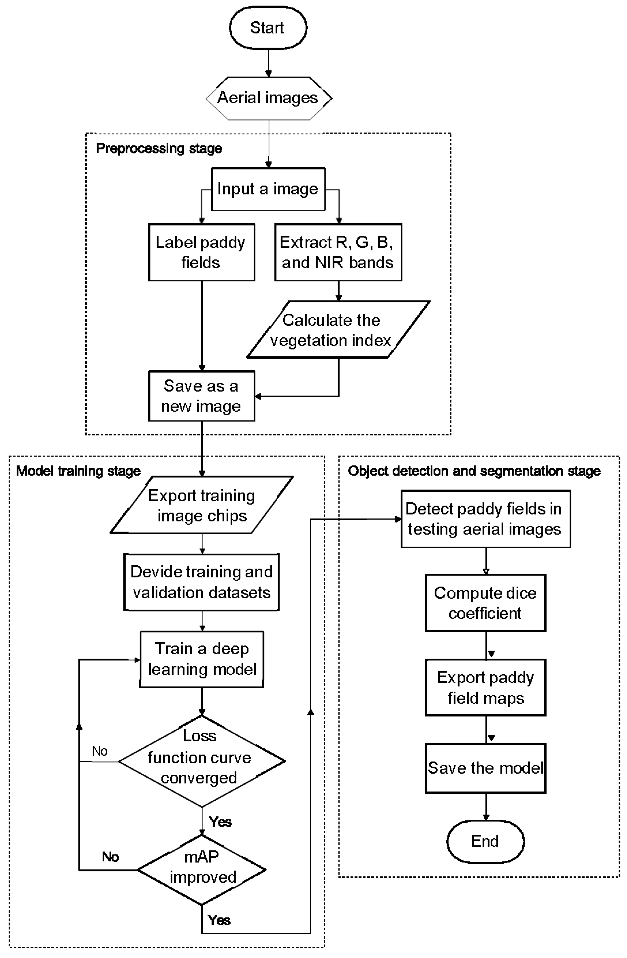
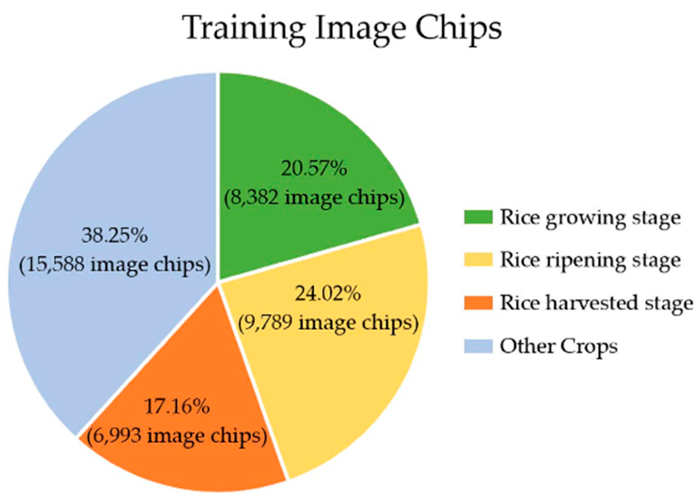
To avoid overburdening computing resources, aerial images with a broad frame and many pixels must be cropped into smaller pieces before conducting a deep learning model training process. Therefore, we obtained orthorectified aerial images with the size of 11,460 × 12,260 pixels, finished image preprocessing, and edited corresponding paddy field label files before cropping them into image chips. These image chips were cropped from each original aerial image from left to right and top to bottom with a fixed size of 550 × 550 pixels. If an image cannot be cropped on its own, the remaining area will be filled with black pixels with a value of zero. To further enhance the training dataset, we implemented a data augmentation technique. This involved rotating the image chips by 120 degrees and 240 degrees, effectively tripling the total number of image chips. Consequently, more than 18,000 training image chips were generated, utilizing 14 out of the 17 available aerial images. These cropped training image chips did not overlap and were assembled into a training dataset. We generated seven datasets from aerial images with different band combinations, including RGB, RGB + NIR, RGB + NDVI, RGB + CMFI, RGB + DVI, RGB + RVI, and RGB + GRVI, which were subsequently used for paddy field detection and segmentation model training. The research pipeline of this study is depicted in Figure 2, featuring three primary stages: preprocessing, model training, and object detection and segmentation. During the preprocessing stage, we computed vegetation indices and adjusted the band combination of the aerial images. In the subsequent model training stage, we utilized ArcGIS Pro to train Mask RCNN instance segmentation models. Finally, we applied the trained models to detect paddy fields in the aerial images during the object detection and segmentation stage. The number of image chips in different categories is shown in Figure 3.

2.4. Labeled Categories

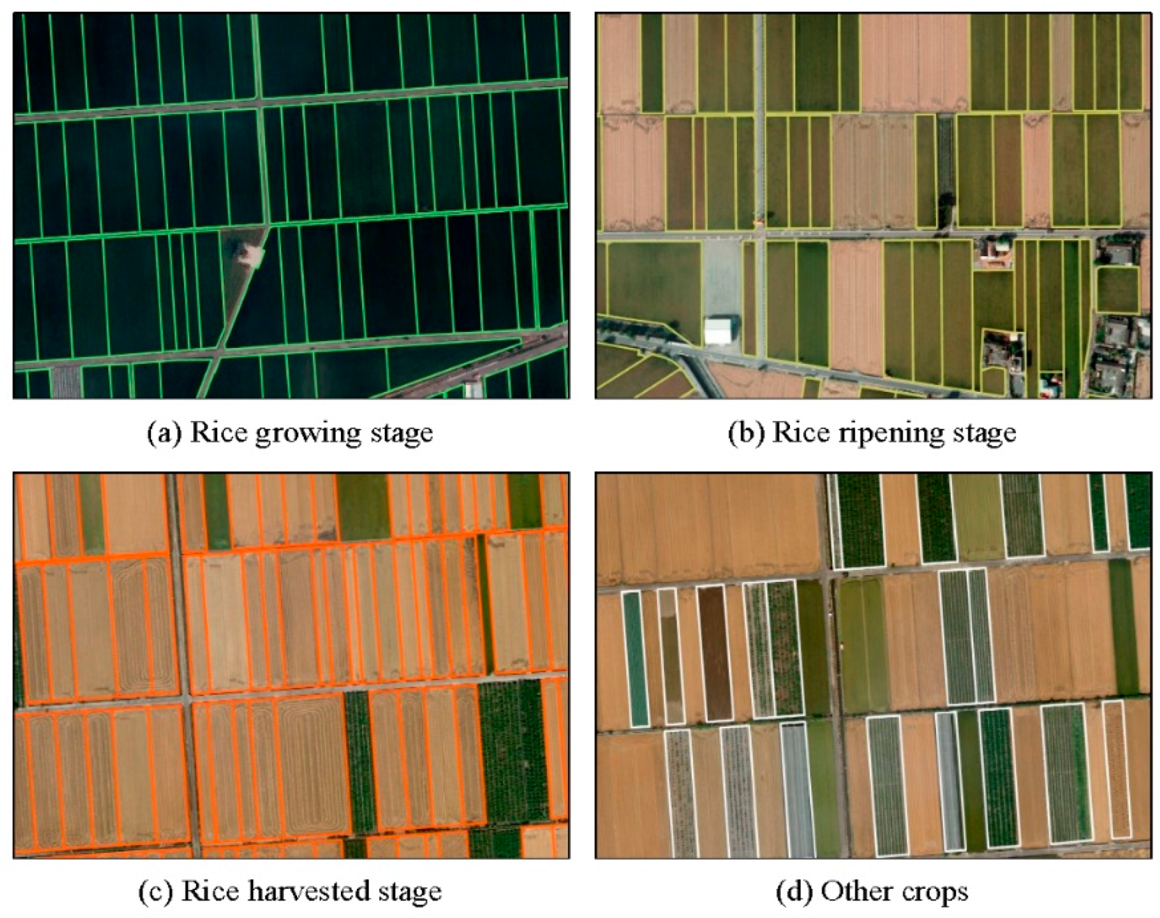
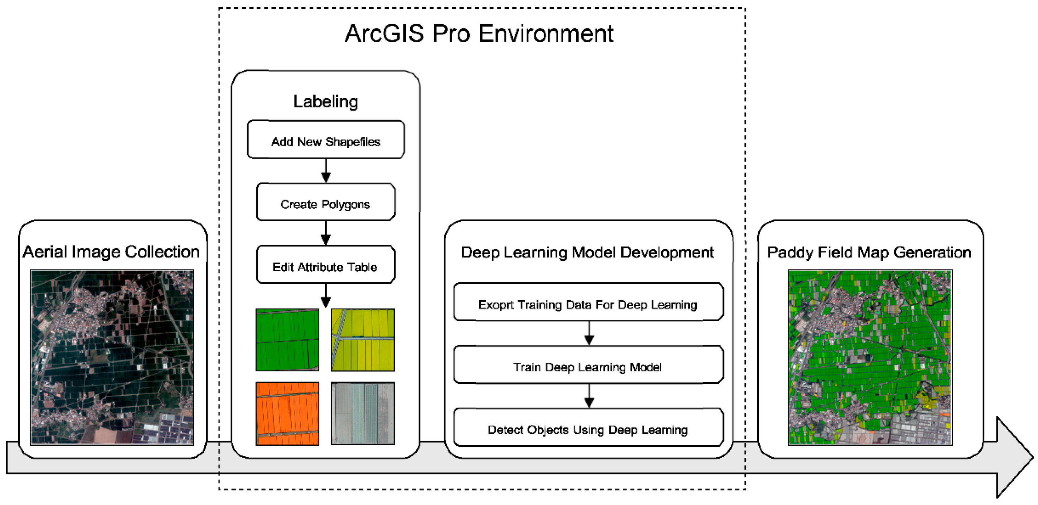
Experts from TARI have rich practical experience in paddy field identification and rice phenological stage classification. According to the suggestions provided by the experts from TARI, and different characteristics such as colors of paddy fields in aerial images, we defined four label categories listed in Table 5, including three rice phenological stage classes and one other crops class. Figure 4a–c shows examples of the three labeled categories that correspond to various stages of rice cultivation: growing, ripening, and harvested stages. Figure 4d gives an example of other crops. In addition, the paddy fields were labeled in polygons and classified by editing the attribute table in the ArcGIS Pro software. We also described the different categories in more detail as follows:

2.4.1. Rice Growing Stage

To simplify categorization, we merged the vegetative and reproductive stages into a single growing stage. In aerial images, paddy fields in this stage typically exhibit a dark green hue, sometimes appearing almost black. An example of what growing stage paddy fields look like is shown in Figure 4a, marked with green boundaries.

2.4.2. Rice Ripening Stage

In aerial images, paddy fields in the ripening stage typically display a yellow or yellow−green color. However, distinguishing them from fields in the growing stage can be visually challenging. To address this, we incorporated vegetation indices to bolster the model’s capacity for differentiation. Figure 4b depicts paddy fields in the ripening stage, marked with yellow boundaries.

2.4.3. Rice Harvested Stage

While not directly related to the phenological stages of rice, this category can still provide insights into the harvesting status of paddy fields. Aerial images reveal that, after the rice harvest, the soil in paddy fields takes on an earthy-yellow hue. Additionally, scorch marks may be visible due to farmers’ burning of rice straws. An example of this harvested stage is depicted in Figure 4c, marked with orange boundaries.

2.4.4. Other Crops

The rationale behind this category is that the traits of farmlands adjacent to paddy fields, which may be sowed with other crops, could resemble those of paddy fields. Inaccurate labeling files could compromise the deep learning model’s detection precision. As a solution, we labeled the farmlands next to paddy fields to enhance the model’s ability to differentiate between rice and other crops. For instance, the farmlands marked with white boundaries in Figure 4d do not qualify as paddy fields and are therefore classified under the other crops category.

2.5. Mask RCNN

In this study, we opted for the Mask RCNN instance segmentation model over object detection or semantic segmentation models for two primary reasons. Firstly, traditional object detection models utilize bounding boxes to present detection results. However, as paddy fields in aerial images are generally closely adjacent, capturing each paddy field area entirely in the cropped training sample images is impossible, resulting in many broken blocks. Additionally, the models were trained using cropped image chips and subsequently tested on large-scale, uncropped raw images. Notably, the size of the training sample images is significantly smaller than that of the aerial images used for testing. The current computing resources used in this study cannot support image detection areas that are too large. Hence, the sliding window method, which uses a fixed-size moving unit to scan the entire aerial image from left to right and from top to bottom, was employed to detect each scanned area. As a result, the output bounding boxes often identify an entire paddy field as multiple broken parts, making the overall detection results messy and challenging to interpret. Secondly, semantic segmentation models only provide classification information between pixels, making subsequent editing and integration operations of the paddy field map challenging. In contrast, instance segmentation models can distinguish individual regions of the same category, enabling different paddy field regions to be entirely cut out and treated as independent parts. Considering the above reasons, we employed the Mask RCNN model, which is the only instance segmentation model available in the ArcGIS Pro environment. We aimed to address the challenges associated with object detection and semantic segmentation in paddy fields. Our objective was to achieve accurate identification and segmentation of paddy field regions. To achieve this, we utilized the Mask RCNN model and trained it using the parameters outlined in Table 6. To ensure the robustness and accuracy of our model, we implemented a thorough evaluation process. Initially, during the model training phase, we partitioned the images into training and validation image chips at a ratio of 4:1. This division allowed us to train the model on a substantial dataset while reserving a portion for validation purposes. The validation dataset consists of 20% of the total image chips for each labeled category. To prevent overfitting, the early stopping mechanism evaluates the validation loss in every epoch. If the validation loss fails to decrease for five consecutive epochs, the model training process is halted. Upon completing the model training, we proceeded with the testing phase. For this stage, we employed three additional aerial images, each possessing dimensions of 11,460 by 12,260. These images were carefully selected to provide diverse and representative data for evaluating the performance of our model. By conducting testing on these independent images, we aimed to assess the generalization and effectiveness of our proposed approach in real-world scenarios.
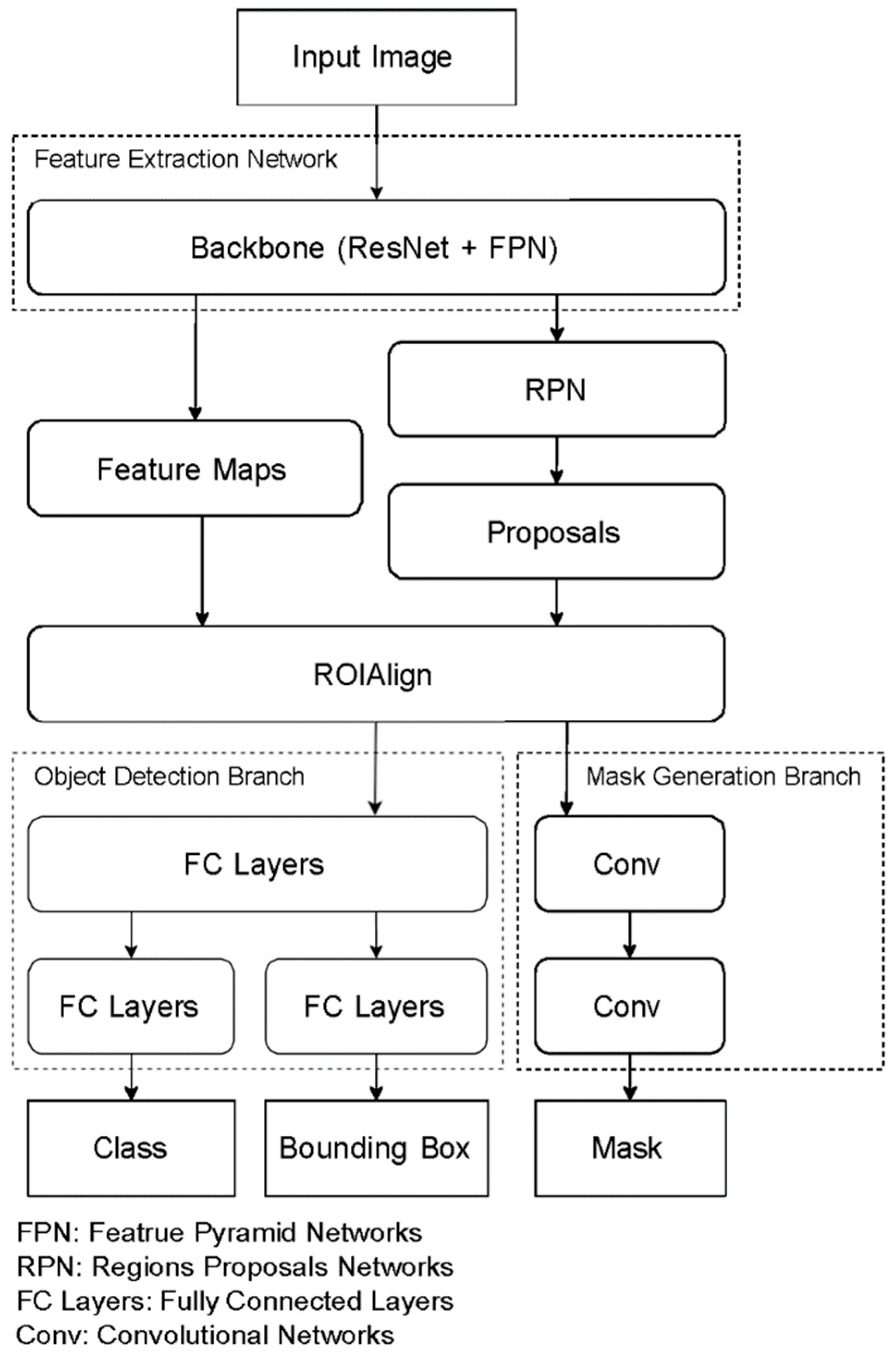
The Mask RCNN model [19] is the instance segmentation model built based on the Faster RCNN model [39] with minor modifications for object segmentation. The first modification is to replace the original ROIPooling method with ROIAlign to align the original image and feature maps better, resulting in more accurate bounding box positioning and target object detection. Secondly, a new branch consisting of two fully convolutional networks (FCN) is added to the original Faster RCNN model for generating masks. This branch utilizes a convolution and deconvolution layer architecture to perform semantic segmentation on each detected object. The Mask RCNN model architecture, as shown in Figure 5, includes a CNN-based feature extraction backbone consisting of a feature pyramid network (FPN) and ResNet. FPN enables multi-scale feature extraction for robust object detection and segmentation, while ResNet is a deep neural network with residual connections that facilitates the training of deep networks. This backbone generates feature maps by extracting local features from the input image. The subsequent regional proposal network (RPN) predicts potential target object regions using anchor boxes of various sizes and calculates the IOU loss between these predicted regions and the ground truth labels to evaluate their performance. The model then selects the most accurately predicted regions based on sorted IOU loss values for subsequent category classification, bounding box prediction, and mask generation tasks. Therefore, as a two-stage object detection and segmentation model, Mask RCNN can accurately identify and segment target objects in images.
The Mask RCNN model utilizes three different loss functions for its components. The classification loss is calculated using cross-entropy, the bounding box loss employs Smooth L1 loss, and the mask loss relies on average binary cross-entropy. The loss function of Mask RCNN can be written as
L = Lcls + Lbox + Lmask,
where Lcls, Lbox, and Lmask denote the classification, bounding box, and mask losses, respectively.

2.6. Equipment

In this study, we used ArcGIS Pro software to train deep learning models. ArcGIS Pro is a widely used GIS software developed by Environmental Systems Research Institute (Esri) Inc., Redlands, CA, USA, for map drawing and spatial information analysis. The built-in Python environment of ArcGIS Pro can install commonly used deep learning libraries, such as PyTorch, TensorFlow, and Scikit-learn, which support us in deep learning model training and development. Moreover, by using the geoprocessing and visualization tools in the software, our deep learning models could be applied to a wide range of remote sensing images for the paddy field detection and segmentation task. Figure 6 illustrates the workflow on ArcGIS Pro. After importing the aerial images, we employed editing tools to label the paddy field area. Then, we utilized the deep learning toolboxes available in the software to develop the instance segmentation models. Finally, we evaluated the model training results by using test images. We utilized the toolboxes in ArcGIS Pro to develop deep learning models in this study. To prepare the images for model training, we employed the “Export Training Data for Deep Learning” toolbox to crop them appropriately. Next, we utilized the “Train Deep Learning Model” toolbox for training our instance segmentation model. Finally, we used the “Detect Objects Using Deep Learning” toolbox to identify and locate the target area in the image. As an example, we used this approach to identify and locate paddy fields in aerial images. By leveraging this toolbox, we were able to accurately detect and segment the paddy fields, which can have important implications for agricultural planning and resource management. Furthermore, Table 7 provides information on the versions of the deep learning libraries, ArcGIS Pro, and Python used. It also includes details about the computer specifications and computing resources utilized in this study.

2.7. Evaluation Metrics

In this study, we employed average precision (AP) and mean average precision (mAP) as the evaluation metrics for assessing the performance of the deep learning model in classifying rice phenological stages. In addition, the Dice coefficient was utilized to evaluate the model’s segmentation performance in dividing paddy field regions. We used P for precision and r for recall. The AP is defined as the area under the precision-recall curve. The AP is formulated as follows:
AP = 0 1 P ( r ) d r .
Moreover, considering the presence of multiple categories within the training data, it is common to calculate the arithmetic mean of AP values for each category. This mAP metric serves as an evaluation measure for the model’s overall classification performance across all categories.
On the other hand, precision and recall are calculated in the case of image segmentation true positive (TP) denotes the area correctly segmented by the model, true negative (TN) shows the area that the model chooses not to identify, false negative (FN) represents the area that the model does not successfully detect, and false positive (FP) indicates the area that the model segment incorrectly. Based on those above mentioned, the precision and recall are formulated as follows:
Precision = TP TP + FP
and
Recall = TP TP + FN
The Dice coefficient is utilized in this study to evaluate the model’s segmentation performance. It measures the overlap between the original label area and the area segmented by the model. Let A represent the ground truth label area, and B denote the model segmentation area. The Dice coefficient can be calculated as:
Dice   Coefficient = 2 TP 2 TP + FP + FN = 2 | A B | | A | + | B |

3. Results

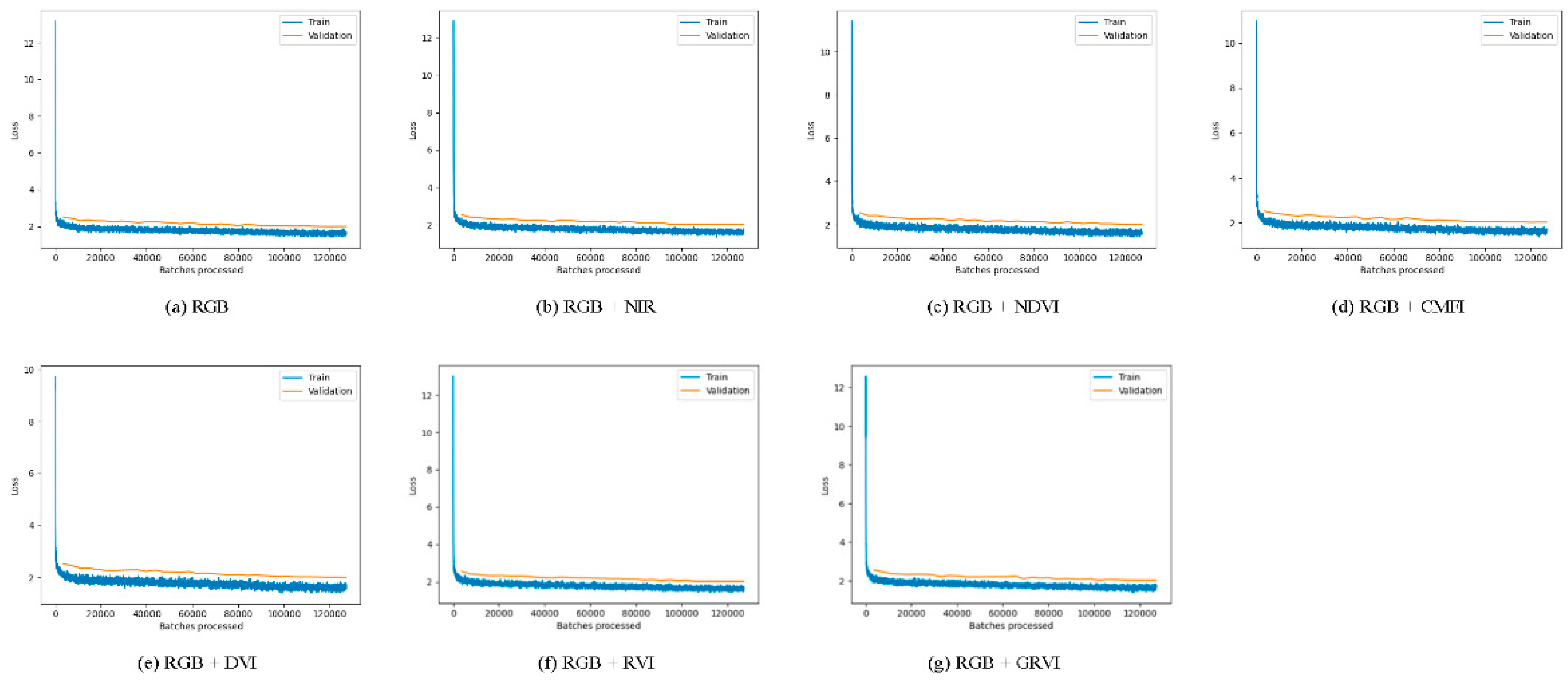
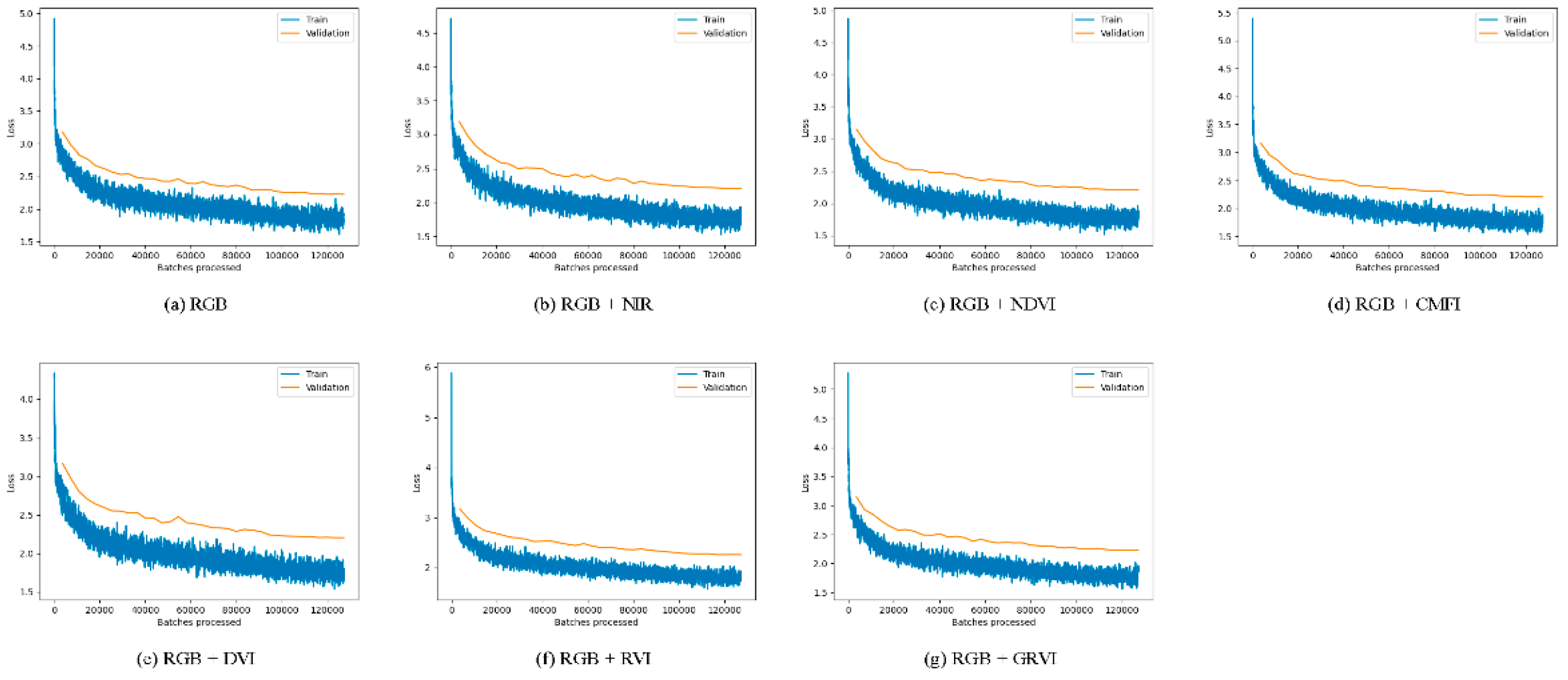
For evaluating the training performance of the deep learning model, we used AP for a single category and mAP for the overall model performance across all categories. For the presented results, the IOU value was set at 0.5. The results of various Mask RCNN models, trained with ResNet-50 and ResNet-101 backbones on images with different vegetation indices, are presented in Table 8. The table reveals that the model trained on the RGB + DVI image dataset exhibited the highest mAP of 74.01%, followed by RGB + NIR with an mAP of 73.81%, and in third place is RGB + GRVI, with an mAP of 73.72%. Furthermore, the models trained with ResNet-50 backbone performed better than those trained with ResNet-101, with an average mAP of approximately 2.5% higher. Hence, the models trained with the ResNet-50 backbone outperformed those trained with ResNet-101, with RGB + DVI, RGB + NIR, and RGB + GRVI being the best performers in the paddy field image dataset. Figure 7 and Figure 8 depict the gradual convergence of the loss curve during the training of the Mask RCNN model using two different backbones, ResNet50 and ResNet101, along with different band combinations. The graphics are generated automatically by ArcGIS Pro once the model training is finished. The X-axis of the graphs represents the number of batches processed, and Y-axis represents the loss value.
To evaluate the segmentation performance of the models, we tested them on three aerial images that were not part of the training and validation datasets. The images had a size of 11,460 × 12,260 and were sourced from different locations: Zhutang Township in Changhua County, Xingang Township in Chiayi County, and Houbi District in Tainan City. We employed the Dice coefficient to assess the models’ performance in segmenting paddy fields.

3.1. Rice Growing Stage

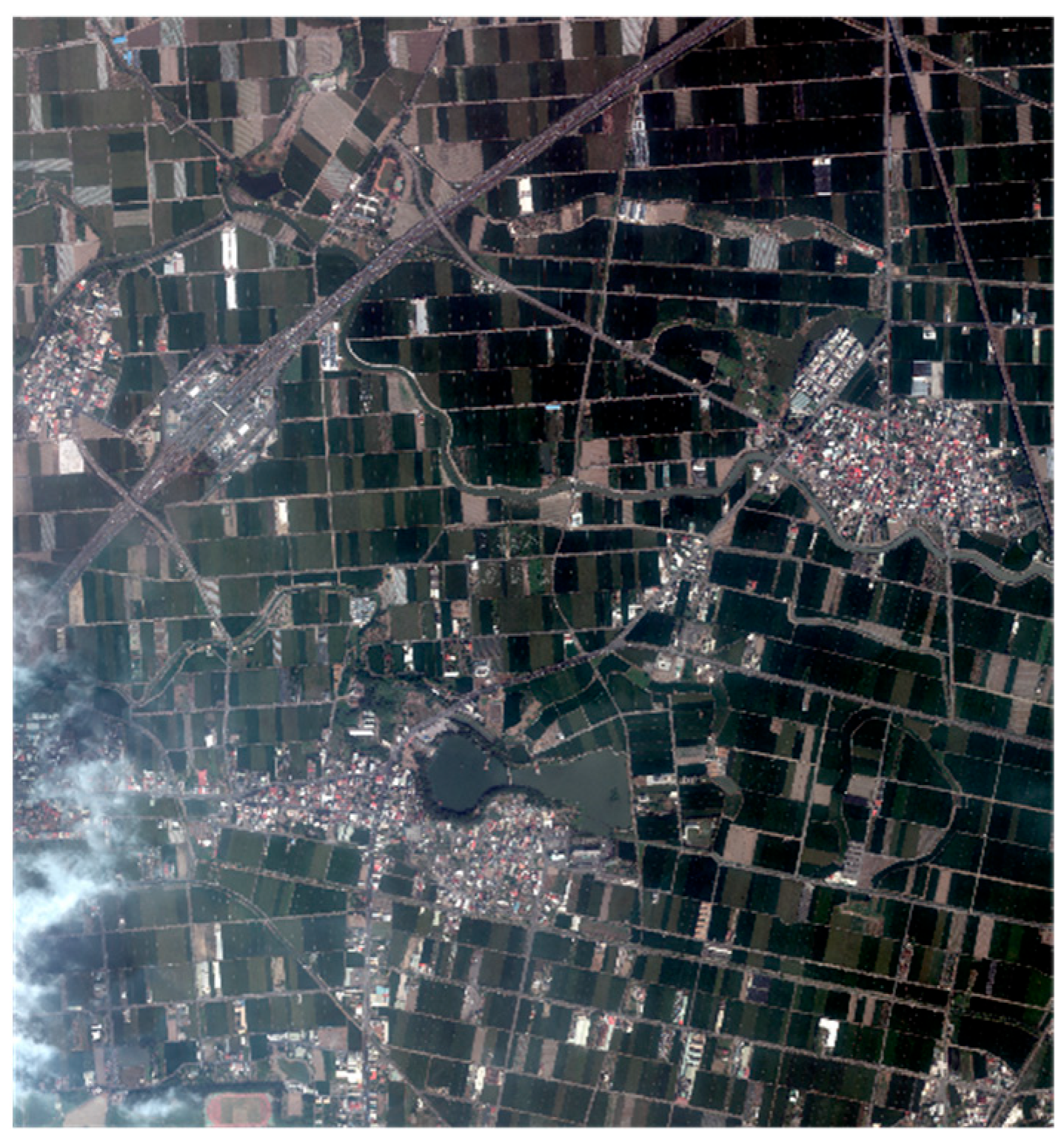
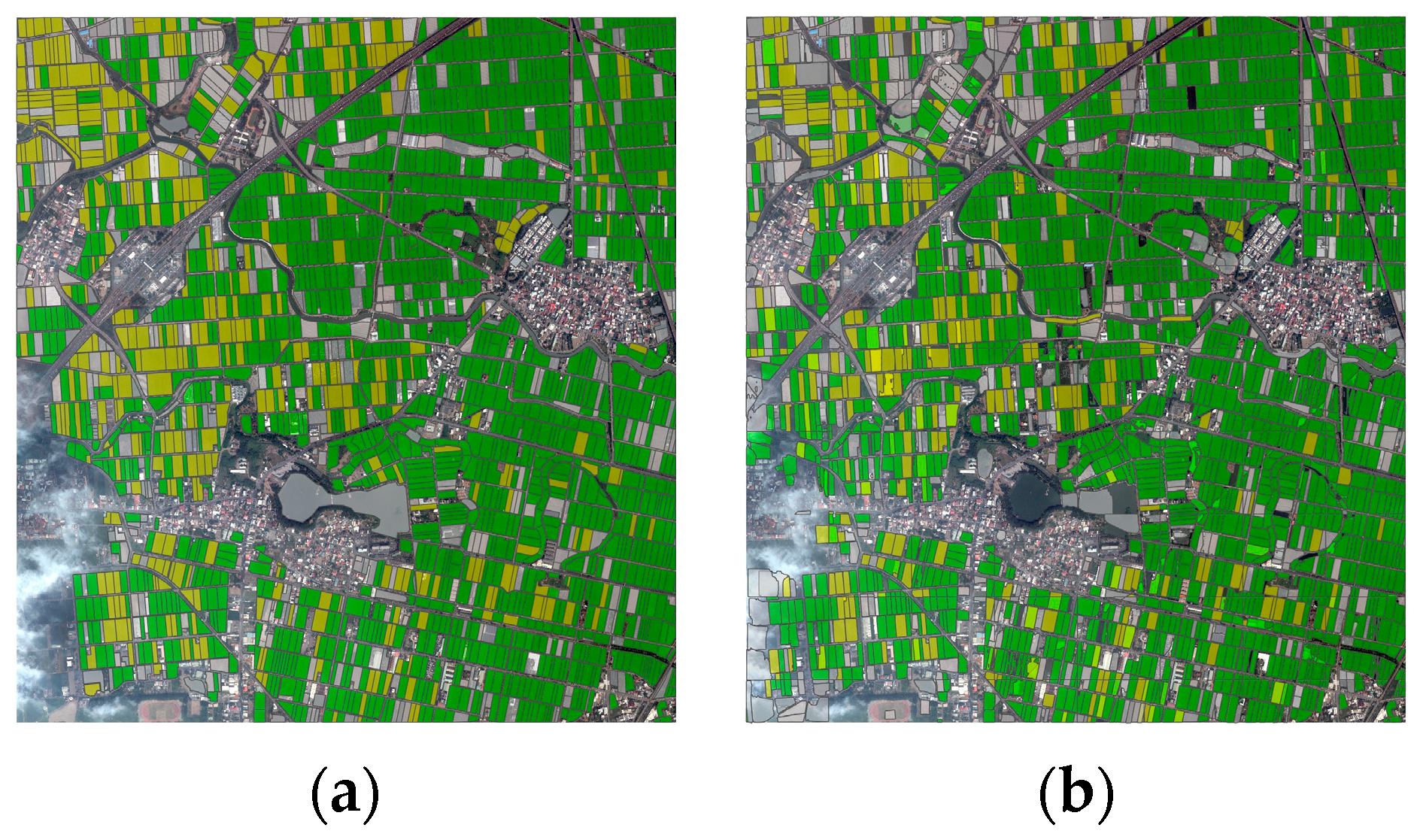
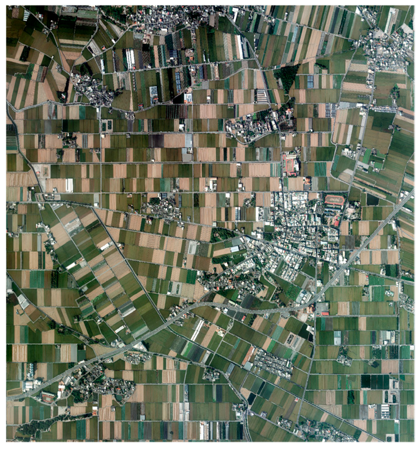
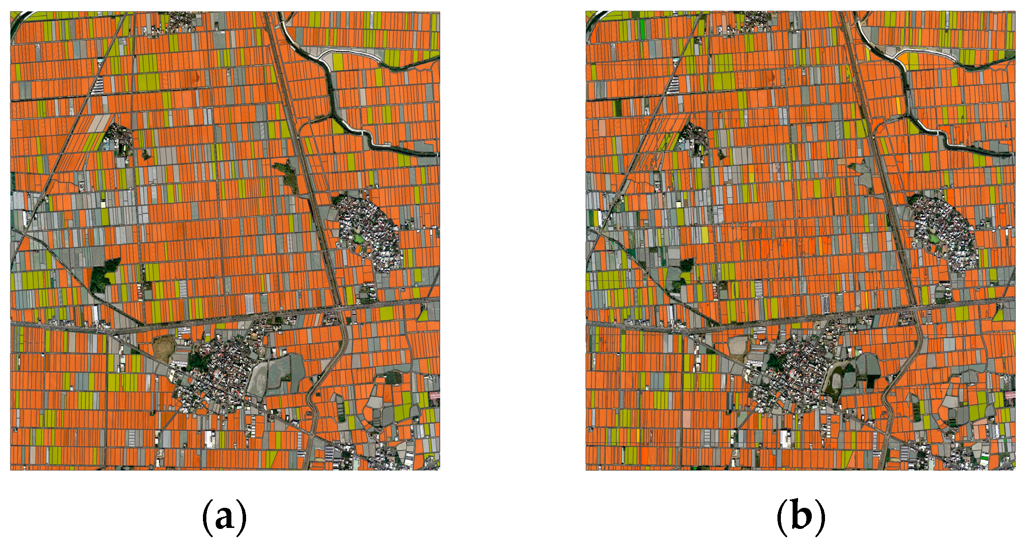
Figure 9 is the aerial image of Houbi District in Tainan City, featuring three label categories: paddy fields in rice growing and ripening stages, and other crops. The paddy fields in the rice growing stage comprise the largest number of labels and occupy the largest area, making them the primary category in this image. The Mask RCNN models trained with ResNet-50 and ResNet-101 backbones were evaluated using the average Dice coefficient of the three categories, as shown in Table 9. Results indicate that the model trained on the RGB + CMFI image dataset using the ResNet-50 backbone achieved the best average Dice coefficient of 79.59%. Furthermore, RGB + CMFI performed within the top three Dice coefficients for each category, surpassing other models. The superior performance of RGB + CMFI may be attributed to the CMFI vegetation index, which standardizes the NDVI value between 0 and 1, resulting in better model learning outcomes. This makes it a reliable indicator for assessing rice growth in the growing stage. Figure 10 shows the ground truth label and the detection result using the model trained with RGB + CMFI dataset.

3.2. Rice Ripening Stage

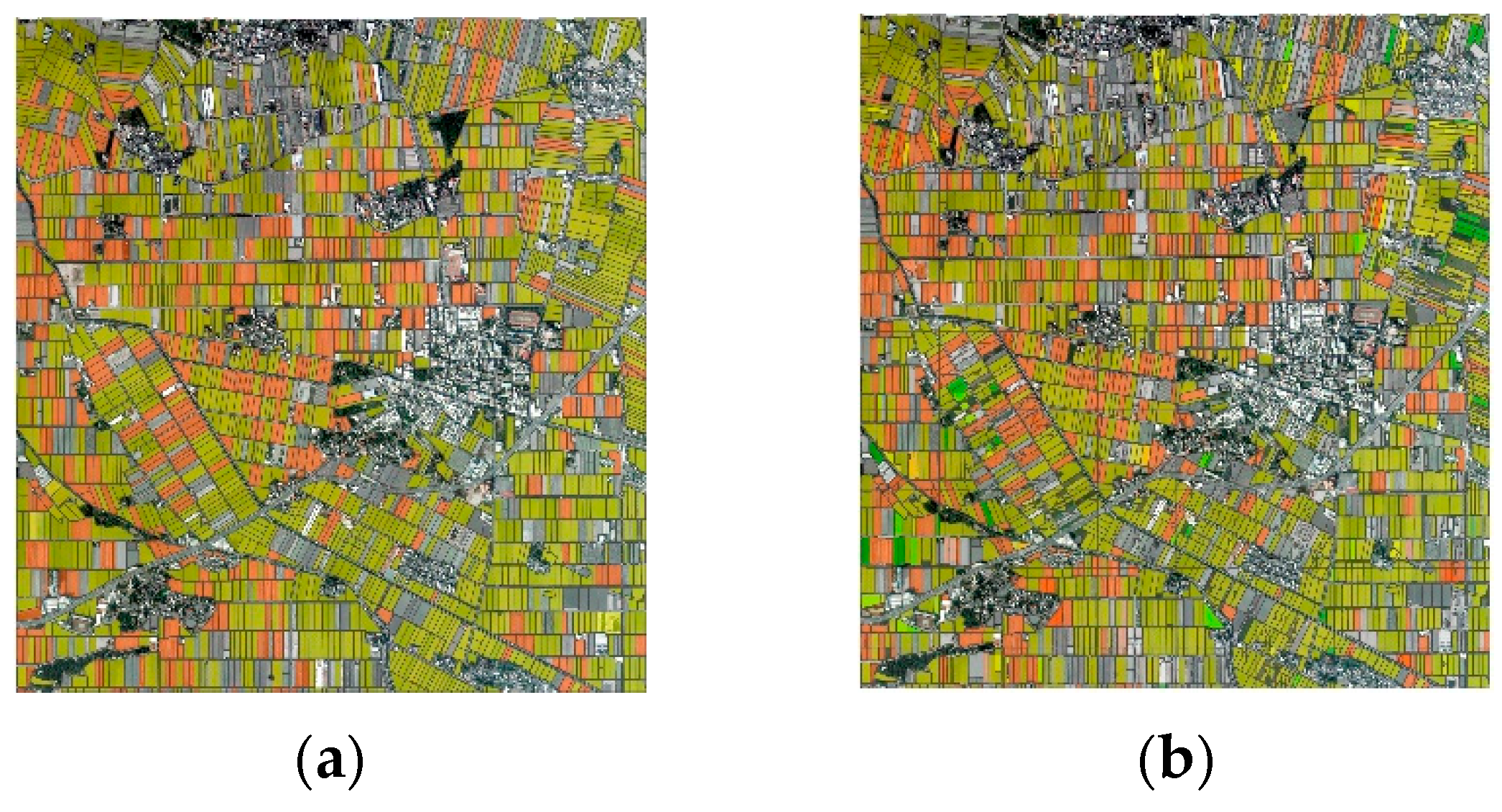
Figure 11 is the image that depicts three distinct label categories: paddy fields during the rice ripening, harvested stages, and other crops. Among these categories, the paddy fields in the ripening stage occupy the most significant area, thus being considered the most prominent feature in this image. The image was employed to evaluate various models’ detection and segmentation capabilities for identifying paddy fields in the ripening stage. The performance of the Mask RCNN models, trained with the ResNet-50 and ResNet-101 backbones, is presented in Table 10. The results demonstrate that the model trained on the RGB + NIR image dataset achieved the highest average Dice coefficient of 89.71%, indicating that the inclusion of NIR information aids in detecting and segmenting the paddy fields in this aerial image. In contrast, the comparison between NIR and various vegetation indices reveals an improvement in the Dice coefficient by approximately 1%. This could be attributed to the selected vegetation indices emphasizing green vegetation, which may not be relevant for most paddy fields during the rice ripening stage. Instead, using the NIR band directly may better reflect the transition of the rice growth status during the rice ripening stage. Figure 12 shows the ground truth label and the detection result using the model trained with the RGB + NIR dataset.

3.3. Rice Harvested Stage

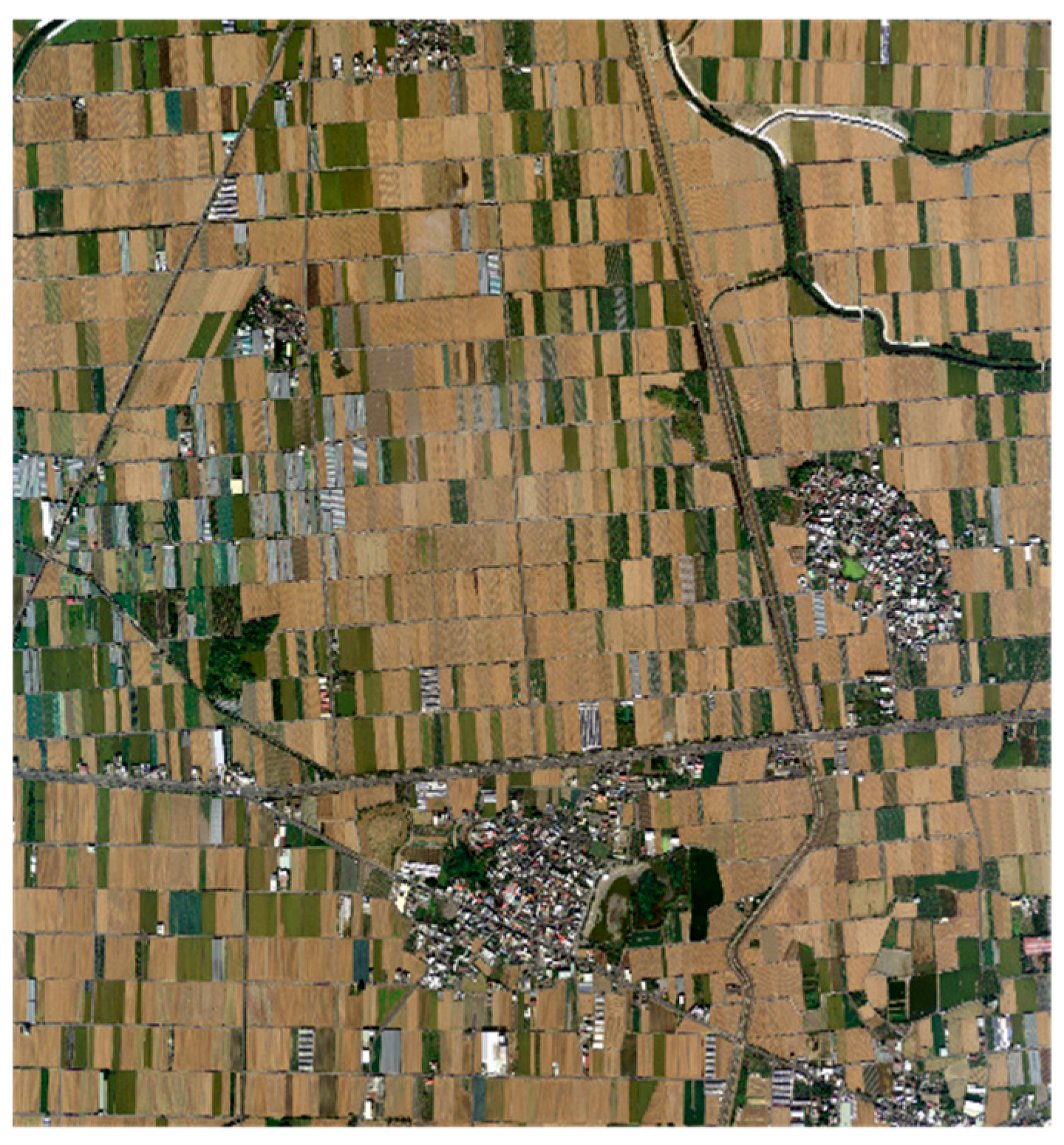
Figure 13 is the image that consists of three label categories: paddy fields in the rice ripening and harvested stages, and other crops. Of these categories, the paddy fields in the harvested stage are the most numerous and occupy the largest area, thereby being the most prominent in this image. This image was utilized to evaluate the detection and segmentation performance of various models for identifying paddy fields in the harvested stage. Table 11 presents the Dice coefficient for each category, computed using the Mask RCNN models trained with ResNet-50 and ResNet-101 backbones. Among the models, the one trained on the RGB + GRVI image dataset with the ResNet-50 backbone displayed the best average Dice coefficient of 87.94%, surpassing all other categories. This suggests that the GRVI, a vegetation index obtained by combining the G and R bands, may better distinguish paddy fields with vegetation cover from bare soil. Incorporating GRVI in the deep learning models enhances their ability to detect and segment paddy fields more efficiently in the harvested stage. Figure 14 shows the ground truth label and the detection result using the model trained with the RGB + GRVI dataset.

4. Discussion

This study created detailed paddy field image datasets labeled by different rice phenological stages and used various vegetation indices to enhance the models’ paddy field detection and segmentation performance.
DVI measures the difference between the reflectance of NIR and green light. Unlike NDVI, DVI values are not normalized and can range from negative to positive, with positive values indicating denser vegetation cover. DVI can be useful in identifying vegetation cover in the later growth stages when vegetation cover may not be entirely green. However, DVI may not capture the nuances of vegetation cover in different phenological stages as effectively as other indices.
Table 12 shows that the Mask RCNN model with the ResNet-50 backbone trained on the RGB + CMFI image dataset performed well in assessing the rice growing stage. ResNet-50 and ResNet-101 are two popular CNN architectures commonly used in computer vision tasks. ResNet-101 is a deeper and more complex version of ResNet-50, with 101 layers compared to 50 layers in ResNet-50. However, deeper neural networks are not always better for every task. The performance of a neural network depends on the complexity of the task and the characteristics of the dataset. In the case of paddy field images used for assessing rice growing stage, the characteristics of the images are not too complex, which means that a deeper network like ResNet-101 may not provide improved performance over ResNet-50. In fact, using a deeper network with more parameters can sometimes lead to overfitting, where the model becomes too complex and starts to memorize the training data instead of learning general features. This can result in poor performance on new, unseen data. The results suggest that the Mask RCNN model with ResNet-50 backbone trained on RGB + CMFI image dataset performed well in assessing the rice growing stage. This means that ResNet-50 was able to capture the relevant features of the paddy field images and provide accurate predictions. Therefore, ResNet-50 is considered better than ResNet-101 for this specific task.
The CMFI vegetation index standardizes the NDVI value between 0 and 1, resulting in better model learning outcomes. Vegetation indices like NDVI are commonly used in remote sensing and computer vision applications to identify vegetation cover and monitor crop health. However, NDVI values can vary significantly depending on the type of vegetation, soil moisture, and other environmental factors. This variability can make it challenging for deep learning models to learn generalizable features that can accurately distinguish between different crops. The CMFI vegetation index is a modified version of the NDVI that addresses this variability by standardizing the NDVI values between 0 and 1. This normalization makes the CMFI index less sensitive to the variability in NDVI values and provides a more consistent representation of vegetation cover. By using RGB+CMFI dataset, the deep learning model is able to leverage the complementary information from both RGB and CMFI channels, which can improve the accuracy of the model in identifying rice at the growing stage. The standardized CMFI index provides a more consistent and reliable representation of the vegetation cover, which can help the model learn more robust and generalizable features.
As for the rice ripening stage, the model with RGB + NIR bands worked better than other models. The NIR band can penetrate deeper into the canopy, providing information on the internal structure of the plants and their health status. The RGB channels, on the other hand, capture information on the color and texture of the rice fields. Therefore, combining both RGB and NIR channels can help the model identify and segment the rice fields accurately in this stage. Based on the performance comparison, it appears that utilizing NIR information directly is more effective for most paddy fields in the rice ripening stage, while other vegetation indices tend to place more emphasis on green vegetation cover. Therefore, utilizing NIR information directly may be the preferable approach for detecting paddy fields at the ripening stage.
GRVI measures the ratio of the difference between the reflectance of green and red light to the sum of the reflectance of green and red light. GRVI can highlight the seasonal changes in surface soil and vegetation by combining red and green light. GRVI can be useful in distinguishing harvested areas in the later growth stages of rice fields. As a result, it performs well in distinguishing harvested areas. We observed that the model, trained on images combining RGB and GRVI, exhibited outstanding detection and segmentation abilities in the rice harvested stage. Its performance surpassed the model trained solely on RGB images. This finding is insightful and suggests that, in scenarios when the NIR band is not acquired, we can leverage the available RGB bands to compute GRVI vegetation indices and enhance the precision of identifying surface vegetation growth changes. As a result, different deep learning models trained on images with various band combinations can be utilized for detecting and segmenting paddy fields according to different rice phenological stages. The detection and segmentation results provide insight into the rice growth status in different phenological stages and can help generate rice maps and estimate yield and harvested area.

5. Conclusions

This study explored the effectiveness of different image datasets and improved deep learning models’ detection and segmentation performance by using different vegetation indices for different rice phenological stages. The results showed that different models trained on images with different band combinations could detect and segment paddy fields for different stages, providing a reliable basis for estimating rice yield and harvested area. It can be concluded that RGB + CMFI is more effective during the growing stage, while RGB + NIR may be more useful during the ripening stage. Incorporating the RGB + GRVI vegetation index improves the efficiency of detection and segmentation during the harvested stage. Additionally, the study proposed a method to develop detection tools for specific crop farmlands based on the existing environment of ArcGIS Pro software, which can reduce the workload of researchers and improve the efficiency of land use surveys.

Author Contributions

Conceptualization, Y.-S.C. and C.-Y.C.; methodology, Y.-S.C.; software, Y.-S.C.; validation, Y.-S.C.; formal analysis, Y.-S.C. and C.-Y.C.; investigation, Y.-S.C.; writing—original draft preparation, Y.-S.C.; writing—review and editing, C.-Y.C.; visualization, Y.-S.C.; supervision, C.-Y.C.; project administration, C.-Y.C.; funding acquisition, C.-Y.C. All authors have read and agreed to the published version of the manuscript.

Funding

This study received external support from the Information Management Center of the Council of Agriculture, Executive Yuan, R.O.C. under Grant No. 110AS-9.1.1-I-i2.

Data Availability Statement

The authors have no rights to share the data.

Acknowledgments

The authors thank the staff of the Taiwan Agricultural Research Institute, Council of Agriculture, Executive Yuan, R.O.C., for their support of aerial imagery.

Conflicts of Interest

The authors declare no conflict of interest. The funders had no role in the design of the study; in the collection, analyses, or interpretation of data; in the writing of the manuscript; or in the decision to publish the results.

Abbreviations

The following abbreviations are used in this manuscript:
APAverage precision
BBlue
COACouncil of Agriculture
CMFICropping management factor index
CNNConvolutional neural network
DCNNDeep convolutional neural network
DOTADataset for object detection in aerial images
DVIDifference vegetation index
EsriEnvironmental Systems Research Institute, Inc.
FNFalse negative
FCNFully convolutional networks
FPFalse positive
FPNFeature pyramid networks
GGreen
GISGeographic information system
GLCMGray-level co-occurrence matrix
GRVIGreen-red vegetation index
iSAIDInstance segmentation in aerial images dataset
LULCLand use and land cover
mAPMean average precision
NDVINormalized difference vegetation index
NIRNear-infrared
RRed
RCNNRegion-based convolutional network
RPNRegional proposal network
ROIRegion of interest
RVIRatio vegetation index
RFRandom forest
SVMSupport vector machine
TARITaiwan Agricultural Research Institute
TNTrue negative
TPTrue positive

References

  1. Council of Agriculture, Executive Yuan, T. Agricultural Statistics. 2022. Available online: https://agrstat.coa.gov.tw/sdweb/public/indicator/Indicator.aspx (accessed on 5 November 2022).
  2. Moldenhauer, K.; Slaton, N. Rice growth and development. Rice Prod. Handb. 2001, 192, 7–14. [Google Scholar]
  3. Jo, H.W.; Lee, S.; Park, E.; Lim, C.H.; Song, C.; Lee, H.; Ko, Y.; Cha, S.; Yoon, H.; Lee, W.K. Deep learning applications on multitemporal SAR (Sentinel-1) image classification using confined labeled data: The case of detecting rice paddy in South Korea. IEEE Trans. Geosci. Remote Sens. 2020, 58, 7589–7601. [Google Scholar]
  4. Ma, L.; Liu, Y.; Zhang, X.; Ye, Y.; Yin, G.; Johnson, B.A. Deep learning in remote sensing applications: A meta-analysis and review. ISPRS J. Photogramm. Remote Sens. 2019, 152, 166–177. [Google Scholar]
  5. Xia, G.S.; Bai, X.; Ding, J.; Zhu, Z.; Belongie, S.; Luo, J.; Datcu, M.; Pelillo, M.; Zhang, L. DOTA: A large-scale dataset for object detection in aerial images. In Proceedings of the IEEE Conference on Computer Vision and Pattern Recognition, Salt Lake City, UT, USA, 13–23 June 2018; pp. 3974–3983. [Google Scholar]
  6. Waqas Zamir, S.; Arora, A.; Gupta, A.; Khan, S.; Sun, G.; Shahbaz Khan, F.; Zhu, F.; Shao, L.; Xia, G.S.; Bai, X. isaid: A large-scale dataset for instance segmentation in aerial images. In Proceedings of the IEEE/CVF Conference on Computer Vision and Pattern Recognition Workshops, Long Beach, CA, USA, 16–17 June 2019; pp. 28–37. [Google Scholar]
  7. Helber, P.; Bischke, B.; Dengel, A.; Borth, D. Eurosat: A novel dataset and deep learning benchmark for land use and land cover classification. IEEE J. Sel. Top. Appl. Earth Obs. Remote Sens. 2019, 12, 2217–2226. [Google Scholar]
  8. Hoeser, T.; Bachofer, F.; Kuenzer, C. Object detection and image segmentation with deep learning on Earth observation data: Areview—Part 2: Applications. Remote Sens. 2020, 12, 3053. [Google Scholar]
  9. Audebert, N.; Le Saux, B.; Lefèvre, S. Segment-before-detect: Vehicle detection and classification through semantic segmentation of aerial images. Remote Sens. 2017, 9, 368. [Google Scholar]
  10. Badrinarayanan, V.; Kendall, A.; Cipolla, R. Segnet: A deep convolutional encoder-decoder architecture for image segmentation. IEEE Trans. Pattern Anal. Mach. Intell. 2017, 39, 2481–2495. [Google Scholar] [PubMed]
  11. Krizhevsky, A.; Sutskever, I.; Hinton, G.E. Imagenet classification with deep convolutional neural networks. Commun. ACM 2017, 60, 84–90. [Google Scholar]
  12. Simonyan, K.; Zisserman, A. Very deep convolutional networks for large-scale image recognition. arXiv 2014, arXiv:1409.1556. [Google Scholar]
  13. Yin, S.; Li, H.; Teng, L. Airport detection based on improved faster RCNN in large scale remote sensing images. Sens. Imaging 2020, 21, 49. [Google Scholar]
  14. Khasawneh, N.; Fraiwan, M.; Fraiwan, L. Detection of K-complexes in EEG waveform images using faster R-CNN and deep transfer learning. BMC Med. Inform. Decis. Mak. 2022, 22, 297. [Google Scholar]
  15. Li, Y.; Xu, W.; Chen, H.; Jiang, J.; Li, X. A novel framework based on mask R-CNN and Histogram thresholding for scalable segmentation of new and old rural buildings. Remote Sens. 2021, 13, 1070. [Google Scholar]
  16. Pai, M.M.; Mehrotra, V.; Aiyar, S.; Verma, U.; Pai, R.M. Automatic segmentation of river and land in sar images: A deep learning approach. In Proceedings of the 2019 IEEE Second International Conference on Artificial Intelligence and Knowledge Engineering (AIKE), Sardinia, Italy, 3–5 June 2019; IEEE: Piscataway, NJ, USA, 2019; pp. 15–20. [Google Scholar]
  17. Ronneberger, O.; Fischer, P.; Brox, T. U-net: Convolutional networks for biomedical image segmentation. In Proceedings of the International Conference on Medical Image Computing and Computer-Assisted Intervention, Munich, Germany, 5–9 October 2015; Springer: Berlin/Heidelberg, Germany, 2015; pp. 234–241. [Google Scholar]
  18. Song, S.; Liu, J.; Liu, Y.; Feng, G.; Han, H.; Yao, Y.; Du, M. Intelligent object recognition of urban water bodies based on deep learning for multi-source and multi-temporal high spatial resolution remote sensing imagery. Sensors 2020, 20, 397. [Google Scholar]
  19. He, K.; Gkioxari, G.; Dollár, P.; Girshick, R. Mask r-cnn. In Proceedings of the IEEE International Conference on Computer Vision, Venice, Italy, 22–29 October 2017; pp. 2961–2969. [Google Scholar]
  20. Huang, L.; Wu, X.; Peng, Q.; Yu, X. Depth Semantic Segmentation of Tobacco Planting Areas from Unmanned Aerial Vehicle Remote Sensing Images in Plateau Mountains. J. Spectrosc. 2021, 2021, 6687799. [Google Scholar]
  21. Chen, L.C.; Papandreou, G.; Kokkinos, I.; Murphy, K.; Yuille, A.L. Deeplab: Semantic image segmentation with deep convolutional nets, atrous convolution, and fully connected crfs. IEEE Trans. Pattern Anal. Mach. Intell. 2017, 40, 834–848. [Google Scholar] [PubMed] [Green Version]
  22. Zhao, H.; Shi, J.; Qi, X.; Wang, X.; Jia, J. Pyramid scene parsing network. In Proceedings of the IEEE Conference on Computer Vision and Pattern Recognition, Honolulu, HI, USA, 21–26 July 2017; pp. 2881–2890. [Google Scholar]
  23. Zhu, X.; Liang, J.; Hauptmann, A. Msnet: A multilevel instance segmentation network for natural disaster damage assessment in aerial videos. In Proceedings of the IEEE/CVF Winter Conference on Applications of Computer Vision, Virtual, 5–9 January 2021; pp. 2023–2032. [Google Scholar]
  24. Kontgis, C.; Schneider, A.; Ozdogan, M. Mapping rice paddy extent and intensification in the Vietnamese Mekong River Delta with dense time stacks of Landsat data. Remote Sens. Environ. 2015, 169, 255–269. [Google Scholar]
  25. Onojeghuo, A.O.; Blackburn, G.A.; Wang, Q.; Atkinson, P.M.; Kindred, D.; Miao, Y. Mapping paddy rice fields by applying machine learning algorithms to multi-temporal Sentinel-1A and Landsat data. Int. J. Remote Sens. 2018, 39, 1042–1067. [Google Scholar]
  26. Hsiao, K.; Liu, C.; Hsu, W. The Evaluation of Image Classification Methods for Rice Paddy Interpretation. J. Photogramm. Remote Sens. 2004, 9, 13–26. (In Chinese) [Google Scholar]
  27. Chang, S.; Wan, H.; Chou, Y. The Eco-friendly Evaluation Model: The Paddy Rice Image Classification through SOM and Logistic Regression by Remote Sensing Data. J. Soil Water Conserv. Technol. 2012, 7, 212–220. [Google Scholar]
  28. Kim, H.O.; Yeom, J.M. Sensitivity of vegetation indices to spatial degradation of RapidEye imagery for paddy rice detection: A case study of South Korea. GIScience Remote Sens. 2015, 52, 1–17. [Google Scholar]
  29. Wan, S.; Lei, T.; Chou, T.Y. An enhanced supervised spatial decision support system of image classification: Consideration on the ancillary information of paddy rice area. Int. J. Geogr. Inf. Sci. 2010, 24, 623–642. [Google Scholar]
  30. Lei, T.C.; Huang, S.W.C.Y.; Li, J.Y. The Comparison Study of Paddy Rice Thematic Maps Based on Parameter Classifier (mlc) and Regional Object of Knowledge Classifier (RG + ROSE). Available online: https://a-a-r-s.org/proceeding/ACRS2011/Session/Paper/P_89_9-6-16.pdf (accessed on 7 April 2023).
  31. Yang, M.D.; Tseng, H.H.; Hsu, Y.C.; Tsai, H.P. Semantic segmentation using deep learning with vegetation indices for rice lodging identification in multi-date UAV visible images. Remote Sens. 2020, 12, 633. [Google Scholar]
  32. Wang, M.; Wang, J.; Cui, Y.; Liu, J.; Chen, L. Agricultural Field Boundary Delineation with Satellite Image Segmentation for High-Resolution Crop Mapping: A Case Study of Rice Paddy. Agronomy 2022, 12, 2342. [Google Scholar]
  33. Yenchia, H. Prediction of Paddy Field Area in Satellite Images Using Deep Learning Neural Networks. Master’s Thesis, Chung Yuan Christian University, Taoyuan City, Taiwan, 2019. [Google Scholar]
  34. Environmental Systems Research Institute, ArcGIS Pro Desktop: Version 3.0.2. Available online: https://www.esri.com/en-us/arcgis/products/arcgis-pro/overview (accessed on 19 June 2022).
  35. Council of Agriculture, Executive Yuan, T. Aerial Photography Information. 2022. Available online: https://www.afasi.gov.tw/aerial_search (accessed on 23 August 2022).
  36. GmbH, V.I. UltraCam-XP Technical Specifications. 2008. Available online: http://coello.ujaen.es/Asignaturas/fotodigital/descargas/UCXP-specs.pdf (accessed on 28 October 2022).
  37. Nazir, A.; Ullah, S.; Saqib, Z.A.; Abbas, A.; Ali, A.; Iqbal, M.S.; Hussain, K.; Shakir, M.; Shah, M.; Butt, M.U. Estimation and forecasting of rice yield using phenology-based algorithm and linear regression model on sentinel-2 satellite data. Agriculture 2021, 11, 1026. [Google Scholar]
  38. Lin, C.Y.; Chuang, C.W.; Lin, W.T.; Chou, W.C. Vegetation recovery and landscape change assessment at Chiufenershan landslide area caused by Chichi earthquake in central Taiwan. Nat. Hazards 2010, 53, 175–194. [Google Scholar]
  39. Ren, S.; He, K.; Girshick, R.; Sun, J. Faster R-CNN: Towards real-time object detection with region proposal networks. Adv. Neural Inf. Process. Syst. 2015, 28, 91–99. [Google Scholar]
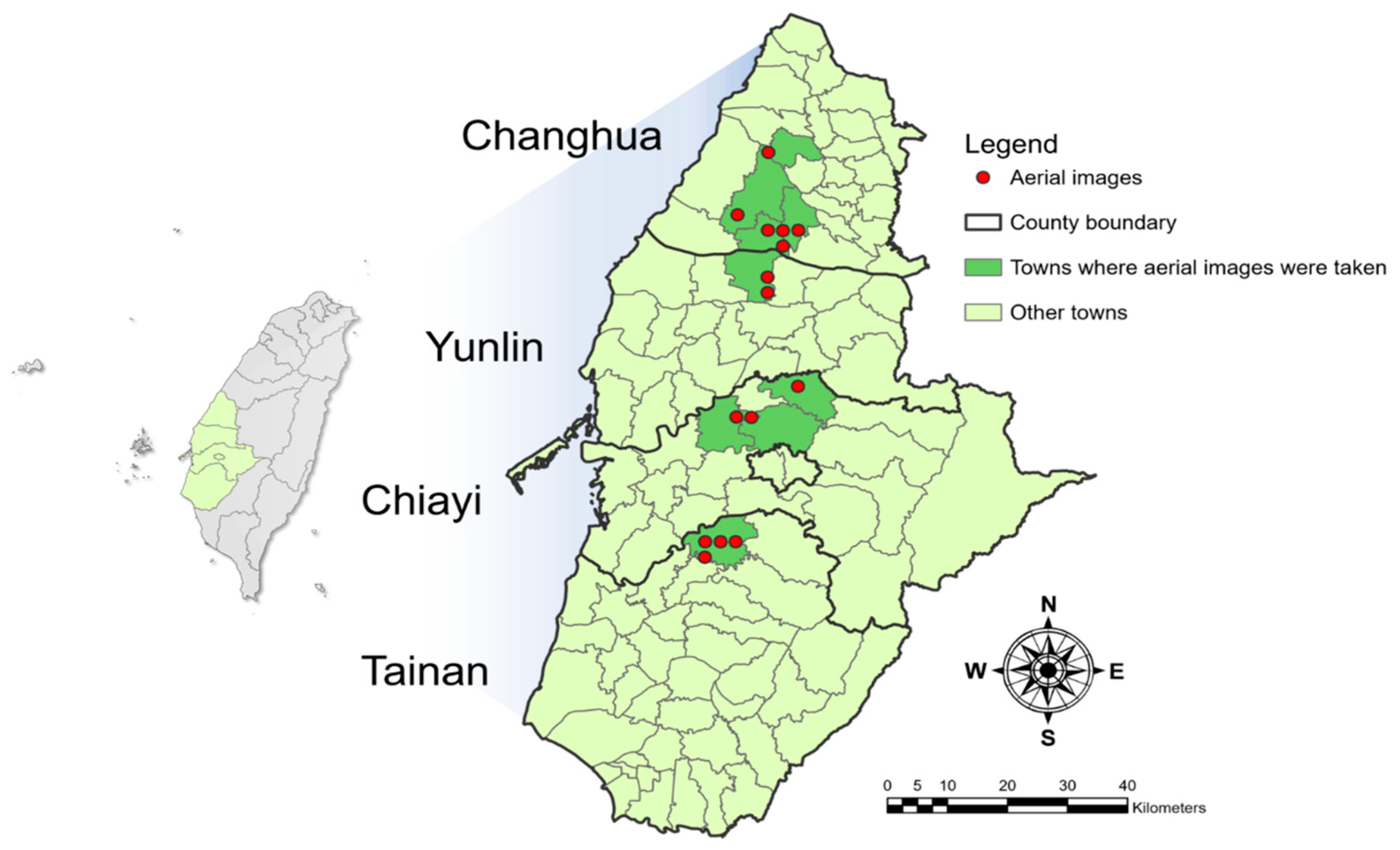
Figure 1. Regions where aerial images were taken. The red spots were the exact places where the images were taken, and the areas in dark green were townships to which the red spots belonged.
Remotesensing 15 03575 g001
Figure 2. The flow chart of this study.
Remotesensing 15 03575 g002
Figure 3. The proportions of training image chips in different categories.
Remotesensing 15 03575 g003
Figure 4. An example of labeled categories in this study.
Remotesensing 15 03575 g004
Figure 5. Mask RCNN architecture [19].
Remotesensing 15 03575 g005
Figure 6. The workflow on ArcGIS Pro in this study.
Remotesensing 15 03575 g006
Figure 7. Loss curves of Mask RCNN models with ResNet-50 trained on different image datasets.
Remotesensing 15 03575 g007
Figure 8. Loss curves of Mask RCNN models with ResNet-101 trained on different image datasets.
Remotesensing 15 03575 g008
Figure 9. The test aerial image of Houbi, Tainan (rice growing stage).
Remotesensing 15 03575 g009
Figure 10. The model which utilized the ResNet-50 backbone and was trained on the RGB + CMFI image dataset achieved the best average Dice coefficient of 79.59%. Comparison between the model’s detection and segmentation results and the ground truth. The green, yellow, and gray areas signify the paddy fields in growing, ripening, and farmlands for other crops, respectively. (a) Ground truth label. (b) Detection and segmentation result.
Remotesensing 15 03575 g010
Figure 11. The testing aerial image of Zhutang, Changhua (rice ripening stage).
Remotesensing 15 03575 g011
Figure 12. The model which utilized the ResNet-50 backbone and was trained on the RGB + NIR image dataset achieved the best average Dice coefficient of 89.71%. Comparison between the model’s detection and segmentation results and the ground truth. The yellow, orange, and gray areas signify the paddy fields in ripening, harvested, and farmlands for other crops, respectively. (a) Ground truth label. (b) Detection and segmentation result.
Remotesensing 15 03575 g012
Figure 13. The testing aerial image of Xingang, Chiayi (rice harvested stage).
Remotesensing 15 03575 g013
Figure 14. The model which utilized the ResNet-50 backbone and was trained on the RGB + GRVI image dataset achieved the best average Dice coefficient of 87.94%. Comparison between the model’s detection and segmentation results and the ground truth. The yellow, orange, and gray areas signify the paddy fields in ripening, harvested, and farmlands for other crops, respectively. (a) Ground truth label. (b) Detection and segmentation result.
Remotesensing 15 03575 g014
Table 1. Major differences between this study and existing research for paddy field detection.
Comparison ItemsExisting ResearchProposed Study
Training toolNot discussedArcGIS Pro
Band usedRGB + NDVIRGB + Optimal vegetation index
Model typeObject detectionInstance segmentation
Phenological stageNot discussedMultiple (growing, ripening, harvested)
Application environmentNot discussedArcGIS Pro
Table 2. Aerial image properties.
ItemValue
Image size11,460 × 12,260 pixels
Horizontal resolution96 dpi
Vertical resolution96 dpi
Ground resolution0.25 m
BandsR, G, B, NIR
Total number of images17
Table 3. Regions where aerial images were taken.
CountyTownshipNumber of Aerial Images
ChanghuaPuyan, Erling,
Pitou, Zhutang
7
YunlinErlun2
ChiayiDalin, Minxiong,
Xingang
3
TainanHoubi5
Table 4. The vegetation indices used in this study.
Vegetation IndexUsageFormula
NDVIGeneral index applied to detect vegetation cover(NIRR)/(NIR + R)
CMFISimilar to NDVI, but convert NDVI to 0–1(1 − NDVI)/2
DVIDetect high density vegetation coverNIR − R
RVISensitive to the difference between soil and vegetation coverR/NIR
GRVIDetect the relationship between vegetation cover and
seasonal changes
(G − R)/(G + R)
Table 5. Label categories and descriptions.
CategoryLand Cover Characteristic
Rice growing stageGreen vegetation
Rice ripening stageYellow vegetation
Rice harvested stageBare soil and scorch marks caused by burning straws
Other cropsGreenhouses, fruit tree orchards, melon sheds, and other types of farmland
exhibit distinctive planting densities and appearances that set them apart from paddy fields
Table 6. Deep learning model training parameters.
ParameterValue
Chip size550 × 550 pixels
BackboneResNet-50/ResNet-101
Batch size4
Epoch35
Learning rate0.0005
Validation ratio20%
Pretrained weightFalse
Early stoppingTrue
Table 7. Equipment and deep learning model training environment.
EquipmentSpecifications
CPU
RAM GPU
Software
Libraries
Intel(R) Core(TM) i7-9700KF CPU @ 3.60 GHz (8 cores)
64 GB
NVIDIA GeForce RTX 2080 Ti ArcGIS Pro 3.0.2
Python 3.9.12, PyTorch 1.8.2, Tensorflow 2.7, Scikit-learn
1.0.2, Scikit- image 0.17.2, Fast.ai 1.0.63
Table 8. AP for all categories of the Mask RCNN models.
BackboneBand UsedRice Phenological StageOther CropsmAP
GrowingRipeningHarvested
ResNet-50RGB68.2979.5378.2166.6973.18
RGB + NIR73.7876.5579.1865.7273.81 (2)
RGB + NDVI72.6376.5878.8165.0773.27
RGB + CMFI67.5276.4778.1565.8772.00
RGB + DVI73.9377.0178.5266.5674.01 (1)
RGB + RVI68.7774.7178.8865.1271.87
RGB + GRVI71.1178.9179.0765.7773.72 (3)
ResNet-101RGB67.3677.8275.2361.3670.44
RGB + NIR71.0573.8875.6261.9470.62
RGB + NDVI70.5175.4876.0961.7770.96
RGB + CMFI68.6474.1576.5262.4470.44
RGB + DVI72.1775.0774.7961.5670.9
RGB + RVI69.1673.2575.9262.5670.22
RGB + GRVI70.6775.4375.1461.8270.77
† Bold indicates the top three mAP performance among 14 models. The numbers in parentheses represent the rankings.
Table 9. The Dice coefficients of the paddy field segmentation results in the test image of Houbi, Tainan.
BackboneBand UsedTest Aerial Images
Houbi, TainanAverage
Growing (62%) †Ripening
(19%)
HarvestedOther Crops
(19%)
ResNet-50RGB90.4474.09-66.9577.16
RGB + NIR91.4275.04-71.4179.29
RGB + NDVI91.9575.01-65.4877.48
RGB + CMFI92.6677.27-68.8479.59
RGB + DVI91.2376.46-69.9179.20
RGB + RVI91.8672.45-67.3777.23
RGB + GRVI91.5676.96-68.1178.88
ResNet-101RGB89.9281.61-66.1879.24
RGB + NIR88.6569.77-68.7275.71
RGB + NDVI89.3975.63-68.5977.87
RGB + CMFI87.7767.08-74.2876.38
RGB + DVI91.9177.92-66.3578.73
RGB + RVI90.5275.68-69.0678.42
RGB + GRVI90.2970.36-67.3576.00
† The percentage value represents the proportion of the labeled area of the category in the test image. ‡ Bold indicates the best average Dice coefficient performance among 14 models in the test image of the rice growing stage.
Table 10. The Dice coefficients of the paddy field segmentation results in the test image of Zhutang, Changhua.
BackboneBand UsedTest Aerial Images
Zhutang, ChanghuaAverage
GrowingRipening
(56%) †
Harvested
(22%) †
Other Crops
(22%) †
ResNet-50RGB-92.2090.4778.3086.99
RGB + NIR-93.7793.2582.1189.71
RGB + NDVI-92.1692.5580.5288.41
RGB + CMFI-93.9592.5981.4089.31
RGB + DVI-94.6991.8780.8389.13
RGB + RVI-94.5391.2282.4989.41
RGB + GRVI-93.9992.380.6188.97
ResNet-101RGB-87.2992.8177.5285.87
RGB + NIR-91.7491.5780.2187.84
RGB + NDVI-91.7990.1179.2887.06
RGB + CMFI-92.9291.5780.7688.42
RGB + DVI-92.0490.1879.5787.26
RGB + RVI-92.5391.9281.0788.51
RGB + GRVI-91.7191.6078.9987.43
† The percentage value represents the proportion of the labeled area of the category in the test image. ‡ Bold indicates the best average Dice coefficient performance among 14 models in the test image of the rice ripening stage.
Table 11. The Dice coefficients of the paddy field segmentation results in the test image of Xingang, Chiayi.
BackboneBand UsedTest Aerial Images
Xingang, ChiayiAverage
GrowingRipening
(11%) †
Harvested
(65%) †
Other Crops
(24%) †
ResNet-50RGB-85.8794.5079.4286.60
RGB + NIR-32.6093.6268.1664.80
RGB + NDVI-75.6193.9877.1582.25
RGB + CMFI-88.0693.8576.8886.26
RGB + DVI-43.6791.1268.5067.76
RGB + RVI-55.2793.4468.2472.31
RGB+GRVI-89.7894.4279.6387.94
ResNet-101RGB-74.7093.1373.5580.46
RGB + NIR-17.0191.8368.9259.26
RGB + NDVI-75.3693.0873.7280.72
RGB + CMFI-63.0392.8769.1975.03
RGB + DVI-48.4591.6872.4670.87
RGB + RVI-50.8892.2167.4470.18
RGB + GRVI-86.1493.3375.3984.96
† The percentage value represents the proportion of the labeled area of the category in the test image. ‡ Bold indicates the best average Dice coefficient performance among 14 models in the test image of the rice harvested stage.
Table 12. Recommended band combinations for detecting paddy fields in different rice phenological stages using Mask RCNN model.
Rice Phenological StageBackboneBand Combination
Growing
Ripening
Harvested
ResNet-50RGB + CMFI
RGB + NIR
RGB + GRVI
Disclaimer/Publisher’s Note: The statements, opinions and data contained in all publications are solely those of the individual author(s) and contributor(s) and not of MDPI and/or the editor(s). MDPI and/or the editor(s) disclaim responsibility for any injury to people or property resulting from any ideas, methods, instructions or products referred to in the content.