Article

Evaluation of the Horizontal Winds Simulated by IAP-HAGCM through Comparison with Beijing MST Radar Observations

1
Key Laboratory of Middle Atmosphere and Global Environment Observation (LAGEO), Institute of Atmospheric Physics, Chinese Academy of Sciences, Beijing 100029, China
2
Xianghe Observatory of Whole Atmosphere, Institute of Atmospheric Physics, Chinese Academy of Sciences, Xianghe, Langfang 065400, China
3
College of Earth and Planetary Science, University of Chinese Academy of Sciences, Beijing 101408, China
4
Earth System Numerical Simulation Science Center, Institute of Atmospheric Physics, Chinese Academy of Sciences, Beijing 100029, China
5
International Center for Climate and Environment Sciences (ICCES), Institute of Atmospheric Physics, Chinese Academy of Sciences, Beijing 100029, China
6
State Key Laboratory of Numerical Modeling for Atmospheric Sciences and Geophysical Fluid Dynamics (LASG), Institute of Atmospheric Physics, Chinese Academy of Sciences, Beijing 100029, China
*
Author to whom correspondence should be addressed.
Remote Sens. 2023, 15(14), 3571; https://doi.org/10.3390/rs15143571
Submission received: 18 May 2023 / Revised: 7 July 2023 / Accepted: 15 July 2023 / Published: 17 July 2023

Abstract

:
The performance of general circulation models (GCMs) in simulating horizontal winds is important because the distribution and variation in horizontal winds are central to investigating atmospheric dynamic characteristics and processes. Also, horizontal wind data can be used to extract some of the required information on gravity waves, tides, and planetary waves. In this context, the present paper evaluates the capability of the Institute of Atmospheric Physics atmospheric general circulation model high-top version (IAP-HAGCM) in simulating the horizontal winds and tides of the troposphere and lower stratosphere by presenting a climatological and statistical comparison against observations of the powerful Beijing mesosphere–stratosphere–troposphere (MST) radar (39.78°N, 116.95°E) during 2012–2014. The results illustrated that the IAP-HAGCM can successfully reproduce the time–altitude distribution of the monthly mean zonal wind and diurnal tide amplitude, albeit with some underestimation. The mean correlation coefficients and root-mean-square error for the zonal (meridional) winds were 0.94 (0.73) and 6.60 m s−1 (2.90 m s–1), respectively. Additionally, the IAP-HAGCM can capture the temporal variation in both the zonal and meridional winds. It is worth noting that, compared with the seven coupled model intercomparison project phase 6 (CMIP6) models, the IAP-HAGCM performs better in meridional wind simulations below 15 km. However, there are discrepancies in altitudinal ranges with large wind velocities, such as the westerly jet, in the transition region of the troposphere and stratosphere, and in February, April, July, and September. It is suggested that model users should take advantage of the model’s simulation ability by combining this information regarding when and where it is optimal with their own research purposes. Moreover, the evaluation results in this paper can also serve as a reference for guiding improvements of the IAP-HAGCM.

1. Introduction

The atmospheric wind field is an important parameter for characterizing the state of atmospheric motion. In particular, high spatial and temporal resolution atmospheric wind field profile data are essential for revealing the characteristics and changes in atmospheric dynamics, and ultimately improving the accuracy of numerical weather prediction.
Observation and numerical simulation are the two main ways to obtain atmospheric wind data. The in situ and ground-based observational methods mainly include radiosonde, lidar, medium frequency radar, and various atmospheric radars such as mesosphere–stratosphere–troposphere (MST) radars, stratosphere and troposphere (ST) radar, and boundary layer or troposphere wind profilers. The MST radar is a powerful and unique means of wind field observation. It operates in the very-high-frequency band and can observe the wind field in the troposphere–lower stratosphere and mesosphere–lower thermosphere with a high spatial and temporal resolution, 24 h per day. However, the wind field changes rapidly and complexly under different topographic conditions. Thus, it is still challenging to describe the continuous spatiotemporal distribution field, even though the available observations can provide multi-scale and high-precision information [1].
Numerical simulations are widely used because of their simplicity, repeatability, and helpfulness in obtaining regular conclusions. As one of the most promising research methods, numerical simulations can provide spatially and temporally continuous fields with high accuracy and play an essential role in many research fields, such as numerical weather prediction, meteorological disaster risk assessment, and climate analysis [2,3,4,5,6,7]. As one of the most fundamental meteorological elements, horizontal wind is a necessary element for atmospheric model simulations. Thus, it is important to evaluate the ability of models to simulate horizontal wind by comparing the outputs with those of other methods.
The regional models are widely used for weather forecast in local areas. Among the available regional models, the weather research and forecasting (WRF) model is widely used for wind field simulations. The seasonal variation in the surface wind forecasting performance of the WRF model’s real-time four-dimensional data assimilation system has been validated against station observations over China [8]. In several studies, the WRF model was evaluated by comparing low-level winds with a network of wind profilers [9,10], the tropospheric wind speed and direction with GPS radiosonde measurements [11], and the vertical wind profile with radiosonde data [12,13]. In addition, HIRHAM [14] and NCEP RCM3 [15] were evaluated by quantifying their ability to simulate the tropospheric wind profiles via comparison with radiosonde observations. Additionally, in the global forecasts of the ECMWF integrated forecasting system (IFS), the wind profiles were validated using observations from airborne Doppler lidar and dropsondes [16]. Several general circulation models (GCMs) have recently been extended to the mesosphere and lower thermosphere, because the wind field at these altitudes significantly impacts the safe launch and return of space vehicles. Therefore, it is crucial to provide accurate forecasts of the wind field in the middle and upper atmosphere [17,18,19,20]. The climatological zonal-mean zonal wind from 20-year simulations with the upper atmosphere icosahedral non-hydrostatic (UA-ICON) model was compared to the upper atmosphere research satellite reference atmosphere project climatology by Borchert et al. [21]. Furthermore, Stober et al. [22] performed a climate comparison between the whole atmosphere community climate model extension (specified dynamics), or WACCM-X(SD) for short, and other atmospheric models, by comparing ground-based meteor radar observations at mid-latitudes and in polar regions in the Northern and Southern Hemispheres. The results showed that the seasonal characteristics of diurnal and semidiurnal tides differ between the hemispheres [22].
In most of these studies, the quantitative comparisons were based on statistical analysis of evaluation metrics such as the mean bias, mean absolute error, root-mean-square error (RMSE), and correlation coefficient, as used by several researchers [23,24,25,26]. In addition, various typical phenomena related to the horizontal winds in the lower and middle atmosphere, such as the subtropical westerly jet near the tropopause, the high-latitude polar vortex in the lower stratosphere, the quasi-biennial oscillation (QBO) in the tropical stratosphere, and the semi-annual oscillation at the equatorial stratopause, are generally used as key indicators to evaluate an atmospheric model’s simulation results compared with reanalysis and/or several observations [27,28,29]. For example, studies of the simulated QBO winds are usually carried out through comparison with radiosonde and stratosphere-resolved reanalysis data [30,31,32].
The atmospheric GCM developed by the Institute of Atmospheric Physics, IAP-AGCM, is the atmospheric component of the Chinese Academy of Sciences earth system model, which participates in phase 6 of the coupled model intercomparison project. The development of the IAP-AGCM started in the early 1980s with its novel features of the dynamical core, such as the standard atmospheric stratification and the IAP transform [33,34,35]. These unique features have empowered the model to produce reasonable simulations of primary atmospheric states, both physically and mathematically [36,37]. The development of the IAP-AGCM is shown in Table 1 [33,34,35,38,39,40,41,42]. The present study used the newly developed high-top version of the IAP-AGCM (IAP-HAGCM), which, based on the IAP-AGCM 4.1, has 69 vertical layers up to the mesopause at 0.01 hPa (~80 km) [32,43].
In analyzing a 35-year simulation by the IAP-AGCM2 with a model top of 10 hPa, the global monsoon system was successfully simulated in the lower troposphere, while the stratospheric monsoon was poorly reproduced [44]. Furthermore, the seasonal variations in the 200 hPa circumpolar westerly jet were not well represented, mainly caused by the systematic overestimation of the westerly wind in the model [45]. The stratospheric wind bias was probably a result of the low model top and coarse resolution of this model version [36]. However, in the IAP-AGCM 4.0, which has 26 vertical levels and a higher model top of approximately 2.3 hPa, the intensity of the westerly jet remains overestimated, even though the bias is smaller than in the community atmosphere model (CAM), version 3.1 [37,42]. In the analysis of the annual climatology of the zonal-mean zonal wind simulated by the IAP-AGCM5, the westerly jets in both hemispheres are displaced slightly equatorward and are stronger in the upper troposphere and lower stratosphere compared to NCEP reanalysis data [35]. The high-top version, the IAP-HAGCM, with 91 vertical levels reaching the mesopause, simulates a better stratospheric zonally averaged zonal wind than the low-top version, except for the circumpolar westerly in the Southern Hemisphere [43]. Additionally, the tropospheric winds are generally analyzed in the short-term climate forecast, which can actually be influenced by the conditions in the upper atmosphere.
Most previous studies have evaluated the horizontal wind simulated by the IAP-AGCMs from the zonal-mean perspective, and the simulations were primarily compared to reanalysis data. However, the simulation ability of the model in local areas and the instantaneous features of the horizontal wind seem more significant in applying a model. Additionally, direct comparisons with the observational method are in great demand, as this can evaluate the model’s simulation ability in depth, such as the instantaneous features and regional representativity. It can also guide the model’s improvement.
In this paper, we present a climatological and statistical comparison of the horizontal wind and tides obtained from the IAP-HAGCM simulations and Beijing MST radar observations in 2012–2014, to evaluate the simulation ability of the IAP-HAGCM. The organization of this paper is as follows: Section 2 briefly describes the IAP-HAGCM, the MST radar, and the analysis method used in this study. A comparison of both the zonal and meridional wind distributions and the diurnal/semidiurnal tidal amplitudes simulated by the IAP-HAGCM and observed by the MST radar is presented in Section 3, along with statistical analysis. The performance of the IAP-HAGCM in simulating the horizontal wind changes with altitude, season, and month is discussed in Section 4, as well as the possible reasons. Conclusions are given in Section 5.

2. Data and Methods

2.1. The IAP-HAGCM Simulations

The IAP-HAGCM is a high-top version of the IAP-AGCM, designed with increased vertical coverage and higher resolution. It features 69 vertical layers that extend up to the mesopause at 0.01 hPa (~80 km). This version is built upon the foundation of the IAP-AGCM 4.1, which employed a horizontal resolution of approximately 1.4° latitude by 1.4° longitude and 30 vertical layers, with the model top at approximately 2.3 hPa.
Version 1 of the IAP-HAGCM inherited most of the dynamic core and physics adopted in the IAP-AGCM 4.1, a detailed description of which can be found in the study of Zhang et al. [41], Zhang [42] and Sun et al. [46]. The IAP-AGCM 4.1 utilizes the complete physical package from CAM5 with slight modifications made to specific parameters. In addition, the parameterization of gravity waves (GWs) is improved in the IAP-HAGCM compared to the IAP-AGCM 4.1, which involves the explicit characterization of three primary sources of GWs—orography, fronts, and convection—as outlined by Richter et al. [47]. The behavior of wave propagation, saturation, breaking, and momentum transfer to the mean flow follows the principles presented by Lindzen [48]. The parameterization for orographic GW drags follows McFarlane [49], while the non-orographic GW parameterizations align with those of Richter et al. [47] and Beres et al. [50,51], as implemented in the WACCM version of CAM 5.2. For convectively generated GWs, a parameterization scheme was employed to initiate their launch at the uppermost region of convection whenever the parameterized deep convection is activated [52]. The amplitude of convective GWs is determined proportionally to the square of the maximum convective heating rate in the troposphere. Specifically, the efficiency factor (EF), one of the tunable parameters in the convective GW parameterization, represents the proportion of the model grid-box that is influenced by GWs. While Richter et al. [47,53] employed varying EFs ranging from 0.1 to 0.55 for different grid-box sizes of the model, this study adopted a default value of 0.5, following Chai et al. [32].
In the IAP-HAGCM, the vertical grid spacing is approximately 0.5 km in the free troposphere and lower stratosphere, and then it gradually increases to approximately 4.6 km as it approaches the model’s upper boundary at approximately 0.01 hPa. This transition in grid spacing allows for a more refined representation of atmospheric phenomena in the lower regions, while still maintaining computational efficiency as the model top increases. It seems somewhat subjective in terms of the choices of 69 levels and the 0.01 hPa model top, but they are driven by the need to ensure the model’s capability to simulate the QBO [32]. The configuration aims to improve the model’s ability to capture atmospheric waves, which play an essential role in the variability of the stratosphere and mesosphere through interactions with the mean flow. To address the limitation above 60 km in the default version of the IAP-AGCM, a new temperature profile for standard stratification deduction has been adopted with an extension upward to approximately 120 km. This new profile is derived from the U.S. Standard Atmosphere 1976, with some smoothing adjustments made using the cubic B-spline and the cubic Akima spline method [43].
The experimental simulation was carried out for the atmospheric model intercomparison project (AMIP) run type from 2012 to 2014 with prescribed observed global Hadley Centre sea surface temperature and sea ice [54]. The monthly mean output of the IAP-HAGCM was used to evaluate the horizontal winds. In addition, the instantaneous horizontal winds were output every 20 min with a much higher frequency, which was used to evaluate the diurnal and semidiurnal tides.

2.2. Beijing MST Radar Observations

MST radars can quasi-simultaneously observe horizontal wind and vertical velocities in the troposphere, lower stratosphere, and mesosphere. It has proven to be a unique and powerful tool for investigating various aspects of atmospheric dynamics, such as turbulence, GWs, planetary waves, tides, mean circulation, and their interactions.
However, due to the large scale and high construction and maintenance costs, there are limited MST radars worldwide. The Beijing MST radar (39.78°N, 116.95°E) is one such radar. It was built with the support of the Chinese meridian project [55]. The Beijing MST radar was put into routine operation in late 2011. The detailed technical specifications of the Beijing MST radar can be found in the study of Tian and Lu [56,57,58]. It has been used to investigate the horizontal wind, tropopause height [59,60], gravity waves, and turbulence [61,62]. The observational performance and data accuracy of the Beijing MST radar in terms of horizontal wind in the altitudinal range of 3–25 km have been validated by comparing with the nearest radiosonde data, proving that there is perfect agreement between the two types of measurements based on 427 profiles and 15,210 data pairs [57]. Additionally, an improved processing algorithm was implied, further improving the data quality [63]. Thus, the MST radar data used in this study are reliable and suitable for evaluating the horizontal winds simulated by the IAP-HAGCM. The data we used in this study cover the years from 2012 to 2014, except for September 2013 and 2014. The sample period was 30 min and the vertical resolution was 600 m.

2.3. Tidal Extraction Method

The diurnal variability of the troposphere and stratosphere is affected by solar tides due to the atmospheric response to solar heating, mainly caused by the existence of ozone and water vapor. The period of the tides is in the form of integer fractions of 1 day, such as 24 h, 12 h, 8 h, 6 h, etc.
The amplitudes of the diurnal and semidiurnal tides were estimated using the 30 min MST data and the 20 min IAP-HAGCM data in 2012. The tidal parameters were estimated using 5-day window data shifted in one-day steps. When the validated data comprised more than 70% of the 5-day window, a linear least-squares fitting technique was used to retrieve the amplitude and phase of the specified harmonics of the tides. The IAP-HAGCM-simulated and MST-radar-observed zonal and meridional wind time series were fitted using Equation (1) with the assumption that the wind data for each height consisted of the sum of the mean wind and three harmonics of tides with periods of 24 h, 12 h, and 8 h:
f t = a 24 cos 2 π t 24 + b 24 sin 2 π t 24 + a 12 cos 2 π t 12 + b 12 sin 2 π t 12 + a 8 cos 2 π t 8 + b 8 sin 2 π t 8 + C ,
where f is the zonal or meridional wind; C represents the mean wind; and a 24 ,   a 12 ,   a 8 and b 24 ,   b 12 ,   b 8 contain the tidal amplitude coefficients for the cosine and sine terms for tides with periods of 24 h, 12 h, and 8 h, respectively. Amplitudes for each tidal period n = 24, 12, 8 are given by a n 2 + b n 2 . In this study, we mainly investigated the diurnal and semidiurnal tides with periods of 24 h and 12 h, respectively.

3. Results

3.1. Comparison of the Distribution and Variation in the Horizontal Winds between the IAP-HAGCM Simulations and Beijing MST Radar Observations

To evaluate the performance of the IAP-HAGCM in the simulation of horizontal winds, firstly, a comparison was made of the vertical distribution and seasonal variation in the monthly mean horizontal wind between the IAP-HAGCM simulations and Beijing MST radar observations.
Figure 1 shows the time–altitude cross-section of the monthly mean zonal and meridional winds in a composite year from the IAP-HAGCM results and Beijing MST radar observations within 3–22.8 km. For zonal winds, the MST radar observations (Figure 1b) indicated that westerly wind dominated in the various altitudinal regions and time periods, apart from 18 to 22.8 km from June to August. Moreover, there existed a westerly jet in the altitudinal range of 10–15 km in all seasons except summer. The strength of the westerly jet in winter was stronger than that in other seasons. Comparing the model results with the radar observations, the IAP-HAGCM captured the major characteristics of the zonal wind by representing a similar time–altitude distribution. However, the westerly jet calculated by the IAP-HAGCM was weaker than that of the radar observations. Moreover, the simulated summer easterly wind in the lower stratosphere existed in a larger region extending downwards into 16 km in July and was stronger than in the radar measurements.
For the meridional wind, the radar observations showed that the northerly wind was dominant, but from August to December southerly winds gradually developed upwards from approximately 7 km. However, the model simulation did not show this continuous area of southerly wind, and the break in area occurred in September and (especially) in October, with an intense northerly wind center at 3–15 km. In addition, in January and February, southerly winds were apparent at 20–22.8 km, which was not found in the radar observations. In general, the time–altitude distribution of the IAP-HAGCM-simulated zonal wind was more similar to the radar observations than the meridional component.
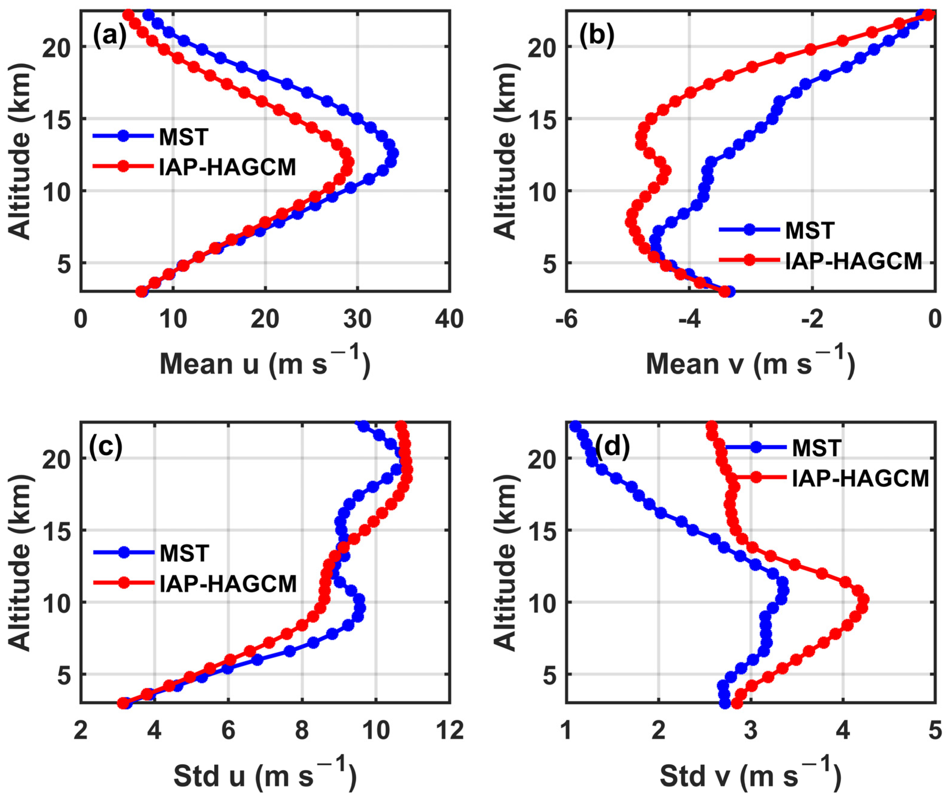
Figure 2 compares the IAP-HAGCM-computed mean winds and standard deviations at different altitudes with the corresponding Beijing MST radar observations from 2012 to 2014, for both the zonal and meridional components. As Figure 2a shows, the three-year-averaged zonal wind variation characteristics with altitude for the model simulations were consistent with the radar observations, exhibiting the maximum westerly wind speed at ~12 km. However, the model-simulated zonal wind was smaller than in the radar measurements within the altitudinal range of 7–20 km, and the difference was largest in the wind speed maximum altitude regions, which could reach ~5 m s−1. Above 20 km, the model results showed stronger easterly winds than those measured by the MST radar.
For the meridional wind (Figure 2b), it is evident that the IAP-HAGCM simulated a stronger yearly mean northerly wind than that observed by the radar within 3–22 km. The distribution characteristics of the model results and radar observations with altitude differed between 12 km and 15 km. The model results showed that the northerly wind speed first increased and then slightly decreased with altitude at 12–15 km, while it decreased with altitude for the MST radar observations.
For the standard deviation of zonal wind (Figure 2c), the model simulations were smaller than the MST radar observations below 12 km, and the opposite was true above 14 km. This indicates that the zonal wind simulated by the model is more discrete in the lower stratosphere than in the troposphere compared with the radar observations. The variation in the standard deviation of the meridional wind obtained from the model simulations and radar observations with altitude were similar. However, the values were larger for the IAP-HAGCM simulations than for the MST radar observations (Figure 2d).
Figure 3 shows the zonal and meridional winds obtained from the IAP-HAGCM and the MST radar measurements at 4.8 km, 12.0 km, and 20.4 km in different months during 2012–2014. It is apparent that the temporal distributions of zonal/meridional wind for the IAP-HAGCM and the MST radar are similar. The zonal and meridional winds showed the best agreement between model simulations and radar observations at the altitude of 4.8 km. However, it can be seen that at 12 km, where the westerly wind reached its maximum, the discrepancy between the IAP-HAGCM simulations and the MST radar observations was relatively larger than at other altitudes, especially for the meridional wind. The IAP-HAGCM also showed an interannual variability, as exhibited by the MST radar observations. Therefore, the IAP-HAGCM performs well in terms of the temporal distribution of horizontal winds in the troposphere and lower stratosphere. Nevertheless, more caution should be applied when using the model data at an altitude close to the westerly jet.

3.2. Statistical Analysis

Following on from the above comparisons and evaluations of the distribution and variations in horizontal wind with altitude and month, statistical analyses in the form of correlation coefficients, differences, and RMSE between the IAP-HAGCM simulations and MST radar observations were then carried out.

3.2.1. Correlation Coefficients

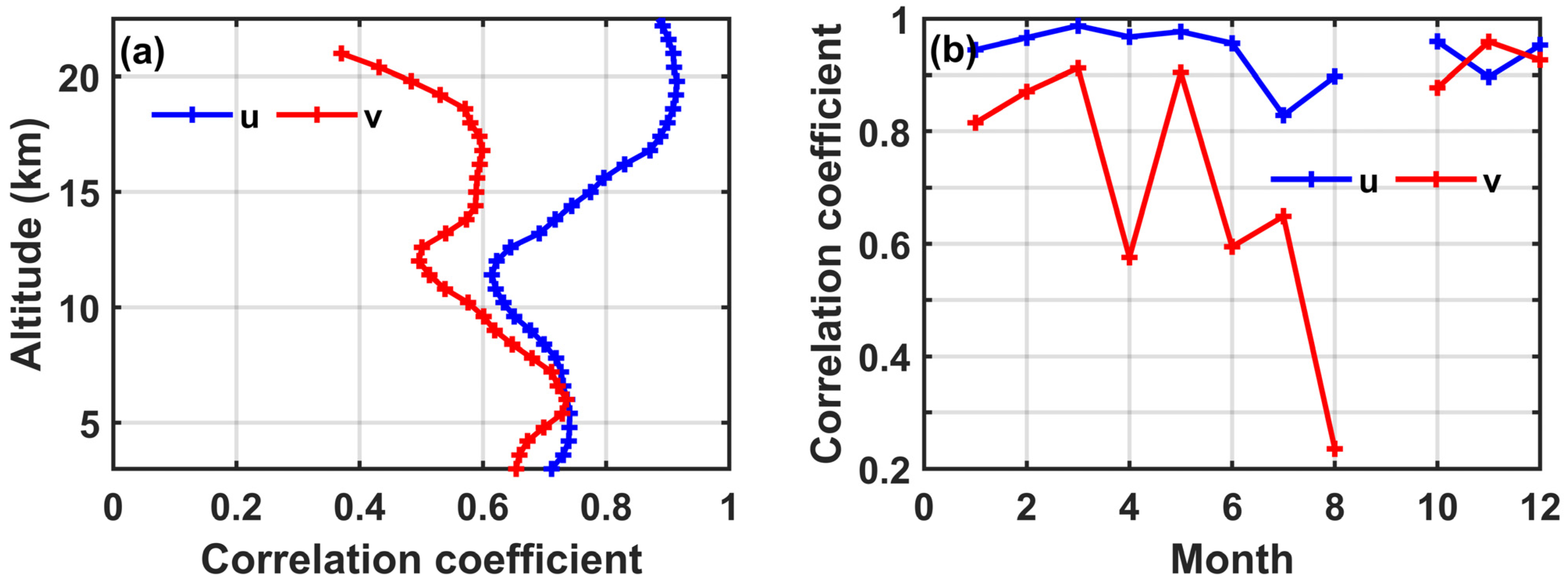
Figure 4 shows the variation in correlation coefficients of the zonal and meridional winds obtained from the IAP-HAGCM and the Beijing MST radar as a function of altitude and month. Overall, the correlation coefficients of the zonal wind were higher than those of the meridional wind. The linear fit of the model simulated and radar observed zonal (meridional) wind with 95% prediction interval were conducted, and the slope and intercept were 0.82 (0.80) and 0.87 (−1.49) m s−1, respectively.
As is seen in Figure 4a, the correlation coefficient shows two peaks at approximately 6 km and 18 km, and has a local minimum value at ~12 km for both the zonal and meridional wind. At an altitude above 15 km, the correlation coefficient of the zonal wind was between 0.80 and 0.92, increasing with altitude and beginning to decrease slightly over 20 km. However, the correlation coefficient of the meridional wind slightly increased within the altitudinal range of 14–17 km, and then decreased with altitude. The result was in accordance with the time–altitude distribution of the zonal and meridional winds in Figure 1, which suggests that, in the altitudinal range of 18–22.8 km, the temporal variation in the IAP-HAGCM zonal wind agreed well with that of the radar observations; however, this was not the case for the meridional wind.
Figure 4b shows that the correlation coefficients of the IAP-HAGCM and Beijing-MST-radar–obtained zonal wind were larger than 0.95 for all months apart from July, August, and November. As for the meridional winds, the correlation coefficients were larger than 0.9 in March, May, November, and December, while the value in August was lowest. The relatively low correlation coefficients for the zonal and meridional winds occurred in July and August, which is consistent with the reality that precipitation is mainly concentrated in these months in the area covered by the MST radar station. Therefore, it is inferred that in the months with a higher occurrence rate of mesoscale weather processes, the performance of the IAP-HAGCM-simulated horizontal wind is not as good as in other months.

3.2.2. Differences

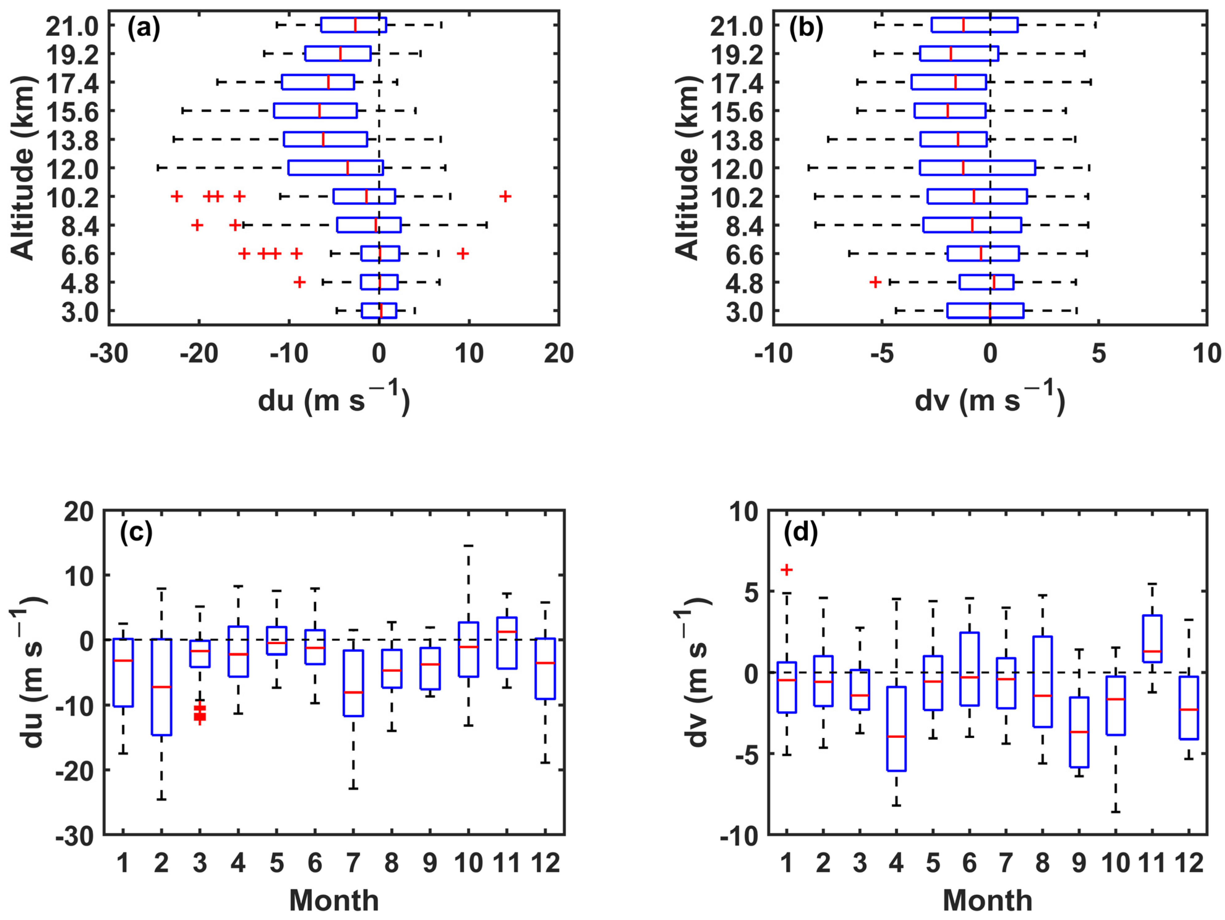
Figure 5 displays boxplots of the differences in zonal and meridional winds (du and dv) between the IAP-HAGCM and MST radar results in terms of altitude and month. As is shown in Figure 5a, the median value of du was approximately 0 m s−1 at 3–6.6 km, indicating that the model-simulated zonal wind is in good agreement with the radar observations in the lower troposphere. The median value of du between 8.4 km and 15.6 km decreased with altitude, which further indicates that the westerly wind speed simulated by the model is smaller than that observed by the MST radar, and the discrepancy is larger in this altitude region. Within the altitudinal range of 17.4 km to 21 km, the absolute median value of du decreased with increasing altitude. In the upper part of the westerly jet stream, from 12 to 15.6 km, the distribution of du was relatively more discrete. The median value of du within the altitudinal range of 3–21 km was distributed between −6.6 and 0 m s−1.
The absolute value of the median meridional wind difference also showed a pattern of increasing first and then decreasing with increasing altitude (Figure 5b). Like the zonal wind difference, dv reached a maximum value at 15.6 km. Unlike du, the discrete region of dv was distributed within the altitudinal range of 8.4–12 km, which was located in the lower part of the westerly jet. The median value of dv at 3–21 km was distributed between −2 and 0.2 m s−1.
The distribution of du from month to month showed apparent seasonal variations. As Figure 5c shows, there was significant deviation (model bias) in February and July, and good consistency in March, May and June. The larger deviation in February was mainly related to the weak intensity of the westerly jet simulated by the model. The larger deviation in July was mainly due to the fact that the intensity of the easterly wind simulated by the model was stronger than that observed by the MST radar in the lower stratosphere, as well as the simulated weaker westerly wind in the troposphere. Moreover, the easterly wind coverage simulated by the model was over 16 km, while it was over 18 km in the radar observations.
The absolute value of the meridional wind difference was larger in April and September than in other months, and the absolute median value was ~4 m s−1 (Figure 5d). The distribution of dv was relatively more discrete in April and August. November was the only month with a median difference greater than zero. The suggestion, therefore, is that more caution should be applied when using the simulated meridional wind data in April, August, September and November in the area represented by this comparison. The discrepancy in these months may be related to the local weather systems, which affect the atmospheric meridional circulation.

3.2.3. RMSE

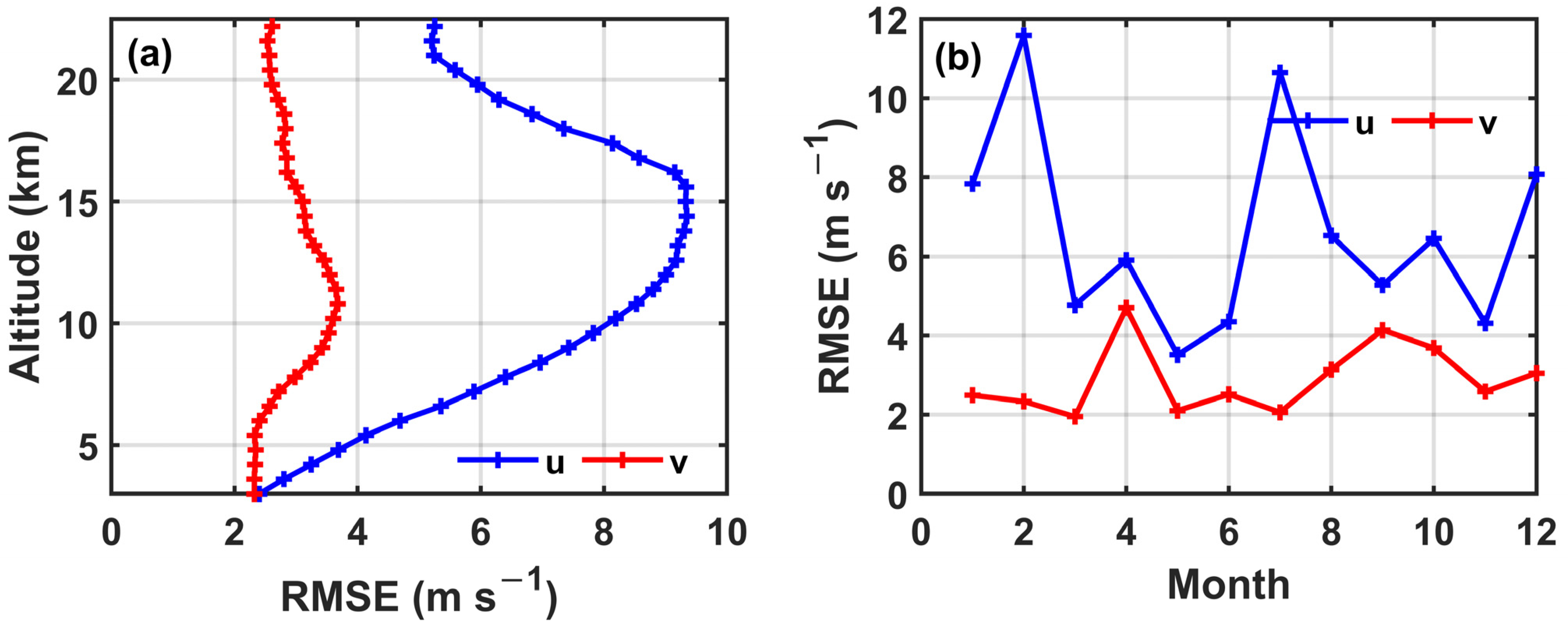
The distribution and variation in the RMSE between the IAP-HAGCM-simulated and MST-radar-observed zonal and meridional winds were investigated. The results are displayed in Figure 6.
As is shown in Figure 6a, the vertical distribution of the RMSE for the zonal and meridional components presents a peak at the altitudes of ~16 km and 12 km, respectively. Within the altitudinal range of 7–20 km, the RMSE of the zonal (meridional) wind ranged from 6 to 9.3 m s−1 (2.7 to 3.7 m s−1). It seems that, in the altitudinal region of the westerly jet and the transitional region of the troposphere and stratosphere, the discrepancy in horizontal wind between the model simulations and radar observations was relatively more significant.
The seasonal variation in the RMSE is presented in Figure 6b. For the zonal component, larger values were found in February and July, while they were smaller in the spring months. As for the meridional component, the value was highest in April and lower than 3 m s−1 in most months except September and October. It is suggested, therefore, that the horizontal wind discrepancy between the IAP-HAGCM simulations and Beijing MST radar observations in February, April, July and September is relatively larger. Thus, the simulated horizontal wind data in these months in the region covered by the Beijing MST radar should be used with caution.

3.3. Tides

Having evaluated the model’s ability to simulate the zonal and meridional winds, we further investigated the performance of IAP-HAGCM in simulating the diurnal and semidiurnal tides.

3.3.1. Diurnal Tides

Figure 7 shows the time–altitude cross-section of the zonal and meridional diurnal tidal amplitude obtained based on the horizontal wind of the IAP-HAGCM and the Beijing MST radar. It can be seen that the IAP-HAGCM reproduced the seasonality of the amplitudes and, partly, their vertical structures. The diurnal tidal amplitude time–altitude distribution pattern of the model looks similar to that of the MST radar observations. However, the IAP-HAGCM tends to underestimate the diurnal tidal amplitude for both the zonal and meridional component. The largest zonal diurnal tidal amplitudes were observed at ~10 km in April and reached values of 4–4.5 m s−1 (Figure 7c), while the maximum was ~5 m s−1 for the meridional component (Figure 7d). Nevertheless, the largest diurnal tidal amplitudes of the IAP-HAGCM ranged from 2.5 to 3 m s−1 for the meridional component (Figure 7b). Furthermore, the IAP-HAGCM meridional component exhibited larger amplitudes than the zonal diurnal tide, which was the same as that presented by the MST radar observations.

3.3.2. Semidiurnal Tides

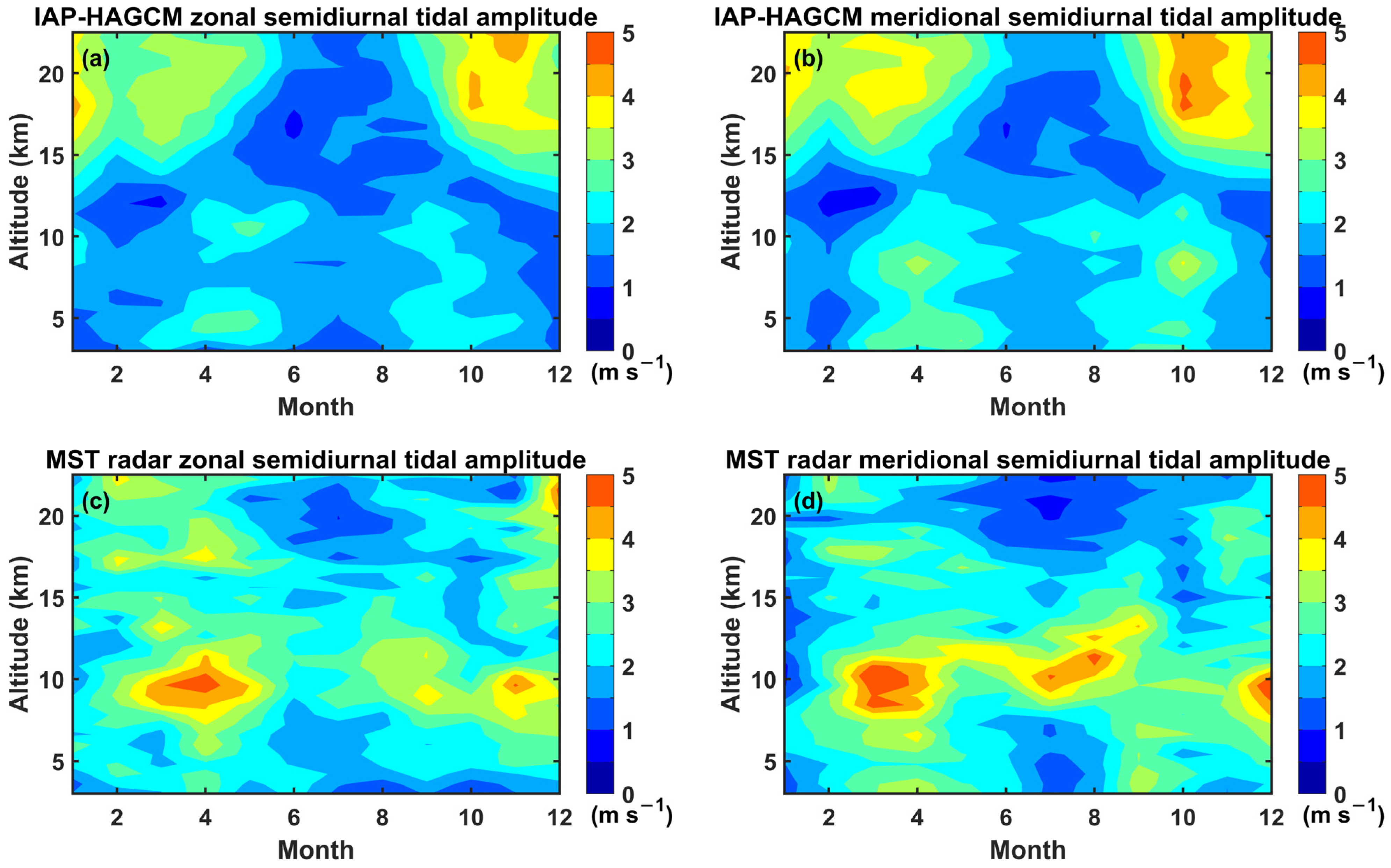
Figure 8 shows that the behavior of the seasonal amplitude for both the zonal and meridional semidiurnal tides was different between the model simulations and radar observations, especially at 8–12 km. For the IAP-HAGCM results, both the zonal and meridional semidiurnal tidal amplitudes were larger than those of the MST radar observations in all months apart from the summer months (JJA) at an altitude above 15 km. However, the IAP-HAGCM presented the zonal and meridional amplitude as almost the same, consistent with previous studies of semidiurnal tide amplitude characteristics in the mesosphere and lower thermosphere [22,64].
Furthermore, the semidiurnal tidal amplitude of IAP-HAGCM was comparable to that of the Beijing MST radar observations for both the zonal and meridional components. Moreover, both the model simulations and the radar observations exhibited a larger amplitude for the semidiurnal tide compared to that for the diurnal tide.

4. Discussion

The present paper evaluated the ability of the IAP-HAGCM to simulate horizontal winds in the troposphere and lower stratosphere, since the distribution and variation in these winds are essential for investigating atmospheric dynamic characteristics and processes. Additionally, certain information on GWs, tides, and planetary waves can also be extracted from the horizontal wind. Thus, if we know more details regarding the simulation ability of the IAP-HAGCM, such as in which altitudinal range and in which months it can reasonably represent the horizontal wind, then investigations based on simulations produced by the model can be more rigorous and reliable.
The present study sought to address the above question by comparing the zonal and meridional components of the horizontal winds obtained from the IAP-HAGCM simulations and MST radar observations. The MST radar data were evaluated by comparing them with the nearest radiosonde measurements, showing that the Beijing MST radar performs very well in obtaining high-quality horizontal wind data within the altitudinal range of 3–25 km [57]. One advantage of the MST radar is that it can not only observe the horizontal wind with high spatiotemporal resolution, but it can also work all day long under all weather conditions. Besides, the horizontal wind profile of the MST radar is obtained quasi-simultaneously and represents the atmospheric dynamic conditions above the radar site. In contrast, radiosonde data are obtained with the changing location of the balloon, and the temporal resolution is too coarse. Therefore, MST radar observation is an excellent option for evaluating the ability of the IAP-HAGCM to simulate the horizontal wind.

4.1. The Performance of the IAP-HAGCM in Simulating the Horizontal Wind Changes with Altitude, Season, and Month

According to the comparisons and investigations carried out in this study, the following key findings can be summarized:
  • The IAP-HAGCM reproduces a relatively reasonable altitude–month distribution of the zonal wind compared with Beijing MST radar observations, albeit the westerly wind velocity is underestimated and the easterly wind velocity is overestimated with a larger time–altitude region.
  • The consistency of the meridional wind between the IAP-HAGCM simulations and MST radar observations is not as good as it is for the zonal wind. This phenomenon has also been reported in previous studies, such as in a comparison of high-resolution regional model (WRF) wind outputs at Cochin from 315 m to 20 km with ST radar observations [65].
  • The IAP-HAGCM reproduces a similar temporal variation in the zonal and meridional components as exhibited by the radar observations, suggesting that the IAP-HAGCM-simulated horizontal winds can be used for analysis of the temporal variation.
  • In the lower troposphere, below 5 km, the horizontal winds obtained from the model and radar observations are in good agreement. However, larger discrepancies exist in the altitudinal range of the westerly jet’s location, as well as in the transition regions of the troposphere and stratosphere. The variation in the correlation coefficient, mean difference, and RMSE with altitude all show the above results.
  • The IAP-HAGCM can also simulate seasonal variation in horizontal wind similar to that observed by the radar. A larger discrepancy between the model simulations and radar observations can be found in certain months such as February and July for the zonal component, and April and September for the meridional component.
Table 2 shows the seasonal mean correlation coefficients, differences, and RMSE between the zonal and meridional winds obtained from the IAP-HAGCM and the Beijing MST radar. As can be seen, the correlation coefficient of the zonal wind was largest (lowest) in MAM (JJA), with a value of 0.98 (0.89) and 0.94 for ALL. As for the meridional wind, the correlation coefficient was lower in each season compared to the zonal component. The largest correlation coefficient was 0.84 in DJF, and the value was smallest in JJA (0.52). The absolute values of the seasonal mean difference were all smallest in SON for both the zonal and meridional component, and the mean values were −3.00 m s−1 and −0.70 m s−1 over the three years, respectively. The seasonal mean RMSE for the zonal (meridional) component was smallest in MAM (JJA), with a value of 4.73 m s−1 (2.57 m s−1), and the average RMSE over the three years was 6.60 m s−1 and 2.90 m s−1 for the zonal and meridional wind, respectively.

4.2. Possible Reasons

The reasons that the performance of the IAP-HAGCM-simulated horizontal wind varies with altitude and season can be explained in as follows: Firstly, it may be due to the characteristics and variability of the horizontal wind itself. For example, in the altitudinal range of the westerly jet, the discrepancy between different measurements or tools will increase for larger velocities and wind shears. Secondly, different weather systems dominate in different months and seasons. When meso–micro-scale weather systems occur frequently, the spatiotemporal variation in the atmospheric wind field is larger, the local circulation is complex, and the simulation performance of the model will be weakened. Thirdly, the model uses its unique parameterizations, such as the GW parameterization, which may not only affect the horizontal wind, but also change its spatial and temporal variation characteristics. For example, the effect of the GW parameterization on planetary waves is mainly in the winter hemisphere [66], which is seasonally dependent. As was shown by Ribstein et al. [67], the GW sources for the parameterizations seem be imposed at all altitudes, which is vertically dependent. Thus, disagreement between simulations and observations may occur at a certain altitude and/or in certain months, indicating that the impacts of physical parameterization schemes need be investigated in depth to address the uncertainties in simulating the horizontal wind. Additionally, in the previous evaluations of IAP-AGCMs mentioned above, the simulated subtropical westerly jets in both hemispheres were generally found to be overestimated, which is alleviated by the IAP-HAGCM. This may be due to the incorporation of non-orographic GW parameterizations, which can significantly reduce the systematic model bias of zonal-mean zonal wind, as indicated by Chun et al. [66].
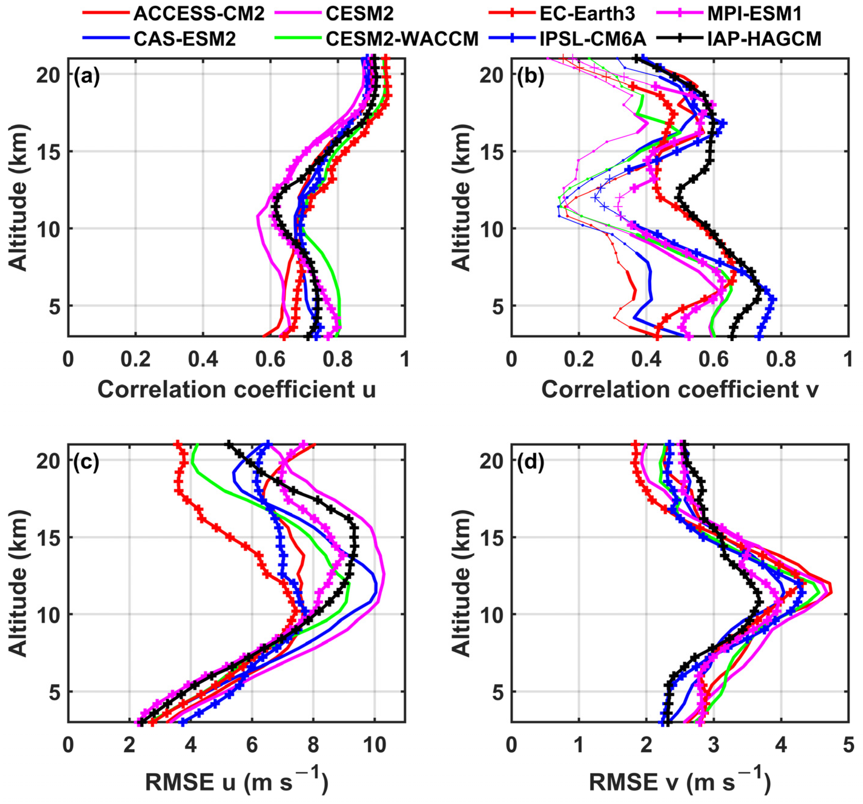
As a concise discussion regarding the potential physical mechanisms behind model bias, a comparison was made between the IAP-HAGCM and seven CMIP6 models (Table 3): CAS-ESM2-0 [35], CESM2 [68], ACCESS-CM2 [69], EC-Earth3 [70], IPSL-CM6A-LR [71], MPI-ESM1-2-LR [72], and CESM2-WACCM [68]. It is worth noting that these models have different atmospheric components since some coupled models share the same or similar atmospheric models. Among the seven models, CAS-ESM2-0 and CESM2 are classified as “low-top” models, with a model top reaching approximately 40 km. On the other hand, the remaining models are classified as “high-top” models, with a model top reaching approximately 80 km, except for CESM2-WACCM, which reaches approximately 130 km. The analysis focused on the AMIP monthly simulation results labeled “r1i1p1f1”, specifically examining the zonal wind, meridional wind, and geopotential height. The model grid data closest to the MST radar site (39.78°N, 116.95°E) was selected to conduct the analysis. More details regarding the CMIP6 models can be obtained from the CMIP6_CVs (https://wcrp-cmip.github.io/CMIP6_CVs/docs/CMIP6_source_id.html, accessed on 16 July 2023).
Many processes have an impact on the horizontal wind, and it is challenging to explain why a model performs better or worse. Since the tropospheric wind can be influenced by a combination of many complicated physics processes, such as convection, cloud microphysics, cloud macrophysics, planet boundary layer turbulence, orographic drag, and radiation transfer, IAP-HAGCM may exhibit a better representation of some of these processes below 10 km, as shown in Figure 9. It is worth noting that the IAP-HAGCM shows a better performance of the meridional wind simulations below 15 km (Figure 9b,d). In the stratosphere above 10 km, the interaction between waves and flow becomes more active, which can be influenced by model resolution and parameterized gravity waves. Although the IAP-HAGCM shares the same dynamical core with CAS-ESM2-0, it demonstrates superior simulation capabilities compared to CAS-ESM2-0, possibly due to its “high-top” and non-orographic gravity wave parameterizations. Similar behavior is expected between CESM2-WACCM and CESM2. EC-Earth3, which is based on the IFS of the ECMWF, exhibits an overall lower bias in the simulation of horizontal wind. This improved performance might be attributed to the extensive tuning of parameterizations and the adoption of Rayleigh friction to prevent unrealistically large winds [70]. In addition to physical parameterizations, the dynamic core of the model could play a crucial role in simulating horizontal winds. Several studies have highlighted the potential impact of the dynamical core on climate modeling [73,74], emphasizing the need for further investigations in the future.
The present study and its findings are essential for IAP-HAGCM users, who can take advantage of the model simulation results, and developers, who can improve the capabilities of the model. However, some limitations also exist. For instance, data from only one MST radar observatory were used in this study to partially evaluate the model’s simulation results. As such, it is necessary to use the observed data of several stations representative of various latitudes and longitudes to evaluate the model more comprehensively.

5. Conclusions

An assessment of the horizontal winds simulated by the IAP-HAGCM in the troposphere and lower stratosphere from 3 km to 22.8 km was conducted by comparing them with MST radar observations.
The existence of both agreement and discrepancy between the model simulations and radar observations at certain altitudes and in certain months, as summarized in the Discussion, suggests that model users should select the spatiotemporal regions with strong model simulation ability, according to their different research purposes.
For example, according to this study, the meridional and zonal winds produced by the IAP-HAGCM perform well when examined in terms of temporal variation. However, if one intends to study the atmospheric characteristics and processes in a specific month, it would be necessary to refer to the model evaluation results and avoid using them in the months with a larger deviation and/or significant discrete distribution of the difference between the model simulation and observations. Overall, the discrepancy is larger in the area of troposphere–stratosphere interaction and at altitudinal ranges with a larger wind speed, meaning more caution should be applied when using the model. In addition, the IAP-HAGCM has a differing ability in terms of reproducing the diurnal and semidiurnal tides. The model can effectively represent the spatial and temporal distribution characteristics of the diurnal tide amplitude, indicating that it has a good simulation ability from the perspective of diurnal variation characteristics.

Author Contributions

Conceptualization, Y.T. and Z.C. (Zhaoyang Chai); methodology, Y.T., Z.C. (Zhaoyang Chai) and Z.Y.; software, Y.T., Z.C. (Zhaoyang Chai) and Z.Y.; validation, Y.T., Z.C. (Zhaoyang Chai), Z.Y., Z.C. (Ze Chen) and J.J.; formal analysis, Y.T. and Z.C. (Zhaoyang Chai); investigation, Y.T., Z.C. (Zhaoyang Chai), Z.Y., Z.C. (Ze Chen) and J.J.; writing—original draft preparation, Y.T., Z.C. (Zhaoyang Chai) and Z.Y.; writing—review and editing, Y.T., Z.C. (Zhaoyang Chai), Z.Y., Z.C. (Ze Chen) and J.J.; visualization, Y.T. All authors have read and agreed to the published version of the manuscript.

Funding

This research was funded by the National Natural Science Foundation of China (Grant No. 41905042), the 14th Five-Year Plan Fundamental Research Funds of the Institute of Atmospheric Physics, Chinese Academy of Sciences (Grant No. E268021801), the Open Research Project of Large Research Infrastructures of Chinese Academy of Sciences—“Study on the interaction between low/mid-latitude atmosphere and ionosphere based on the Chinese Meridian Project”, the Open Research Project of State Key Laboratory of Tropical Oceanography, South China Sea Institute of Oceanology, Chinese Academy of Sciences (Project No. LTO2120), the Youth Innovation Promotion Association of CAS (2022074), and the National Key Scientific and Technological Infrastructure project “Earth System Numerical Simulation Facility” (EarthLab).

Institutional Review Board Statement

Not applicable.

Informed Consent Statement

Not applicable.

Data Availability Statement

Data related to this article are available upon request to the corresponding authors. CMIP6 data can be downloaded from the Earth System Grid Federation (https://esgf-node.llnl.gov/search/cmip6/, accessed on 16 July 2023).

Acknowledgments

We acknowledge the use of data from the Chinese Meridian Project. We sincerely thank all of the referees and editors for their constructive comments and suggestions.

Conflicts of Interest

The authors declare no conflict of interest.

References

  1. Fernando, H.J.S.; Mann, J.; Palma, J.M.L.M.; Lundquist, J.K.; Barthelmie, R.J.; Belo-Pereira, M.; Brown, W.O.J.; Chow, F.K.; Gerz, T.; Hocut, C.M.; et al. The Perdigao: Peering into Microscale Details of Mountain Winds. Bull. Am. Meteorol. Soc. 2019, 100, 799–820. [Google Scholar] [CrossRef]
  2. Simpson, C.C.; Sharples, J.J.; Evans, J.P. Sensitivity of atypical lateral fire spread to wind and slope. Geophys. Res. Lett. 2016, 43, 1744–1751. [Google Scholar] [CrossRef]
  3. Hoolohan, V.; Tomlin, A.S.; Cockerill, T. Improved near surface wind speed predictions using Gaussian process regression combined with numerical weather predictions and observed meteorological data. Renew. Energ. 2018, 126, 1043–1054. [Google Scholar] [CrossRef]
  4. Coccia, M. The effects of atmospheric stability with low wind speed and of air pollution on the accelerated transmission dynamics of COVID-19. Int. J. Environ. Stud. 2021, 78, 1–27. [Google Scholar] [CrossRef]
  5. Xing, W.; Sun, J.; Liu, H.; Xu, L. Numerical Simulation of the Local Circulation of Complex Topography on the Gaoligong Mountains. Chin. J. Atmos. Sci. 2021, 45, 746–758. [Google Scholar] [CrossRef]
  6. Su, Y.; Shi, C.; Mao, W.; Sun, S.; Xie, B.; Zhai, D. Hydrological Utility of CLDAS-Prcp Multi-source Fusion Precipitation Products in Qijiang River BasinTakingWRF-Hydro Model as an Example. Plateau Meteorol. 2022, 41, 617–629. [Google Scholar] [CrossRef]
  7. Zhang, C.; He, J.; Lai, X.; Liang, T.; Liu, Y.; Yang, W.; Che, H.; Gong, S. Impacts of High-Resolution Land Surface Data on Meteorological Field Simulation over Hainan. Plateau Meteorol. 2022, 41, 775–789. [Google Scholar] [CrossRef]
  8. Pan, L.L.; Liu, Y.B.; Roux, G.; Cheng, W.; Liu, Y.W.; Hu, J.; Jin, S.L.; Feng, S.L.; Du, J.; Peng, L.X. Seasonal variation of the surface wind forecast performance of the high-resolution WRF-RTFDDA system over China. Atmos. Res. 2021, 259, 105673. [Google Scholar] [CrossRef]
  9. Bao, J.W.; Michelson, S.A.; Persson, P.O.G.; Djalalova, I.V.; Wilczak, J.M. Observed and WRF-simulated low-level winds in a high-ozone episode during the Central California Ozone Study. J. Appl. Meterol. Clim. 2008, 47, 2372–2394. [Google Scholar] [CrossRef]
  10. Michelson, S.A.; Bao, J.W. Sensitivity of Low-Level Winds Simulated by the WRF Model in California’s Central Valley to Uncertainties in the Large-Scale Forcing and Soil Initialization. J. Appl. Meterol. Clim. 2008, 47, 3131–3149. [Google Scholar] [CrossRef]
  11. Fadnavis, S.; Deshpande, M.; Ghude, S.D.; Raj, P.E. Simulation of severe thunder storm event: A case study over Pune, India. Nat. Hazards 2014, 72, 927–943. [Google Scholar] [CrossRef]
  12. Boadh, R.; Satyanarayana, A.N.V.; Krishna, T.V.B.P.S.R.; Madala, S. Sensitivity of PBL schemes of the WRF-ARW model in simulating the boundary layer flow parameters for its application to air pollution dispersion modeling over a tropical station. Atmósfera 2016, 29, 61–81. [Google Scholar] [CrossRef] [Green Version]
  13. Kadaverugu, R.; Matli, C.; Biniwale, R. Suitability of WRF model for simulating meteorological variables in rural, semi-urban and urban environments of Central India. Meteorol. Atmos. Phys. 2021, 133, 1379–1393. [Google Scholar] [CrossRef]
  14. Xin, Y.F.; Rinke, A.; Bian, L.G.; Dethloff, K.; Xiao, C.D.; Mielke, M. Climate and Forecast Mode Simulations for Antarctica: Implications for Temperature and Wind. Adv. Atmos. Sci. 2010, 27, 1453–1472. [Google Scholar] [CrossRef]
  15. Bell, A. A Statistical Comparison of Radiosonde Observations to NCEP RCM3 Climate Model Atmospheric Wind Speed (Presentation). 2010. Available online: http://n2t.net/ark:/85065/d7n87cft (accessed on 16 July 2023).
  16. Weissmann, M.; Cardinali, C. Impact of airborne Doppler lidar observations on ECMWF forecasts. Q. J. Roy. Meteor. Soc. 2007, 133, 107–116. [Google Scholar] [CrossRef] [Green Version]
  17. Fritts, D.C.; Wang, D.-Y.; Blanchard, R.C. Gravity Wave and Tidal Structures between 60 and 140 km Inferred from Space Shuttle Reentry Data. J. Atmos. Sci. 1993, 50, 837–849. [Google Scholar] [CrossRef]
  18. Sun, L.; Lian, P.; Chang, X.; Yan, J. Near Space Atmosphere Modeling and its Effect on the Aircraft. Command. Control. Simul. 2016, 38, 107–111. [Google Scholar] [CrossRef]
  19. Cheng, X.; Xiao, C.; Hu, X. Research progress of the influence of atmospheric environment in near space on aerodynamic characteristics of hypersonic vehicles. Aerosp. Technol. 2018, 401, 22–28. [Google Scholar] [CrossRef]
  20. Wing, R.; Martic, M.; Triplett, C.; Hauchecorne, A.; Porteneuve, J.; Keckhut, P.; Courcoux, Y.; Yung, L.; Retailleau, P.; Cocuron, D. Gravity Wave Breaking Associated with Mesospheric Inversion Layers as Measured by the Ship-Borne BEM Monge Lidar and ICON-MIGHTI. Atmosphere 2021, 12, 1386. [Google Scholar] [CrossRef]
  21. Borchert, S.; Zhou, G.D.; Baldauf, M.; Schmidt, H.; Zangl, G.; Reinert, D. The upper-atmosphere extension of the ICON general circulation model (version: Ua-icon-1.0). Geosci. Model Dev. 2019, 12, 3541–3569. [Google Scholar] [CrossRef] [Green Version]
  22. Stober, G.; Kuchar, A.; Pokhotelov, D.; Liu, H.X.; Liu, H.L.; Schmidt, H.; Jacobi, C.; Baumgarten, K.; Brown, P.; Janches, D.; et al. Interhemispheric differences of mesosphere-lower thermosphere winds and tides investigated from three whole-atmosphere models and meteor radar observations. Atmos. Chem. Phys. 2021, 21, 13855–13902. [Google Scholar] [CrossRef]
  23. Wilks, D.S. Chapter 9—Forecast Verification. In Statistical Methods in the Atmospheric Sciences, 4th ed.; Wilks, D.S., Ed.; Elsevier: Amsterdam, The Netherlands, 2019; pp. 369–483. [Google Scholar] [CrossRef]
  24. Gunwani, P.; Mohan, M. Sensitivity of WRF model estimates to various PBL parameterizations in different climatic zones over India. Atmos. Res. 2017, 194, 43–65. [Google Scholar] [CrossRef]
  25. Guo, J.P.; Liu, B.M.; Gong, W.; Shi, L.J.; Zhang, Y.; Ma, Y.Y.; Zhang, J.; Chen, T.M.; Bai, K.X.; Stoffelen, A.; et al. Technical note: First comparison of wind observations from ESA’s satellite mission Aeolus and ground-based radar wind profiler network of China. Atmos. Chem. Phys. 2021, 21, 2945–2958. [Google Scholar] [CrossRef]
  26. Munoz, L.E.; Campozano, L.V.; Guevara, D.C.; Parra, R.; Tonato, D.; Suntaxi, A.; Maisincho, L.; Paez, C.; Villacis, M.; Cordova, J.; et al. Comparison of Radiosonde Measurements of Meteorological Variables with Drone, Satellite Products, and WRF Simulations in the Tropical Andes: The Case of Quito, Ecuador. Atmosphere 2023, 14, 264. [Google Scholar] [CrossRef]
  27. Zhou, B.; Xue, X.; Yi, W.; Ye, H.; Zeng, J.; Chen, J.; Wu, J.; Chen, T.; Dou, X. A comparison of MLT wind between meteor radar chain data and SDWACCM results. Earth Planet. Phys. 2022, 6, 451–464. [Google Scholar] [CrossRef]
  28. Liu, Y.J.; Wei, Z.G.; Chen, G.Y.; Liu, Y.J.; Zhu, X.; Zheng, Z.Y. Shift of the Arctic polar vortex in recent decades and its simulation by the NCEP CFSv2. Phys. Chem. Earth 2020, 115, 102823. [Google Scholar] [CrossRef]
  29. Richter, J.H.; Garcia, R.R. On the forcing of the Mesospheric Semi-Annual Oscillation in the whole atmosphere community climate model. Geophys. Res. Lett. 2006, 33, L01806. [Google Scholar] [CrossRef]
  30. Hamilton, K.; Hertzog, A.; Vial, F.; Stenchikov, G. Longitudinal variation of the stratospheric quasi-biennial oscillation. J. Atmos. Sci. 2004, 61, 383–402. [Google Scholar] [CrossRef]
  31. Butchart, N.; Anstey, J.A.; Hamilton, K.; Osprey, S.; McLandress, C.; Bushell, A.C.; Kawatani, Y.; Kim, Y.H.; Lott, F.; Scinocca, J.; et al. Overview of experiment design and comparison of models participating in phase 1 of the SPARC Quasi-Biennial Oscillation initiative (QBOi). Geosci. Model Dev. 2018, 11, 1009–1032. [Google Scholar] [CrossRef] [Green Version]
  32. Chai, Z.; Zhang, M.; Zeng, Q.; Xie, J.; You, T.; Zhang, H. Simulation of the QBO in IAP-AGCM: Analysis of momentum budget. Atmos. Oceanic Sci. Lett. 2021, 14, 100021. [Google Scholar] [CrossRef]
  33. Zeng, Q.; Zhang, X.; Liang, X.; Yuan, C.; Chen, S. Documentation of IAP two-level atmospheric general circulation model. USDo Energy 1989, 383, 90143–90145. [Google Scholar]
  34. Zhang, X. Dynamical framework of IAP nine-level atmospheric general circulation model. Adv. Atmos. Sci. 1990, 7, 67–77. [Google Scholar] [CrossRef]
  35. Zhang, H.; Zhang, M.H.; Jin, J.B.; Fei, K.C.; Ji, D.Y.; Wu, C.L.; Zhu, J.W.; He, J.X.; Chai, Z.Y.; Xie, J.B.; et al. Description and Climate Simulation Performance of CAS-ESM Version 2. J. Adv. Model. Earth Syst. 2020, 12, e2020MS002210. [Google Scholar] [CrossRef]
  36. Zuo, R.; Zeng, Q.; Zhang, M. A Numerical Simulation of Monsoon and the Correlation Between Monsoon and Westerlies. Chin. J. Atmos. Sci. 2004, 28, 7–22. [Google Scholar] [CrossRef]
  37. Zhang, H.; Zhang, M.H.; Zeng, Q.C. Sensitivity of Simulated Climate to Two Atmospheric Models: Interpretation of Differences between Dry Models and Moist Models. Mon. Weather Rev. 2013, 141, 1558–1576. [Google Scholar] [CrossRef]
  38. Bi, X. An Improved Nine-Level Atmospheric General Circulation Model and Its Application to Climate Simulation. Ph.D. Thesis, Institute of Atmospheric Physics, Chinese Academy of Sciences, Beijing, China, 1993. [Google Scholar]
  39. Liang, X. Description of a nine-level grid point atmospheric general circulation model. Adv. Atmos. Sci. 1996, 13, 269–298. [Google Scholar] [CrossRef]
  40. Zuo, R. Development of New Generation Grid Point Atmospheric General Circulation Model with High Resolution. Ph.D. Thesis, China People’s Liberation Army University of Science and Technology, Changsha, China, 2003. [Google Scholar]
  41. Zhang, H.; Lin, Z.; Zeng, Q. The Computational Scheme and the Test for Dynamical Framework of IAP AGCM-4. Chin. J. Atmos. Sci. 2009, 33, 1267–1285. [Google Scholar] [CrossRef]
  42. Zhang, H. Development of IAP Atmospheric General Circulation Model Version 4.0 and Its Climate Simulations. Ph.D. Thesis, Institute of Atmospheric Physics, Chinese Academy of Sciences, Bejing, China, 2009. [Google Scholar]
  43. Chai, Z.; Zhang, M.; Zeng, Q.; Zhang, H.; Jin, J.; Xie, J.; You, T. A high-top version of IAP-AGCM: Preliminary assessment and sensitivity IAP-AGCM. Atmos. Oceanic Sci. Lett. 2021, 14, 100025. [Google Scholar] [CrossRef]
  44. Xue, F.; Bi, X.Q.; Lin, Y.H. Modelling the global monsoon system by IAP 9L AGCM. Adv. Atmos. Sci. 2001, 18, 404–412. [Google Scholar] [CrossRef]
  45. Zuo, R.; Zhang, M.; Zhang, D.; Wang, A.; Zeng, Q. Designing and Climatic Numerical Modeling of 21-Level AGCM (IAP AGCM-Ⅲ) Part Ⅰ. Dynamical Framework. Chin. J. Atmos. Sci. 2004, 28, 659–674. [Google Scholar] [CrossRef]
  46. Sun, H.; Zhou, G.; Zeng, Q. Assessments of the Climate System Model (CAS-ESM-C) Using IAP AGCM4 as Its Atmospheric Component. Chin. J. Atmos. Sci. 2012, 36, 215–233. [Google Scholar] [CrossRef]
  47. Richter, J.H.; Sassi, F.; Garcia, R.R. Toward a Physically Based Gravity Wave Source Parameterization in a General Circulation Model. J. Atmos. Sci. 2010, 67, 136–156. [Google Scholar] [CrossRef]
  48. Lindzen, R.S. On the Development of the Theory of the Qbo. Bull. Am. Meteorol. Soc. 1987, 68, 329–337. [Google Scholar] [CrossRef]
  49. Mcfarlane, N.A. The Effect of Orographically Excited Gravity-Wave Drag on the General-Circulation of the Lower Stratosphere and Troposphere. J. Atmos. Sci. 1987, 44, 1775–1800. [Google Scholar] [CrossRef]
  50. Beres, J.H.; Alexander, M.J.; Holton, J.R. A method of specifying the gravity wave spectrum above convection based on latent heating properties and background wind. J. Atmos. Sci. 2004, 61, 324–337. [Google Scholar] [CrossRef]
  51. Beres, J.H.; Garcia, R.R.; Boville, B.A.; Sassi, F. Implementation of a gravity wave source spectrum parameterization dependent on the properties of convection in the Whole Atmosphere Community Climate Model (WACCM). J. Geophys. Res.-Atmos. 2005, 110. [Google Scholar] [CrossRef] [Green Version]
  52. Zhang, G.J.; Mcfarlane, N.A. Sensitivity of Climate Simulations to the Parameterization of Cumulus Convection in the Canadian Climate Center General-Circulation Model. Atmos. Ocean 1995, 33, 407–446. [Google Scholar] [CrossRef] [Green Version]
  53. Richter, J.H.; Solomon, A.; Bacmeister, J.T. On the simulation of the quasi-biennial oscillation in the Community Atmosphere Model, version 5. J. Geophys. Res. Atmos. 2014, 119, 3045–3062. [Google Scholar] [CrossRef]
  54. Taylor, K.E.; Stouffer, R.J.; Meehl, G.A. An Overview of Cmip5 and the Experiment Design. Bull. Am. Meteorol. Soc. 2012, 93, 485–498. [Google Scholar] [CrossRef] [Green Version]
  55. Wang, C.; Xu, J.; Lu, D.; Yue, X.; Xue, X.; Chen, G.; Yan, J.; Yan, Y.; Lan, A.; Wang, J.; et al. Construction Progress of Chinese Meridian Project Phase II. Chin. J. Atmos. Sci. 2022, 42, 539–545. [Google Scholar] [CrossRef]
  56. Tian, Y.F.; Lu, D.R. Preliminary analysis of Beijing MST radar observation results in the mesosphere-lower thermosphere. Chin. J. Geophys. 2016, 59, 440–452. [Google Scholar] [CrossRef]
  57. Tian, Y.F.; Lu, D.R. Comparison of Beijing MST radar and radiosonde horizontal wind measurements. Adv. Atmos. Sci. 2017, 34, 39–53. [Google Scholar] [CrossRef]
  58. Tian, Y.; Chen, Z.; Lyu, D. A dataset of Beijing MST radar horizontal wind fields at Xianghe Station in 2012. China Sci. Data 2021, 6, 1. [Google Scholar] [CrossRef]
  59. Chen, F.L.; Chen, G.; Shi, C.H.; Tian, Y.F.; Zhang, S.D.; Huang, K.M. Strong downdrafts preceding rapid tropopause ascent and their potential to identify cross-tropopause stratospheric intrusions. Ann. Geophys. 2018, 36, 1403–1417. [Google Scholar] [CrossRef] [Green Version]
  60. Chen, F.L.; Chen, G.; Tian, Y.F.; Zhang, S.D.; Huang, K.M.; Wu, C.; Zhang, W.F. High-resolution Beijing mesosphere-stratosphere-troposphere (MST) radar detection of tropopause structure and variability over Xianghe (39.75 degrees N, 116.96 degrees E), China. Ann. Geophys. 2019, 37, 631–643. [Google Scholar] [CrossRef] [Green Version]
  61. Chen, Z.; Tian, Y.F.; Lue, D.R. Turbulence Parameters in the Troposphere-Lower Stratosphere Observed by Beijing MST Radar. Remote Sens. 2022, 14, 947. [Google Scholar] [CrossRef]
  62. Chen, Z.; Tian, Y.F.; Wang, Y.A.; Bi, Y.H.; Wu, X.; Huo, J.; Pan, L.J.; Wang, Y.; Lu, D.R. Turbulence parameters measured by the Beijing mesosphere-stratosphere-troposphere radar in the troposphere and lower stratosphere with three models: Comparison and analyses. Atmos. Meas. Tech. 2022, 15, 4785–4800. [Google Scholar] [CrossRef]
  63. Chen, Z.; Tian, Y.; Lu, D. Improving the Processing Algorithm of Beijing MST Radar Power Spectral Density Data. J. Appl. Meterol. Sci. 2020, 31, 694–705. [Google Scholar] [CrossRef]
  64. Jacobi, C. 6 year mean prevailing winds and tides measured by VHF meteor radar over Collm (51.3 degrees N, 13.0 degrees E). J. Atmos. Solar-Terr. Phys. 2012, 78–79, 8–18. [Google Scholar] [CrossRef]
  65. Sivan, C.; Rakesh, V.; Abhilash, S.; Mohanakumar, K. Evaluation of global reanalysis winds and high-resolution regional model outputs with the 205 MHz stratosphere-troposphere wind profiler radar observations. Q. J. Roy. Meteor. Soc. 2021, 147, 2562–2579. [Google Scholar] [CrossRef]
  66. Chun, H.Y.; Song, I.S.; Baik, J.J.; Kim, Y.J. Impact of a convectively forced gravity wave drag parameterization in NCAR CCM3. J. Clim. 2004, 17, 3530–3547. [Google Scholar] [CrossRef]
  67. Ribstein, B.; Millet, C.; Lott, F.; de la Camara, A. Can We Improve the Realism of Gravity Wave Parameterizations by Imposing Sources at All Altitudes in the Atmosphere? J. Adv. Model. Earth Syst. 2022, 14, e2021MS002563. [Google Scholar] [CrossRef]
  68. Danabasoglu, G.; Lamarque, J.-F.; Bacmeister, J.; Bailey, D.A.; DuVivier, A.K.; Edwards, J.; Emmons, L.K.; Fasullo, J.; Garcia, R.; Gettelman, A.; et al. The Community Earth System Model Version 2 (CESM2). J. Adv. Model. Earth Syst. 2020, 12, e2019MS001916. [Google Scholar] [CrossRef] [Green Version]
  69. Bi, D.; Dix, M.; Marsland, S.; O’Farrell, S.; Sullivan, A.; Bodman, R.; Law, R.; Harman, I.; Srbinovsky, J.; Rashid, H.A.; et al. Configuration and spin-up of ACCESS-CM2, the new generation Australian Community Climate and Earth System Simulator Coupled Model. J. South. Hemisph. Earth Syst. Sci. 2020, 70, 225–251. [Google Scholar] [CrossRef]
  70. Döscher, R.; Acosta, M.; Alessandri, A.; Anthoni, P.; Arsouze, T.; Bergman, T.; Bernardello, R.; Boussetta, S.; Caron, L.P.; Carver, G.; et al. The EC-Earth3 Earth system model for the Coupled Model Intercomparison Project 6. Geosci. Model Dev. 2022, 15, 2973–3020. [Google Scholar] [CrossRef]
  71. Boucher, O.; Servonnat, J.; Albright, A.L.; Aumont, O.; Balkanski, Y.; Bastrikov, V.; Bekki, S.; Bonnet, R.; Bony, S.; Bopp, L.; et al. Presentation and Evaluation of the IPSL-CM6A-LR Climate Model. J. Adv. Model. Earth Syst. 2020, 12, e2019MS002010. [Google Scholar] [CrossRef]
  72. Mauritsen, T.; Bader, J.; Becker, T.; Behrens, J.; Bittner, M.; Brokopf, R.; Brovkin, V.; Claussen, M.; Crueger, T.; Esch, M.; et al. Developments in the MPI-M Earth System Model version 1.2 (MPI-ESM1.2) and Its Response to Increasing CO2. J. Adv. Model. Earth Syst. 2019, 11, 998–1038. [Google Scholar] [CrossRef] [Green Version]
  73. Jun, S.-Y.; Choi, S.-J.; Kim, B.-M. Dynamical Core in Atmospheric Model Does Matter in the Simulation of Arctic Climate. Geophys. Res. Lett. 2018, 45, 2805–2814. [Google Scholar] [CrossRef]
  74. Hall, D.M.; Ullrich, P.A.; Reed, K.A.; Jablonowski, C.; Nair, R.D.; Tufo, H.M. Dynamical Core Model Intercomparison Project (DCMIP) tracer transport test results for CAM-SE. Q. J. Roy. Meteor. Soc. 2016, 142, 1672–1684. [Google Scholar] [CrossRef]
Figure 1. Comparison of the monthly mean (a,b) zonal and (c,d) meridional wind in a composite year between (a,c) the IAP-HAGCM simulations and (b,d) MST radar observations.
Remotesensing 15 03571 g001
Figure 2. The (a,b) mean and (c,d) standard deviation profiles of the (a,c) zonal and (b,d) meridional wind of the IAP-HAGCM simulations (red) and MST radar observations (blue).
Remotesensing 15 03571 g002
Figure 3. The variation in (a,c,e) zonal and (b,d,f) meridional winds obtained from the IAP-HAGCM simulations (red) and MST radar observations (blue) during 2012–2014 at the altitude of (a,b) 4.8 km, (c,d) 12.0 km, and (e,f) 20.4 km.
Remotesensing 15 03571 g003
Figure 4. The (a) vertical distribution and (b) monthly variation in the correlation coefficients of the IAP-HAGCM-simulated and MST-radar-observed zonal (red) and meridional (blue) winds. The results passed the significance test with a 95% confidence interval.
Remotesensing 15 03571 g004
Figure 5. Boxplots of the (a,c) zonal and (b,d) meridional wind differences between the IAP-HAGCM-simulated and MST-radar-observed results in terms of (a,b) altitude and (c,d) month, with the minimum, 25% quartile, median (the red −), 75% quartile, maximum values, and outliers (the red +) shown.
Remotesensing 15 03571 g005
Figure 6. The (a) vertical distribution and (b) monthly variation in the RMSE between the IAP-HAGCM-simulated and MST-radar-observed zonal (blue) and meridional (red) winds.
Remotesensing 15 03571 g006
Figure 7. Time–altitude cross-sections of the (a,c) zonal and (b,d) meridional diurnal tidal amplitude calculated based on the horizontal winds obtained from the (a,b) IAP-HAGCM simulation and (c,d) Beijing MST radar observations.
Remotesensing 15 03571 g007
Figure 8. Time–altitude cross-sections of the (a,c) zonal and (b,d) meridional semidiurnal tidal amplitude calculated based on the horizontal winds obtained from the (a,b) IAP-HAGCM simulation and (c,d) Beijing MST radar observations.
Remotesensing 15 03571 g008
Figure 9. The vertical distribution of the correlation coefficient of the IAP-HAGCM together with the other seven CMIP6-model-simulated and MST-radar-observed zonal (a) and meridional (b) winds; (c,d) are the same as (a,b) but for the RMSE between the model simulations and the radar observations. The light-colored thin curves in (b) indicate that the significance test with 95% confidence level was not passed, while the thick curves in (a,b) show the results have passed the significance test.
Remotesensing 15 03571 g009
Table 1. The development of the IAP-AGCM.
VersionVertical LevelsModel TopHorizontal Resolution
IAP-AGCM1 [33]2200 hPa4° × 5°
IAP-AGCM2 [34,38,39]910 hPa4° × 5°
IAP-AGCM3 [40]2110 hPa2° × 2.5°
IAP-AGCM4 [41,42]262.3 hPa1.4° × 1.4°
IAP-AGCM5 [35]352.3 hPa1.4° × 1.4°
Table 2. The seasonal mean correlation coefficients (Ru and Rv), differences (du and dv), and RMSE (RMSEu and RMSEv) for the zonal and meridional winds obtained from the IAP-HAGCM and the Beijing MST radar. MAM: averaged for March, April, and May; JJA: averaged for June, July, and August; SON: averaged for September, October, and November; DJF: averaged for December, January, and February; ALL: averaged for all months of the three years, i.e., the annual mean.
MAMJJASONDJFALL
Ru0.980.890.930.950.94
Rv0.800.520.780.840.73
du−1.20−4.77−0.68−4.87−3.00
dv−1.35−0.41−0.29−0.67−0.70
RMSEu4.737.175.359.166.60
RMSEv2.92 2.57 3.472.632.90
Table 3. CMIP6 models selected to be compared with the IAP-HAGCM. ATM, atmospheric component; NGWD, non-orographic gravity wave drag.
Source_idATMModel Top (Levels)Horizontal
Resolution
Dynamical CoreNGWD
ACCESS-CM2UM10.6 GA7.185 km (85)1.25° × 1.875°ENDGame non-hydrostatic schemeYes
CAS-ESM2-0IAP-AGCM5.040 km (35)1.4° × 1.4°IAP finite difference schemeNo
CESM2CAM640 km (32)0.9° × 1.25°Finite volume schemeNo
CESM2-WACCMWACCM6130 km (70)0.9° × 1.25°Finite volume schemeYes
EC-Earth3IFS cy36r480 km (91)T255 (80 km)Spectral transform method and finite element schemeYes
IPSL-CM6A-LRLMDZ 6A-LR80 km (79)2.5° × 1.3°Finite difference schemeYes
MPI-ESM1-2-LRECHAM6.380 km (47)T63 (200 km)Spectral transform methodYes
Disclaimer/Publisher’s Note: The statements, opinions and data contained in all publications are solely those of the individual author(s) and contributor(s) and not of MDPI and/or the editor(s). MDPI and/or the editor(s) disclaim responsibility for any injury to people or property resulting from any ideas, methods, instructions or products referred to in the content.