Article

A New Spatio-Temporal Selection Method for Estimating Upwelling Medium-Wave Radiation

1
School of Science, RMIT University, Melbourne 3001, Australia
2
Faculty of Geo-Information Science and Earth Observation (ITC), University of Twente, 7500AA Enschede, The Netherlands
3
Bushfire and Natural Hazards Co-Operative Research Centre, East Melbourne 3005, Australia
4
School of Geography, Planning and Spatial Sciences, University of Tasmania, Hobart 7015, Australia
*
Author to whom correspondence should be addressed.
Remote Sens. 2023, 15(14), 3521; https://doi.org/10.3390/rs15143521
Submission received: 2 June 2023 / Revised: 5 July 2023 / Accepted: 11 July 2023 / Published: 12 July 2023

Abstract

:
Accurate estimates of the unperturbed state of upwelling radiation from the earth’s surface are vital to the detection and classification of anomalous radiation values. Determining radiative anomalies in the landscape is critical for isolating change, a key application being wildfire detection, which is reliant upon knowledge of a location’s radiation budget sans fire. Most techniques for deriving the unperturbed background state of a location use that location’s spatial context, that is, the pixels immediately surrounding the target. Spatial contextual estimation can be subject to error due to occlusion of the pixel’s spatial context and issues such as land cover heterogeneity. This paper proposes a new method of deriving background radiation levels by decoupling the set of prediction pixels used for estimation from the target location in a Spatio-Temporal Selection (STS) process. The process selects training pixels for predictive purposes from a target-centred search area based on their similarity with the target pixel in terms of brightness temperature over a prescribed time period. The proposed STS process was applied to images from the AHI-8 geostationary sensor centred over the Asia-Pacific, and comparisons were made to both brightness temperature estimates from the spatial context and to sensor measurements. This comparison showed that the STS method provided between 10–40% reduction in estimation error over the commonly utilised contextual estimator; in addition, the STS method increased the availability of estimates in comparison to the spatial context by between 12–31%. Image reconstruction using the method resulted in high-fidelity reproductions of the examined landscape, with standing geographic features and areas experiencing thermal anomalies readily identifiable on the resulting images.

Graphical Abstract

1. Introduction

Remote sensing is a powerful tool that is often used to investigate changes in the landscape over time, and has been employed in this way across applications such as vegetation change [1], urban growth [2], and disaster response [3] among other change-related applications. The mapping of change in the physical environment requires knowledge of the state of the landscape pre-change in order to determine the nature and magnitude of such changes [4]. In an ideal case, change tracking would make use of data that span the temporal domain as well as the spatial domain. With knowledge about how the earth’s surface reacts to nominal physical phenomena over time, predictions can be made about a landscape’s expected behaviour at a subsequent point in time. This information can then be leveraged to provide a method of isolating and identifying anomalous landscape-level behaviour while identifying obscuring influences such as cloud, smoke, and fire by comparing a predicted image to data recorded “in reality”.
Fire detection is a well established application of remote sensing, with many commonly used products produced from both low-earth orbit and geostationary sensors [5,6,7,8]. The most important element of the electromagnetic spectrum for these purposes is the Medium-Wave InfraRed (MWIR) (3 μ m –4 μ m ), where the peak emissions from fire energy sources occurs. Excess radiation at this wavelength allows fire to be detected even when it constitutes only a small portion of an image segment (down to 10 5 of a pixel) [9]. Estimating upwelling radiation at this wavelength is complicated by the dual-source nature of electromagnetic energy, with components made up of both thermal emission and solar reflection [10].
Geostationary imagers have been used for several decades now as a source of remote sensing data encompassing all kinds of atmospheric and surface phenomena, and in particular are ideal for supplementing higher resolution images from low earth orbiting sensors. With newer generation satellites such as JAXA’s Himawari 8 and 9 satellites and the GOES-16 and GOES-17 satellites in the western hemisphere, a significant increase in temporal resolution is now available from sensors of this type, with AHI-8/9 measuring the full disk at 10 min intervals. In the fire detection space, a number of studies have focused on adapting existing algorithms, predominantly using background brightness temperature derived from the image context [11,12,13,14,15]. The work of [15,16] utilised this extra temporal resolution to provide single-pixel fitting of the diurnal temperature cycle in an extension of the method developed by [17]; however, this method continues to present shortcomings with regard to cloud masking techniques, which had not been refined for the sensor in question at the time. As for leveraging data in both the temporal and spatial realms, only [18] have presented a method in this space. Their method uses the mean of temperature for the entire area of study as an estimator of brightness temperature difference over a time period, neglecting the difference of response to solar radiation that many types of land cover display at a per-pixel level.
Fire detection algorithms such as those in [5] rely on the difference between the candidate fire pixel and a reference background value. In the majority of algorithms, this reference value is derived from a convolution-style filtering approach, where values from surrounding pixels are averaged to provide the temperature estimate. A comprehensive examination of this practice was undertaken in [19] that highlighted shortcomings in the use of such a method, especially in areas of high spatial frequency (i.e., heterogeneous landscapes). The aforementioned study showed that the contextual derivation of temperature acted in a manner similar to an edge detector in areas exhibiting spatial fragmentation, not unlike the moving window analysis in [20], which resulted in increased errors in temperature estimation. These areas are often of vital importance for fire detection purposes, with wildland-urban interfaces being the areas as most risk from the impacts of wildfire [21].
The practice of using convolution filtering for estimation of MWIR background radiation is based on the spatial autocorrelation effect, where areas near a specific location are assumed to exhibit characteristics more similar to that location than those further away [22]. The top-of-atmosphere solar radiation component of an upward-welling signal strongly adheres to similar behaviour due to its strong relationship with the angles of the solar azimuth and zenith [4]. Surface characteristics such as the slope and aspect of a surface, land cover type, and water bodies can all affect the signal emanating from a pixel. However, in areas where human activity has created fragmentation in a landscape, the relative uniformity found in untouched landscapes means that this is less likely to hold true [20]. In many cases, the likelihood is high that areas exist outside of the immediate proximity of a target pixel that could more comprehensively characterise the signal of a location than those nearer by.
Considering that the typical phenomena that can obscure upward-welling signals from candidate pixels (e.g., fire) display a high level of spatial autocorrelation themselves, and are more likely to influence areas proximal to a potential target, the availability of a method that is less reliant on the local area for estimating radiation may provide greater robustness in reaching a solution. The present study seeks to introduce a new method of brightness temperature estimation in the MWIR called the Spatio-Temporal Selection (STS) method; this method is based on the determination of pixel locations that more closely resemble the MWIR behaviour of the target pixel within a defined local region. For this paper, (Section 2) describes how the proposed method tracks the history of brightness temperatures for a given period, selects training pixels based on their statistical fit to the target pixel, and makes predictions for brightness temperature based on values from a prediction image. Section 3 assesses the proposed method’s validity against the common estimation method. Finally, Section 4 examines the results obtained using the proposed method and discusses its potential for improving image reproduction for other purposes.

2. Materials and Methods

This section describes the implementation of the proposed method on the selected dataset (Section 2.1) followed by a formal description (Section 2.2) clarifying the main framework of the method and outlining the parameters that can be modified for refinement of solutions.

2.1. Test Data Example

For this study, data from the Japan Meteorological Agency’s AHI-8 sensor on the Himawari-8 geostationary satellite was used. This satellite, positioned in geostationary orbit at 140.7 °E longitude, provides coverage over eastern Asia, the western Pacific, and Australia with a 16-band multispectral imager (three visible light, three near infrared, one medium-wave infrared, and nine thermal infrared bands) [23]. While the main purpose of the sensor is for meteorological forecasting, the high temporal resolution (full disk recorded every 10 min ) has encouraged use of the imagery for detection and monitoring of rapid change in the environment. Images captured from AHI’s MWIR Band 7 ( 3.7   μ m ) were masked for removal of water pixels using the ancillary land–sea masks supplied by the Australian Bureau of Meteorology. A cloud mask was applied to the images from this band as well, based on the mask applied to AHI-8 outlined in [24], which was itself adopted from a similar mask applied to GOES imagery [25].
To facilitate the study, a number of 200 × 200 pixel case study areas were identified across the AHI full disk, which are detailed in Table 1 and shown in Figure 1. These areas underwent an analysis of fire activity for the year 2016 using the VNP14IMGML VIIRS active fire product [26], with the peak of fire activity in a 30 day rolling window over the year adopted as the central day of a 31 day period of examination. These case study areas were then divided into 50 × 50 pixel regions; areas that mainly consisted of sea pixels were dismissed, and from the remaining areas seven 50 × 50 regions were randomly selected for analysis. The times selected for making pixel predictions were at the local times corresponding to 09:00, 12:00, 15:00, and midnight, with a random offset of 0, 10, 20, 30, 40, or 50 min added to provide statistical independence for overlapping training sets. The selected study areas covered approximately 18.5   M h a of land in total.
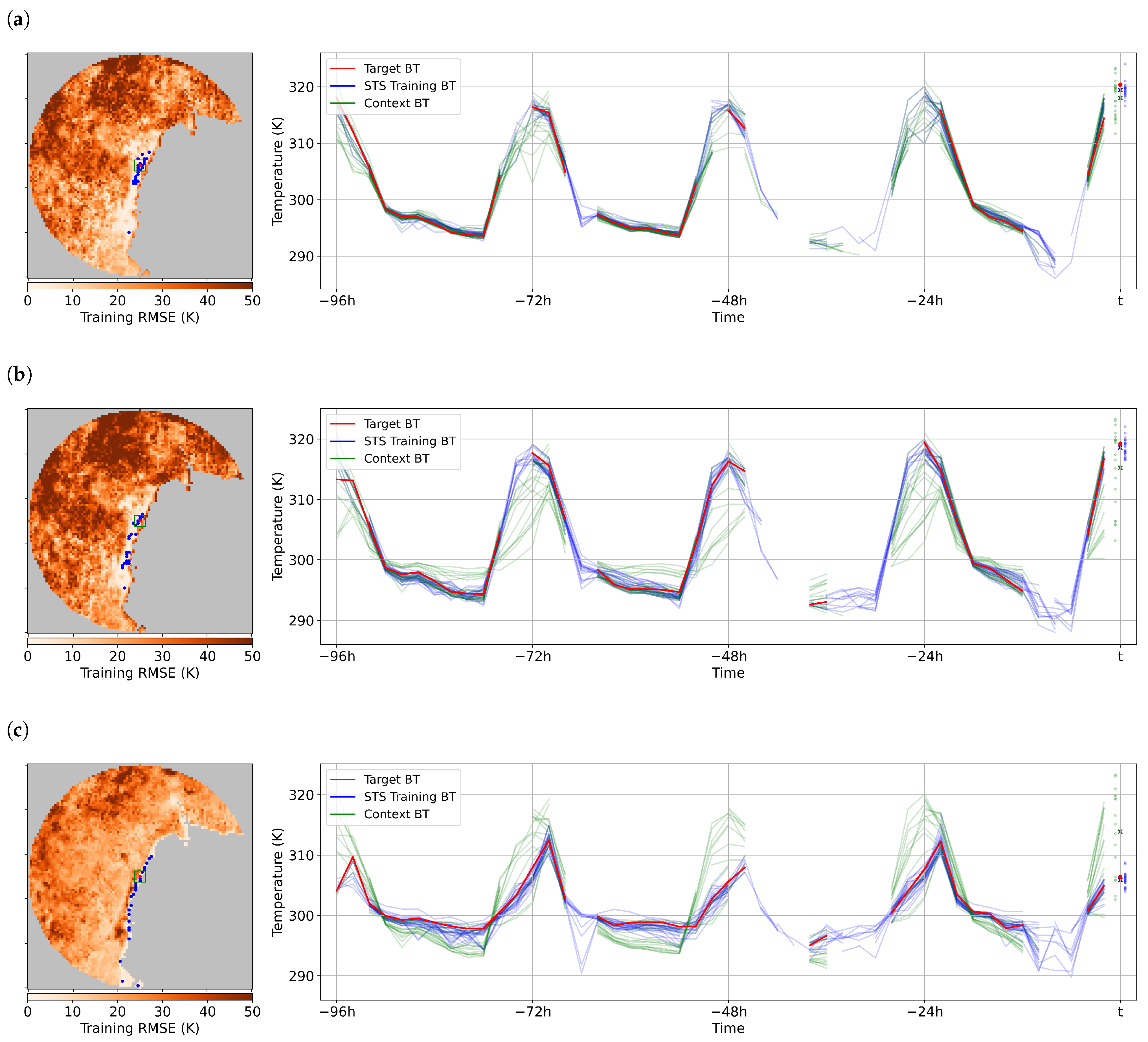
The procedure for providing training data for image reconstruction was to select a circular area 50 pixels in radius surrounding each of the target pixels in the region, stack the previous 48 images together at intervals of two hours, and calculate the difference between all image pixels within this radius and the target over all images. A root mean square error (RMSE) was then calculated from all of the resulting temperature differences in the training set of images, as shown in the left-hand images in Figure 2. Any training locations that had less than four coincident observations with the target over the 48 images were deemed to have insufficient data to determine correlation, and were eliminated from further analysis. From the remaining potential training locations, the RMSEs were sorted and the 24 locations with the lowest error compared to the target were selected for the prediction phase, as shown in the right-hand images in Figure 2. In the prediction step, a minimum of six training locations had to be available in order to provide an STS estimate of brightness temperature; target locations with less than six were discarded from the analysis. The unmasked values of the training locations from the image at the time of prediction were then filtered for outliers (removal of ± 2 σ ) and the remaining values at the training locations were averaged for the final estimation of temperature at the target location.
Comparisons of brightness temperatures for analysis purposes were undertaken where the solutions for STS estimation and contextual estimation were coincident with the raw brightness temperature from the prediction image. Contextual estimates were calculated based on the guidelines for computational accuracy set out in [19], in which it was determined that 5 × 5 contextual estimates with at least 65% of adjacent pixel availability represents the minimum required to ensure contextual estimation accuracy.

2.2. Formal Description

Figure 3 demonstrates the STS method from first principles. Important variables for altering the method’s implementation depending upon the conditions of use are as follows:
  • n i m a g e —number of images in the pixel training stack
  • ν —time gap between images in the pixel training stack
  • r t r a i n —the radius of restraint when searching for training pixels around a target pixel
  • c—the total number of coincident measurements between potential training pixels and the target in the training stack
  • n t r a i n —the number of training pixels selected for use in target estimation
  • λ —the time period starting from prediction stack creation during which training selections remain valid.
By altering these parameters from those set in this study, a number of improvements in the derived solution may be possible. For instance, n i m a g e sets the number of images over which to assess the validity of training pixels. Generally, a larger number of assessed images is better when judging training suitability; however, this could be traded off for a larger search radius to maintain processing efficiency. Furthermore, n i m a g e is closely related to the value of ν . In this study, values of 48 images and two hours, respectively, were selected for these parameters in order to find a balance of measurements over the diurnal cycle of the training area. The alteration of these values to affect training accuracy is related to the cloud conditions in the training area during a given predictive assessment. Lengthening the time over which pixels are assessed for suitability can help to mitigate the presence of weather systems and their associated cloud cover, although it may not account for major alterations to a landscape such as those caused by fire or flooding events. Training should occur over a range of diurnal conditions in order to mitigate the effects of developing convective clouds, which are a constant feature observed in certain assessed landscapes during the afternoon daytime period.
The values of r t r a i n and n t r a i n speak to the suitability of the area surrounding the target for providing sufficient training data. The search radius r t r a i n should be increased or decreased dependent upon the likelihood of correct characterisation, noting that in certain cases (such as in Figure 2c) suitable pixels may not display the typical spatial autocorrelation pattern usually associated with temperature estimation. Increasing the number of selected training pixels may improve the likelihood of obtaining a valid estimation, especially in cloudy prediction images, although it is likely to result in less accurate estimation when the prediction image is clear, as the extra values for the target estimation are drawn from pixel values that are less correlated. The c value set in this process relates to the expected accuracy of predictor pixels; setting this value too low may result in the selection of training pixels that are highly correlated for a very short portion of the training stack and that otherwise have very little in common, whereas setting it too high may reduce the effectiveness of the training pixel search, especially if the number of values approaches the number of valid measurements of the target pixel over the training period.

2.3. Overall Accuracy Assessment

The typical method of assessing accuracy is based on the variation in estimations made from the recorded values. While this is a sensible approach to a perfect landscape with no occluding features, the inclusion of comparisons to anomalous temperature values from the imagery, whether from fire activity or misattributed cloud, can lead to this type of assessment being flawed. A situation where obvious image contamination has occurred penalises the accuracy of any estimation method that is able to correctly identify an error, with the level of penalty increasing with the effectiveness of the error identification. As such, the accuracy results for this study are provided both with and without these anomalous values in order to allow for better comparison with previous studies. Upon visual examination of the images, an anomaly rate of 2% was adopted as the standard level of error in the brightness temperature images required in order to not penalise the accurate identification of these errors.
Two sets of accuracy assessment figures are presented in the results: a comparison between the STS and context estimates on the one hand and the image temperatures on the other, with and without the largest 2% of anomalous differences from the image temperatures as measured in absolute terms. The mean and standard deviations of the differences of the two methods from the image temperature are both reported, along with the percentage difference between the methods in terms of the standard deviation.

3. Results

3.1. Training Pixel Selection

Figure 2 displays a typical set of training data selections and subsequent estimations for a number of closely located target pixels near the east coast of Kalimantan. The maps to the left of this figure depict the RMSEs of each of the potential training pixels relative to the target, with lighter colours in areas that appear more like the target pixel. In the depicted cases, there is an obvious trend whereby noise values increase with the distance from the target pixel, which is not unexpected behaviour. Of interest here is the propensity of training pixel selection to occur in areas of similar land use, especially with regard to land–water interfaces. In Figure 2a, lower RMSEs occur in the strip of land immediately inland from the coast. This area is heavily cleared and contains more urban areas in comparison to other parts of this region. The second pixel selected more heavily favours this area, and the selected training pixels stretch out along the coastal fringe. The pixel depicted in Figure 2c is coastal in nature, and the low RMSEs of the training pixels reflect this. Accordingly, the pixels selected for training purposes by STS are strung out in a line along the coast, reflecting this characterisation.
The right half of Figure 2 shows the various pixel trajectories over the STS training period. The red target value is compared to the temperature values of all pixels in the training set; however, only the pixels selected for fitting and the pixels describing the 5 × 5 area surrounding the target are shown here. Figure 2a has the least noisy contextual temperature estimation shown here, with most disagreement between the target and the context values occurring in the middle of the day. The blue training values tend to stick closer to the target, with mild deviations mostly in the night-time period, where at times no comparison takes place. The adjacent contextual values at time t t are shown in green, whereas temperatures from the STS training group are shown in blue. In this case, the range of values seen in the contextual pixels is around 7 K larger, with the contextual mean approximately 5 K below the target figure. The blue STS pixels are more closely grouped, with the mean value of the STS solution far closer to the recorded value. In this case, the STS training set shares nine pixels with the contextual surrounds of the target, with the values obtained from pixels outside of this region strengthening the resulting solution.
The two figures in Figure 2b,c show more extreme examples of potential pixel trajectories from a highly variable landscape. The contextual pixel values shown in Figure 2b again show the most variation during the day, while demonstrating some variation during the night. This type of lagging temperature variation is a hallmark of coastal locations where, the pixels are often a mixture of land and water; the water portion of these pixels tends to retain heat during the night in comparison to the adjacent land areas, and during the day the reduced reflection coupled with the delay in heating of the water compared to the land areas results in the peak brightness temperatures occurring later in the day. Using the selected STS pixels reduces the effect on the estimation of values from pixels with temporal lag, again with a tighter grouping of brightness temperature values and fewer low-value outliers. Figure 2c depicts the fitting of a coastal pixel, showing the lagging of the STS pixel values compared to the higher temperatures from the contextual surroundings. Thus, the resulting set of pixel values on which estimates can be based is much more tightly grouped in the case of STS, with the resulting mean estimates providing a decrease in the estimation error of 15 K compared to the contextual estimate. Considering the appearance of the pixel trajectories in this case, it is likely that the attributed error in the contextual method in this region is permanent in nature, with seasonality and tidal effects being the major contributing factors to potential variation in this error.
It should be noted that for contextual estimation purposes the three pixels highlighted in this figure have a high amount of contextual overlap. Not only does this figure show the improvement in the statistical fitting of the target brightness temperature over the fitting period, it demonstrates the likely variation of contextually derived temperatures over the course of the diurnal cycle, with pixels such as those in Figure 2c suffering from consistent positive anomalies during the night and negative anomalies throughout the day. These effects are heightened by increased spatial heterogeneity in the contextual envelope of a pixel, and are likely to trigger simple threshold anomaly detectors if not screened for.

3.2. Overall Accuracy Assessment

Table 2 describes the errors and standard deviations of the two assessed estimation methods against the measured brightness temperature values for each case study area. Biases in both methods tend to be fairly low, with all but one study area having mean differences of less than 0.1 K. Increases in the means of the STS estimation tend to be due to the omission error of the cloud mask used, which drives estimates from STS lower due to the prevalence of misattributed cloud. The four study areas showing the most improvement in variation were thl, chn, jpn, and sea, with decreases in estimate variation of between 19–34% in the dataset including anomalies. Of particular note is the improvement in estimate error in the chn study area, where contextual estimation performs significantly better than in the other areas covered.
Temperature estimation using the STS method remains a challenge in the bor and sib case study areas, with increases in the variation of estimates of 19–34%, respectively. Errors with STS estimation in these areas are generally caused by the large amount of cloud occlusion present in these image sets, both with regard to the training period, which causes mis-selection of training pixels, and in the prediction image, where cloud values reduce the number of training pixels that can contribute to a solution for a target.
The error rates for the estimates reported with the anomalous temperatures removed shows a decrease in variance for both estimation methods, with a 10–17% drop in contextual estimation error and a 16–28% drop in STS estimation error. On the whole, the elimination of outliers treats the remaining STS variations favourably, with an decrease in comparison to the contextual estimates across all sites. The selection of the 2% anomaly rate seems to be supported by these numbers, although decreases in reported variance were much lower in the jpn area than in others due to a much higher rate of anomalous temperature differences resulting from the extreme heterogenity of the landscape. If this dataset with the outliers removed is assumed to provide a better account of temperature estimation for the bulk of temperature values, then the temperature characterisation is improving by up to 40% when using the STS method in favourable conditions.

3.3. Image Assessment

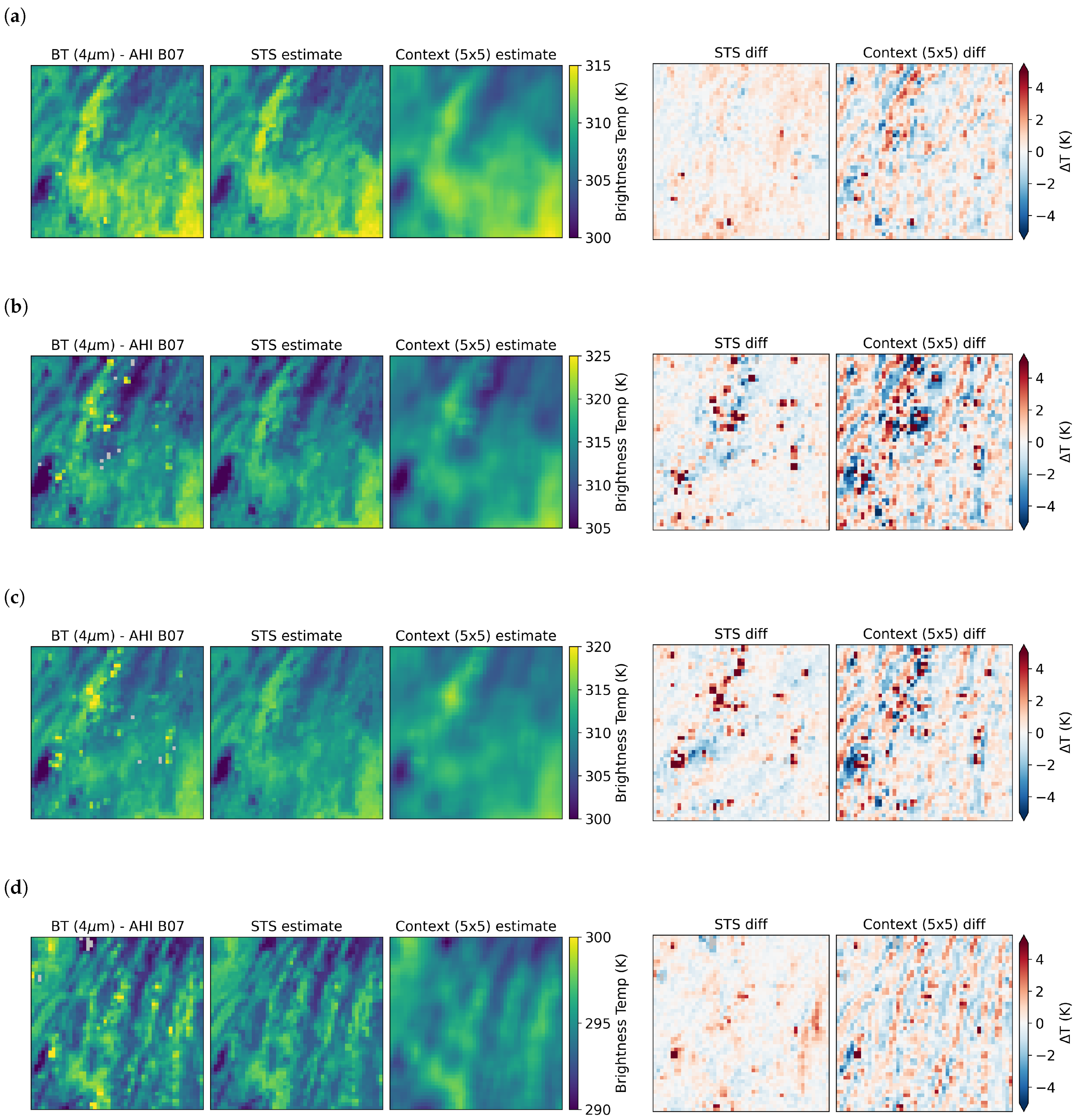
Figure 4 shows a series of images that demonstrate the STS and contextual methods over a subset of the thl region. The area shown is centred over the Loei province of northern Thailand, with the northern half of the image over western Laos. From left to right, the images show the brightness temperature image from AHI Band 7, the STS estimation of the region, and the contextual estimation of the region. The two rightmost images show the differences between the first image and the second and third images, respectively, providing an overall assessment of the temperature differences. At first glance, in Figure 4a there appears to be a marked similarity in the landscape depiction produced by STS in comparison to the sensor image. Fine details in the image are retained; for instance, the silhouette of the Mekong River shown in the upper centre of the brightness temperature image is evident in the STS estimation, as is the stratification of temperature zones in the north and west part of the region. In contrast, the contextual image performs as more of a smoothing filter, reducing the overall contrast of the image and dulling the finer details of temperature change. These effects can be seen most markedly in the difference images, with an overall decrease in both the high and low temperature magnitudes seen on the STS difference image compared to the equivalent image for the contextual approach. Despite the overall lowering of temperature variation, the STS method is able to identify anomalous pixels in the original image, for instance in the west and south of the STS difference image.
The increased error experienced at the midday period can be seen in Figure 4b, which shows the result of an estimation at noon local time. A marked feature of this particular image time is a number of anomalies shown in the STS difference image in the area. The large number of red pixels, which may signify agricultural burning in the area, are easy to identify on the STS difference image; however, in the contextual difference image they tend to become mixed with the landscape edge effects. One notable effect of these high temperature anomalies in the contextual difference image is the subsequent effect these higher temperatures have on estimation at the edge of the anomalies. The high temperatures tend to result in a ring of low-temperature results surrounding this activity. Generally, fire detection algorithms remove this problem by flagging the fire pixels as anomalous before estimating surrounding temperatures; however, as these treatments vary widely in application and effectiveness, an evaluation of such methods is beyond the scope of this study. Figure 4c,d shows the subsequent progression of the temperatures in the area through the afternoon and into the next night. Although landscape patterns seen during the day tend to change at night due to differences in surface emissivity and subsequent heat retention/loss, the STS estimation method has no issue with maintaining image reproduction quality even with changes in the distribution of temperature gradients. Anomalous temperature activity in this area continues throughout the night; although contextual estimation highlights anomalies more strongly at night, it provides a far noisier solution for pixels that are not undergoing anomalous activity.

3.4. Estimation Availability

Table 3 shows a breakdown of the availability of estimations using the STS and context methods against the recorded brightness temperatures from images. The first two columns of the table respectively report the total amount of land pixels assessed from the seven 50 × 50 sub-regions from each case study area for the 124 images of the assessment period and the number of pixels that recorded a brightness temperature value after the cloud mask was applied. As assessed by the cloud mask, cloud was least prevalent in the thl and nwa areas and most prevalent in the jpn and sib areas, with more than half of all pixels in the latter areas affected by cloud. Contextual estimation can occur in 90–97% of cases where brightness temperature values exist, which is a higher rate of estimates than reported in [19]; however, this rate is highly dependent on the identification of cloud, which is in turn dependent on the cloud mask used. When using the STS training selection process, the diversity of the sampling area means that estimation can take place in more fragmented images where contextual estimation may not be possible. Of course, due to the buffer of 50 pixels applied to each temperature estimation process in this study, the area that can be potentially sampled is far higher than for contextual temperature estimation; however, if it is assumed that the average cloud conditions over the buffered area and the assessed area are similar, the STS method provides estimates of temperature in around 20% more cases than the brightness temperature images themselves. It is beyond the scope of this study to assess the accuracy of the extra pixels provided by the STS method, mainly due to the lack of direct comparison to recorded image pixels; however, these instances could be used to validate whether or not the masking technique by which pixels are being eliminated from examination (in this case, the cloud mask) is working effectively.

4. Discussion

With regard to parameter selection for STS in this study, it is important to note that only one set of parameters was examined, which affects the results obtained from the STS estimation in a number of ways. The training of pixels in this instance occurred over the preceding 48 images at a two hour spacing, for a total training period of 96 h. Training accuracy is reliant on variation in the pixels gathered through the time series in order to filter out less accurate prediction pixels; significant periods of cloud during this training process lead to a reduction in coinciding measurements between the target and ideal prediction pixels within the search radius. This weakness to cloud cover during the training period can be mitigated by varying the time between training images, as lengthening the time between images results lessened influence of weather effects in the short term. Here, care must be taken to ensure that training happens within a reasonable period before the prediction step, as changes to the landscape increase the error for these pixels when attempting to find matches. An opportunity to shorten the time step exists if there is a known period of clear sky before the prediction step. A fuller reckoning of the method’s accuracy when altering the time step is required in order to make recommendations regarding these effects. Another opportunity afforded by the STS method in estimation of temperatures is the ability to select persistent training pixels, which can assist in periods where training data are less accurate. Training pixel locations can be held fixed over subsequent prediction steps if the noise in the nearer-term time series of predictors is too great; this represents another interesting potential topic for investigation.
It is less certain whether the other parameters set in this implementation of STS require further iteration. The number of training pixels set for prediction was fixed at 24 in this instance, which was done to provide a direct comparison to the number of pixels usually available for contextual estimation. The pixels selected in the training step are the available pixels most similar to the target; thus, adding extra training pixels adds extra robustness to estimation in the face of cloud cover in the prediction image while adding extra noise to the solution in more favourable conditions. The likelihood is high that users will prefer the most robust solutions on cloudy days, though the exact number of training pixels required to supply this requires further examination. The radius of prediction set in this study generally resulted in an accurate set of training pixels for estimation in most cases, with notable exceptions being coastal and urban areas and where major landscape change occurred during the training period. Locations such as these may benefit from a wider range of pixels to provide training data, although it should be noted that increasing the search radius involves a quadratic leap in processing time. Areas displaying these temperature behaviours may be better served by a concerted classification scheme in order to identify ideal training pixels outside of the search bounds without unduly increasing a search radius that is adequate for most solutions.
With regard to the range of contextual variation shown here in comparison to the results reported in [19], selection of the time of day of images analysed is an important consideration; the previous study selected only one time point during the day, whereas the predictions in this study were made at four time points over one diurnal cycle. Notwithstanding this difference, the values calculated by contextual estimation agree well with those in the previous study, apart from decreases in variation in the jpn area and increases in variation in the bor and sib areas. As noted in Section 2.1, contextual assessment was restricted to an evaluation of a 5 × 5 window, as described in [19], with only estimates based upon 65% contextual availability being used. This is the best case scenario for contextual estimation; as can be seen in the left panels of Figure 2a–c, introduction of areas in increasingly larger contextual windows leads to increased variation in both the training data selected and the subsequent temperature estimation.
In general, use of the STS method for estimation results in a 20–30% improvement in global variation of brightness temperatures, with the most notable improvement of up to 40% for the Thailand site. In the field of fire detection and monitoring, considering the increasing focus on detection of smaller fires earlier in their life, the use of a more stable estimator for brightness temperature can assist in the reduction and refinement of fire detection thresholds. Considering the nature of the STS implementation here, there may be room for significant improvement in temperature estimation beyond those figures. Susceptibility to cloud cover remains a major concern, as with any method of background estimation. The cloud mask used in this study seemed to have trouble with omission errors in the case study areas, causing cloud-affected brightness temperature values to slip through and skew the training evaluation. These errors can affect both the training data (by eliminating more accurate training pixels from the selection) and the target pixel itself (as temperature errors caused by cloud hamper the comparison of all pixels to the target). These target errors can lead to mis-selection of training pixels that share the same errors at the same times instead of more accurate selection candidates. While the periods of high cloud cover experienced in the Borneo and Siberia study areas may not explain all of the errors that occurred in these locations, the extra cloud cover and the poor performance of the cloud mask used in this study suggest that significantly improved performance in areas such as these may be as simple as adopting a more appropriate cloud product.
The comparison sets used in this study only focused on areas where brightness temperature from the original AHI image and estimations from both the contextual and STS methods were available. This omitted the portion of pixels that achieved an STS estimate with sufficient robustness while lacking a coincident contextual estimation. The threshold set in this study for contextual availability stemmed from a study by [19] which concluded that 65% of available adjacent pixels was the minimum for achieving sufficient accuracy in estimation. As the error in STS estimation is similarly related to the number of available predictors, and is not adjacency-based, it is possible that some or all of the STS pixel estimations outside the valid contextual area may have been healthy estimates of temperature, which could have led to wider extensibility of this estimator for anomaly detection compared to the contextual method.
Notwithstanding the issues with cloud cover demonstrated in this study, one potential adjustment to the STS that could make cloud less of a factor could be internal implementation of a cloud masking procedure. In a clear sky state, the STS process has been shown to provide highly accurate background predictions and has demonstrated the ability to pick out misattributed cloud (see Figure 5c). With enough confidence in estimations from a clear period, anomalous predictor pixels in a prediction set could be flagged as such, and estimations within the same image could avoid using these marked training pixels. This could feed into an updated training image for use in subsequent prediction activity further on in time. There are limits to the effectiveness of such a process, as a persistent period of bad weather may break the continuity of cloud propagation through the training series, and the demonstrated issues with landscape change during the training period may not be adequately addressed by such an approach. Nevertheless, such an extension, if made to work, could further enhance the results of this estimation method.
While this study primarily focused on the application of the proposed method to geostationary satellite imagery, there is scope for introducing such a system for improving the selection of temperature estimators in low earth orbiting imagery. For instance, to provide an example based upon VIIRS imagery, which has a daytime equator crossing time of approximately 1330 local time, STS fitting for geostationary pixels could be provided based on images for a number of days previous. As diurnal variation is less of a concern when providing a fit for specific time periods, allowing for the natural variation in sun-synchronous capture times from orbital variation, STS estimation could focus on images captured at ±50 min from the converted local time of the pixel instead of the full diurnal cycle examined in this paper. The fitting and identification of training locations in the geostationary imagery could then provide “search areas” for examining pixels from previous VIIRS captures, which are of course captured at a higher spatial resolution, from which a number of suitable training pixels could be identified for fitting on the active VIIRS image. Considering the reduced scale that the geostationary sensors capture at, STS selections in this application are likely to provide fitting data that are much further away from the target pixel than regular contextual estimation (even in expanding window mode); however, this may lead to increased robustness in temperature estimation, as localised factors that affect temperature estimation such as image IFOV bleeding, weather, and fire are eliminated.
Further examination of the STS method in action can provide insight into common artifacts seen in contextual temperature estimation while highlighting problems that need additional attention. Examples such as areas of low-temperature anomalies around high-temperature anomalies (Figure 5a), high-temperature anomalies engulfed by neighbouring anomalous values (Figure 5b), low-temperature anomalies suffering similar treatment (Figure 5c), and standing anomalies such as urban heat islands (Figure 5d) all demonstrate the instability of using contextual temperature estimation in proximity to anomalous behaviour. While it should be noted that most contextual estimation techniques in the fire detection space eliminate wildly anomalous adjacent pixel values before providing an estimation, this relies on assumptions about the nature of the anomalies being detected, including thresholding techniques that essentially constitute a minimum detectable fire size. Anomaly detection using contextual estimation is reliant on high contrast between the thermal target and its surroundings; in cases where a thermal anomaly is close to a pixel boundary, spreads over multiple tiles, or where the spread function of the imager in question leads to mixing of the target area with the surroundings when calculating values, selection of training data from non-adjacent locations can add to the robustness of brightness temperature estimation, especially during the earliest point of fire activity when its emitted energy is the lowest.
While the simplicity of contextual temperature estimation ensures that its use will continue through many applications, the contextual method suffers demonstrable flaws in areas of high spatial heterogeneity, with standing anomalies of up to 5 K seen in certain areas in this study. More sophisticated image reconstruction methods such as STS display much better performance in these areas, and as computational costs and hurdles continue to be reduced in size, there should be a willingness to explore use of methods such as these to augment existing temperature estimation practice.

5. Conclusions

In this paper, a new MWIR background temperature estimation method has been developed and applied to geostationary imagery. The proposed method uses similarities between a target pixel and pixels within a search radius to provide training data for pixel prediction. The Spatio-Temporal Selection (STS) method demonstrates an improvement of between 10–40% in brightness temperature estimation over the typically utilised contextual estimation method. Demonstrations of image reconstruction using the method show high fidelity in comparison to base images, with distinct geographical features present in the data. Importantly, the STS method allows for temperature prediction in areas where contextual estimation is not suitable, and in practice may act as a pixel estimator in circumstances where the target pixel is obscured by cloud. In our case studies, an increase of between 16–45% in available estimations was observed. Overall, a 12–31% increase in pixels with valid temperatures over the base images was achieved in our case studies. The reductions in overall variance in temperature estimation presented here can be of assistance in anomaly detection techniques, especially in cases where timely detection of smaller brightness temperature anomalies is required.

Author Contributions

Conceptualization, B.H. and L.W.; methodology, B.H., K.R., S.J. and L.W.; software, B.H.; validation, B.H., K.R., S.J. and L.W.; formal analysis, B.H.; investigation, B.H.; resources, K.R. and S.J.; data curation, B.H.; writing—original draft preparation, B.H.; writing—review and editing, B.H., L.W., K.R. and S.J.; visualization, B.H.; supervision, L.W., K.R. and S.J.; project administration, S.J.; funding acquisition, K.R. and S.J. All authors have read and agreed to the published version of the manuscript.

Funding

The support of the Commonwealth of Australia through the Bushfire and Natural Hazards Cooperative Research Centre is acknowledged for funding of this research.

Data Availability Statement

AHI data are freely available through the JAXA P-Tree portal or via NCI. Processed brightness temperature data specific to this study can be supplied on request.

Acknowledgments

The support of the Commonwealth of Australia through the Bushfire and Natural Hazards Cooperative Research Centre and the Australian Postgraduate Award is acknowledged. The authors acknowledge the support of the Australian Bureau of Meteorology, Geoscience Australia, and the Japanese Meteorological Agency for the use of AHI imagery associated with this research, along with the National Computational Infrastructure for their support with data access and services. The authors would also like to acknowledge the assistance of reviewers and their suggestions for strengthening the final work, and would also like to thank Kostas Chatzopoulos Vouzoglanis for assistance with figure proofing.

Conflicts of Interest

The authors declare no conflict of interest. The funders had no role in the design of the study; in the collection, analyses, or interpretation of data; in the writing of the manuscript; or in the decision to publish the results.

Abbreviations

The following abbreviations are used in this manuscript:
STSSpatio-Temporal Selection
AHIAdvanced Himawari Imager
MWIRMedium-Wave Infra-Red
VIIRSVisible Infrared Imaging Radiometer Suite
GOESGeostationary Operational Environmental Satellite
UTCCoordinated Universal Time
RMSERoot Mean Square Error
BTBrightness Temperature

References

  1. Hislop, S.; Jones, S.; Soto-Berelov, M.; Skidmore, A.; Haywood, A.; Nguyen, T.H. A fusion approach to forest disturbance mapping using time series ensemble techniques. Remote Sens. Environ. 2019, 221, 188–197. [Google Scholar] [CrossRef]
  2. Bhatta, B.; Saraswati, S.; Bandyopadhyay, D. Urban sprawl measurement from remote sensing data. Appl. Geogr. 2010, 30, 731–740. [Google Scholar] [CrossRef]
  3. Brunner, D.; Lemoine, G.; Bruzzone, L. Earthquake damage assessment of buildings using VHR optical and SAR imagery. IEEE Trans. Geosci. Remote Sens. 2010, 48, 2403–2420. [Google Scholar] [CrossRef] [Green Version]
  4. Mas, J.F. Monitoring land-cover changes: A comparison of change detection techniques. Int. J. Remote Sens. 1999, 20, 139–152. [Google Scholar] [CrossRef]
  5. Giglio, L.; Schroeder, W.; Justice, C.O. The collection 6 MODIS active fire detection algorithm and fire products. Remote Sens. Environ. 2016, 178, 31–41. [Google Scholar] [CrossRef] [PubMed] [Green Version]
  6. Oliva, P.; Schroeder, W. Assessment of VIIRS 375m active fire detection product for direct burned area mapping. Remote Sens. Environ. 2015, 160, 144–155. [Google Scholar] [CrossRef]
  7. Wooster, M.J.; Roberts, G.; Freeborn, P.H.; Xu, W.; Govaerts, Y.; Beeby, R.; He, J.; Lattanzio, A.; Fisher, D.; Mullen, R. LSA SAF Meteosat FRP products—Part 1: Algorithms, product contents, and analysis. Atmos. Chem. Phys. 2015, 15, 13217–13239. [Google Scholar] [CrossRef] [Green Version]
  8. Koltunov, A.; Ustin, S.L.; Prins, E.M. On timeliness and accuracy of wildfire detection by the GOES WF-ABBA algorithm over California during the 2006 fire season. Remote Sens. Environ. 2012, 127, 194–209. [Google Scholar] [CrossRef]
  9. Calle, A.; Casanova, J.L.; González-Alonso, F. Impact of point spread function of MSG-SEVIRI on active fire detection. Int. J. Remote Sens. 2009, 30, 4567–4579. [Google Scholar] [CrossRef]
  10. Boyd, D.S.; Foody, G.M.; Curran, P.J. The relationship between the biomass of cameroonian tropical forests and radiation reflected in middle infrared wavelengths (3.0–5.0 mµ). Int. J. Remote Sens. 1999, 20, 1017–1023. [Google Scholar] [CrossRef]
  11. Wickramasinghe, C.; Wallace, L.; Reinke, K.; Jones, S. Intercomparison of Himawari-8 AHI-FSA with MODIS and VIIRS active fire products. Int. J. Digit. Earth 2020, 13, 457–473. [Google Scholar] [CrossRef]
  12. Kang, Y.; Jang, E.; Im, J.; Kwon, C. A deep learning model using geostationary satellite data for forest fire detection with reduced detection latency. Giscience Remote Sens. 2022, 59, 2019–2035. [Google Scholar] [CrossRef]
  13. Maeda, N.; Tonooka, H. Early Stage Forest Fire Detection from Himawari-8 AHI Images Using a Modified MOD14 Algorithm Combined with Machine Learning. Sensors 2023, 23, 210. [Google Scholar] [CrossRef] [PubMed]
  14. Dong, Z.; Yu, J.; An, S.; Zhang, J.; Li, J.; Xu, D. Forest Fire Detection of FY-3D Using Genetic Algorithm and Brightness Temperature Change. Forests 2022, 13, 963. [Google Scholar] [CrossRef]
  15. Xie, Z.; Song, W.; Ba, R.; Li, X.; Xia, L. A spatiotemporal contextual model for forest fire detection using Himawari-8 satellite data. Remote Sens. 2018, 10, 1992. [Google Scholar] [CrossRef] [Green Version]
  16. Hally, B.; Wallace, L.; Reinke, K.; Jones, S. A broad-area method for the diurnal characterisation of upwelling medium wave infrared radiation. Remote Sens. 2017, 9, 167. [Google Scholar] [CrossRef] [Green Version]
  17. Roberts, G.; Wooster, M. Development of a multi-temporal Kalman filter approach to geostationary active fire detection & fire radiative power (FRP) estimation. Remote Sens. Environ. 2014, 152, 392–412. [Google Scholar] [CrossRef]
  18. Zhang, C.; Wan, J.; Xu, M.; Liu, S.; Sheng, H. Spatio-temporal fire detection based on brightness temperature change in Himawari-8 images. Int. J. Remote Sens. 2022, 43, 6333–6348. [Google Scholar] [CrossRef]
  19. Hally, B.; Wallace, L.; Reinke, K.; Jones, S.; Engel, C.; Skidmore, A. Estimating Fire Background Temperature at a Geostationary Scale—An Evaluation of Contextual Methods for AHI-8. Remote Sens. 2018, 10, 1368. [Google Scholar] [CrossRef] [Green Version]
  20. Zhang, S.; York, A.M.; Boone, C.G.; Shrestha, M. Methodological Advances in the Spatial Analysis of Land Fragmentation. Prof. Geogr. 2013, 65, 512–526. [Google Scholar] [CrossRef]
  21. Gonzalez-Mathiesen, C.; Ruane, S.; March, A. Integrating wildfire risk management and spatial planning—A historical review of two Australian planning systems. Int. J. Disaster Risk Reduct. 2021, 53, 101984. [Google Scholar] [CrossRef]
  22. Tobler, W.R. A computer movie simulating urban growth in the Detroit region. Econ. Geogr. 1970, 46, 234–240. [Google Scholar] [CrossRef]
  23. Okuyama, A.; Andou, A.; Date, K.; Hoasaka, K.; Mori, N.; Murata, H.; Tabata, T.; Takahashi, M.; Yoshino, R.; Bessho, K. Preliminary validation of Himawari-8/AHI navigation and calibration. Proc. Spie 2015, 9607, 96072E. [Google Scholar] [CrossRef]
  24. Xu, W.; Wooster, M.J.; Kaneko, T.; He, J.; Zhang, T.; Fisher, D. Major advances in geostationary fire radiative power (FRP) retrieval over Asia and Australia stemming from use of Himarawi-8 AHI. Remote Sens. Environ. 2017, 193, 138–149. [Google Scholar] [CrossRef] [Green Version]
  25. Xu, W.; Wooster, M.J.; Roberts, G.; Freeborn, P.H. New GOES imager algorithms for cloud and active fire detection and fire radiative power assessment across North, South and Central America. Remote Sens. Environ. 2010, 114, 1876–1895. [Google Scholar] [CrossRef]
  26. Schroeder, W.; Oliva, P.; Giglio, L.; Csiszar, I. The New VIIRS 375m active fire detection data product: Algorithm description and initial assessment. Remote Sens. Environ. 2014, 143, 85–96. [Google Scholar] [CrossRef]
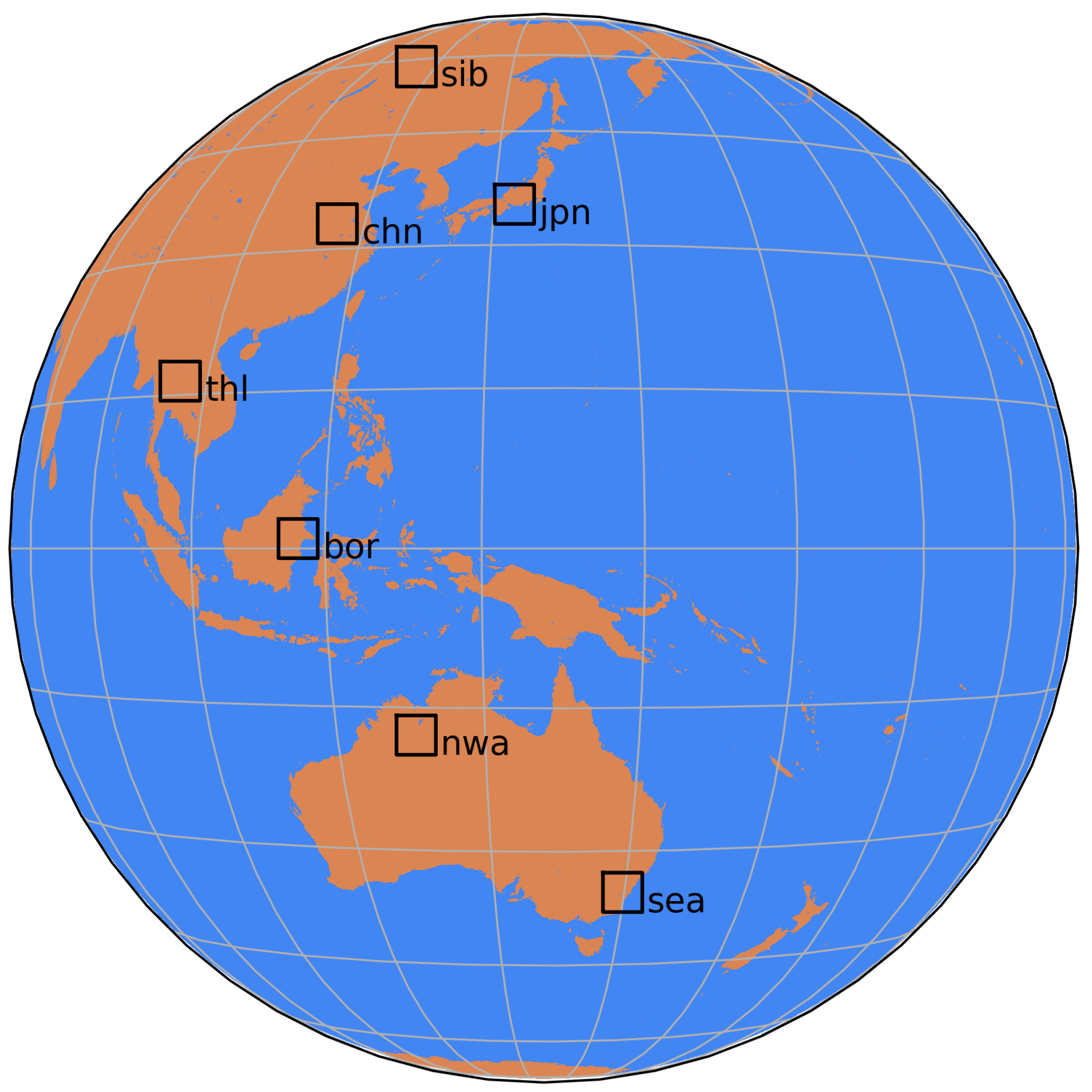
Figure 1. Locations of the case study areas selected for analysis in this paper depicted on the AHI full disk.
Remotesensing 15 03521 g001
Figure 2. Pixel training comparisons for selected pixels in the bor_l group. (Left) shows the spatial distribution of pixels selected during the training process relative to the 50-pixel radius selection area, with the corresponding contextual selection area inside the green box. (Right) depicts the pixel trajectories over the image set examined for training, with the prediction target pixel value shown in red, the STS training pixel values in blue, and the surrounding context pixel values in green. The distribution of values in the prediction image is shown at time t for both prediction methods, with their respective means shown as coloured crosses in comparison to the recorded brightness temperature, which is shown as a red dot. The pixels shown are (a) [2724, 1515], (b) [2724, 1517], and (c) [2724, 1518] and the prediction time t is 2016-067 04:20 UTC.
Remotesensing 15 03521 g002
Figure 3. Flowchart of the STS selection and estimation process for prediction of a single pixel.
Remotesensing 15 03521 g003
Figure 4. A series of brightness temperature images and related estimations for the thl_j region. From left to right, the AHI B07 brightness temperature at the prediction time, the STS prediction image of the area, the contextual estimation of the area, and the respective differences between the AHI image and STS estimates and the AHI image and contextual estimate. The differences highlight positions where the recorded image value was higher than the estimation (red) and vice versa (blue). The prediction times shown here are (a) 2016-082 02:10 UTC, (b) 2016-082 05:20 UTC, (c) 2016-082 08:10 UTC, and (d) 2016-082 17:10 UTC.
Remotesensing 15 03521 g004
Figure 5. Examples of common errors in contextual brightness temperature estimation and the results using STS in similar conditions: (a) the bor_g region at 2016-052 07:50 UTC; (b) the nwa_f region at 2016-315 00:50 UTC; (c) the bor_f region at 2016-068 16:10 UTC; (d) the chn_e region at 2016-241 04:50 UTC.
Remotesensing 15 03521 g005
Table 1. Specifications for the timeframes, area of the AHI disk, and UTC time offsets for each of the case study areas examined.
CS AreaStart DateEnd DateUTC HoursSectors Modelled
sea2016-03-302016-04-2902:00–02:50sea_b: [4450, 4499, 3050, 3099]
05:00–05:50sea_c: [4500, 4549, 3050, 3099]
14:00–14:50sea_e: [4400, 4449, 3100, 3149]
23:00–23:50sea_f: [4450, 4499, 3100, 3149]
sea_h: [4550, 4599, 3200, 3149]
sea_j: [4400, 4449, 3150, 3199]
sea_k: [4450, 4499, 3150, 3199]
nwa2016-10-232016-11-2200:00–00:50nwa_b: [3650, 3699, 2000, 2049]
03:00–03:50nwa_c: [3700, 3749, 2000, 2049]
06:00–06:50nwa_e: [3600, 3649, 2050, 2099]
15:00–15:50nwa_f: [3650, 3699, 2050, 2099]
nwa_g: [3700, 3749, 2050, 2099]
nwa_p: [3650, 3699, 2150, 2199]
nwa_q: [3700, 3749, 2150, 2199]
bor2016-02-142016-03-1501:00–01:50bor_a: [2600, 2649, 1400, 1449]
04:00–04:50bor_f: [2650, 2699, 1450, 1499]
07:00–07:50bor_g: [2700, 2749, 1450, 1499]
16:00–16:50bor_h: [2750, 2799, 1450, 1499]
bor_j: [2600, 2649, 1500, 1549]
bor_l: [2700, 2749, 1500, 1549]
bor_p: [2650, 2699, 1550, 1599]
thl2016-02-282016-03-2902:00–02:50thl_a: [1800, 1849, 800, 849]
05:00–05:50thl_c: [1900, 1949, 800, 849]
08:00–08:50thl_j: [1800, 1849, 900, 949]
17:00–17:50thl_k: [1850, 1899, 900, 949]
thl_m: [1950, 1999, 900, 949]
thl_p: [1850, 1899, 950, 999]
thl_q: [1900, 1949, 950, 999]
chn2016-08-272016-09-2601:00–01:50chn_a: [1000, 1049, 1600, 1649]
04:00–04:50chn_b: [1050, 1099, 1600, 1649]
07:00–07:50chn_e: [1000, 1049, 1650, 1699]
16:00–16:50chn_g: [1100, 1149, 1650, 1699]
chn_k: [1050, 1099, 1700, 1749]
chn_m: [1150, 1199, 1700, 1749]
chn_q: [1100, 1149, 1750, 1799]
jpn2016-05-032016-06-0200:00–00:50jpn_b: [950, 999, 2500, 2549]
03:00–03:50jpn_e: [900, 949, 2550, 2599]
06:00–06:50jpn_f: [950, 999, 2550, 2599]
15:00–15:50jpn_j: [900, 949, 2600, 2649]
jpn_k: [950, 999, 2600, 2649]
jpn_n: [900, 949, 2650, 2699]
jpn_p: [950, 999, 2650, 2699]
sib2016-05-102016-06-0901:00–01:50sib_b: [250, 299, 2000, 2049]
04:00–04:50sib_d: [350, 399, 2000, 2049]
07:00–07:50sib_j: [200, 249, 2100, 2149]
16:00–16:50sib_l: [300, 349, 2100, 2149]
sib_m: [350, 399, 2100, 2149]
sib_n: [200, 249, 2150, 2199]
sib_r: [350, 399, 2150, 2199]
Table 2. Accuracy of estimation techniques against brightness temperature values from the assessed images by case study area; Δ σ is the percentage change between the standard deviations of the contextual and STS estimation methods.
Anomalies RetainedAnomalies Removed
ContextSTS ContextSTS
Site μ (K) σ (K) μ (K) σ (K) Δ σ % μ (K) σ (K) μ (K) σ (K) Δ σ %
sea0.0041.3280.0061.066−19.70.0141.1440.0110.849−25.8
nwa0.0201.3480.0521.292−4.10.0391.1470.0781.025−10.6
bor0.0341.2390.1421.42915.30.0321.0450.1491.20315.1
thl0.0101.2740.0450.849−33.40.0321.1050.0480.665−39.8
chn0.0110.9370.0470.757−19.2−0.0060.8140.0650.635−22.0
jpn0.0241.5760.0271.213−23.0−0.0131.4130.0181.040−26.4
sib0.0081.541−0.0212.13938.80.0171.327−0.0051.77934.0
Table 3. Breakdown of the availability of temperature values (in percentages) using the two estimation methods against total image pixels present; n BT Obs (number of brightness temperature observations) denotes the number of cloud-free image pixels out of the total possible number, denoted as Total Pixel Obs.
SiteTotal Pixel Obsn BT Obs% Context-Image% STS-Image
sea2,142,4721,253,86793.96120.17
nwa2,170,0001,634,66296.65116.40
bor1,694,4601,028,49190.68131.03
thl2,162,5601,715,68197.23112.96
chn2,149,0441,153,59395.10118.34
jpn1,754,724725,49390.68119.36
sib2,168,264801,32990.19117.36
Disclaimer/Publisher’s Note: The statements, opinions and data contained in all publications are solely those of the individual author(s) and contributor(s) and not of MDPI and/or the editor(s). MDPI and/or the editor(s) disclaim responsibility for any injury to people or property resulting from any ideas, methods, instructions or products referred to in the content.