Article

Multi-Level Difference Network for Change Detection from Very High-Resolution Remote Sensing Images: A Case Study in Open-Pit Mines

College of Geoscience and Surveying Engineering, China University of Mining and Technology-Beijing, Beijing 100083, China
*
Author to whom correspondence should be addressed.
Remote Sens. 2023, 15(14), 3482; https://doi.org/10.3390/rs15143482
Submission received: 16 May 2023 / Revised: 7 July 2023 / Accepted: 8 July 2023 / Published: 11 July 2023

Abstract

:
Automatic change detection based on remote sensing is playing an increasingly important role in the national economy construction. To address the problem of limited change detection accuracy in existing single-level difference networks, this study proposes the Multi-level Difference Network (MDNet) for automatic change detection of ground targets from very high-resolution (VHR) remote sensing images. An early-difference network and a late-difference network are combined by MDNet to extract multi-level change features. The early-difference network can focus on change information throughout to reduce the spurious changes in the change detection results, and the late-difference network can provide deep features of a single image for reducing rough boundaries and scattered holes in the change detection results, thus improving the accuracy. However, not all high-level features extracted by MDNet contribute to the recognition of image differences, and the multi-level change features suffer from cross-channel heterogeneity. Stacking them directly on channels does not make effective use of change information, thus limiting the performance of MDNet. Therefore, the Multi-level Change Features Fusion Module (MCFFM) is proposed in this study for the effective fusion of multi-level change features. In the experiments, the publicly available open-pit mine change detection (OMCD) dataset was used first to achieve a change detection of open-pit mines over a large area, with an F1-score of 89.2%, increasing by 1.3% to 5.9% compared to the benchmark methods. Then, a self-made OMCD dataset was used to achieve an F1-score of 92.8% for the localized and fine-scale change detection in open-pit mines, which is an improvement of 0.7% to 5.4% compared to the benchmark methods. Finally, the Season-varying Change Detection Dataset is used to verify that the MDNet proposed can detect changes in other scenarios very well. The experimental results show that the proposed MDNet has significantly improved the performance of change detection on the three datasets compared with six advanced deep learning models, which will contribute to the development of change detection with VHR remote sensing images.

1. Introduction

Change detection aims at identifying significant differences between ground targets or phenomena in multi-temporal remote sensing images and is one of the most important means by which humans can observe surface changes in the earth. It has been applied to several fields, such as urban monitoring [1,2], forest monitoring [3], open-pit mine monitoring [4,5,6], and disaster assessment [7].
With the rapid development of remote sensing technology, the increasing availability of Earth observation data from various satellites, such as WorldView, QuickBird, ZY-3, GaoFen, Sentinel, and Landsat, have made remote-sensing-based change detection a widespread concern among researchers [8]. Among them, detailed information, such as the texture, spectrum, and location of ground targets, can be captured at a finer scale by VHR remote sensing images [9]. Therefore, VHR remote sensing images are considered one of the important data sources for change detection and serve related studies [10,11,12].
Due to the non-negligible disadvantages of visual interpretation for change detection, such as high costs and low efficiency, several traditional and automatic methods have been proposed. Some of the most widely used methods include mainly algebraic-based methods, transformation-based methods, and classification-based methods. (1) Algebraic-based methods: algebraic operations or transformations are performed on multi-temporal remote sensing images to obtain change maps, such as change vector analysis (CVA) [13], image regression [14], and image differencing [15]. The key to this type of method is determining the threshold of change. As there is not yet a reliable method for selecting the change threshold, their accuracy is strongly subject to human influence. (2) Transformation-based methods: change maps are obtained by data down-dimensioning and highlighting difference information on multi-temporal images, such as tasseled cap transformation [16] and principal component analysis (PCA) [17]. However, this type of method is likely to affect the location of change areas and the determination of the change types. (3) Classification-based methods: change maps are obtained by comparing multiple classification maps [18,19,20]. This strategy of using classification followed by change detection is prone to error accumulation. Although the efficiency of these methods has been improved, they share a common and non-negligible disadvantage in that they all conduct comparative analysis on handcrafted features (textures, spectra, etc.) to detect changes, which makes it difficult to accurately represent the various types of complex environments in remote sensing images.
Since the successful application of deep learning to computer vision, many CNNs (Convolutional Neural Networks) have been proposed, such as FCN (Fully Convolutional Networks), PSPNet (Pyramid Scene Parseing Network), DeepLabv3+, and SegNet [21,22]. These CNNs demonstrate a powerful learning capability for structured features of images and provide new research ideas for change detection [23,24]. The existing research on deep-learning-based change detection can be divided into early-difference networks and late-difference networks according to the data fusion methods of multi-temporal remote sensing images. The general flow of change detection for both types of networks is shown in Figure 1. (1) Early-difference networks: two images are fused by channel stacking or taking the absolute difference to meet the single input of this type of network. The change information of two images is always present from input to output, so the networks can focus on the discovery of change regions throughout, without error accumulation. However, the early layers of the networks are unable to provide deep features of a single image for images reconstruction (the deep features here refer to information such as the actual boundaries and internal integrity of the ground targets), resulting in change detection results that are prone to rough boundaries and scattered holes [5,25,26]. (2) Late-difference networks: the late-difference networks are the opposite of the early-difference networks in that they use two inputs to receive two images, with the early layers extracting the deep features of the two images and the late layers obtaining the change information by taking the absolute difference. Although the early layers can provide deep features of a single image to reconstruct the images, the two-stage approach to extracting change features is prone to error accumulation, resulting in change detection results that are prone to spurious changes, such as background changes due to season and shadows [6,27,28]. In summary, while some progress has been made in deep-learning-based change detection research, the problem of the existing single-level difference networks prone to change detection results with rough boundaries, scattered holes, and spurious changes remains to be solved (early-difference networks and late-difference networks are collectively known as single-level difference networks).
To address the above problems, this study constructs an early-difference network and a late-difference network, and then combines them to propose a multi-level difference network (MDNet) for change detection from VHR remote sensing images. MDNet enables reconstructing images and reducing error accumulation to be conducted together in the network, i.e., it is possible to simultaneously optimize the rough boundaries, scattered holes, and spurious changes in the change detection results, and improve the accuracy. Specifically, the architecture of the encoder-decoder is used by MDNet for end-to-end change detection. The encoder consists of a late-difference network and an early-difference network. After the two images are input into the late-difference network, first, the deep features are extracted separately, and then, the change features are extracted. The absolute difference between the two images is input into the early-difference network, and the change features are extracted directly. To effectively fuse the two heterogeneous change features, the Multi-level Change Features Fusion Module (MCFFM) proposed in this study is used in the decoder for the weighted fusion of the two. Further, the shallow information from the encoder is introduced in the decoder using skip connections [29], which is to reduce information loss due to increasing network depth, then reduce missed detections in small areas of changes. For example, landslides are small ground targets in remote sensing images, and the proportion of pixels may even be less than 6% in some datasets [21,30]. Therefore, reducing the missed detection in small areas of changes is crucial to improving the accuracy of similar tasks.
The main contributions of this study include:
(1)
MDNet for high-precision change detection from VHR remote sensing images is proposed by combining an early-difference network and a late-difference network. This study demonstrates that multi-level difference networks are more advantageous than the widely used single-level difference networks for change detection from VHR remote sensing images.
(2)
MCFFM for the effective fusion of multi-level change features is proposed, which further enhances the performance of MDNet.
(3)
The change detection of open-pit mines over a large area is implemented based on the publicly available OMCD dataset, and experimental results on this dataset show that the proposed MDNet has the best change detection performance. Then, an OMCD dataset containing a total of two open-pit mines was produced, and localized and fine-scale change detection of open-pit mines was implemented on this dataset. The experimental results show that the proposed MDNet outperforms all benchmark methods.
(4)
A multi-scenario suitability analysis was carried out using the Season-varying Change Detection Dataset, and the results showed that MDNet could detect changes in other scenarios very well.

2. Methods

2.1. MDNet

The architecture of encoder-decoder is used by MDNet for end-to-end change detection, with the encoder performing the extraction of multi-level change features, and the decoder performing the fusion of multi-level change features and generation of change detection results. Its structure is shown in Figure 2.
The encoder consists of a late-difference network and an early-difference network, both of which use ResNet50 for extracting features, as the residual structure of ResNet50 allows it to better extract the deep features of the images. In the encoder, the late-difference network takes two images as input, then layer-by-layer down-sampling is used to extract multiscale features from each of the two images, and the absolute difference between the features is calculated layer-by-layer to obtain multiscale change features. The early-difference network takes the absolute difference between the two images as input and extracts the multi-scale change features directly. In the decoder, the two change features extracted by the encoder with large differences are first stacked in channels, and then the MCFFM proposed in this study is used to effectively fuse the two, followed by layer-by-layer up-sampling, and finally, the change detection result is output. It is worth noting that the information loss in the late layers of the network increases with the depth of the network. Therefore, multi-scale change information from the early layers is introduced into the decoder by the skip connections and MCFFM to reduce information loss and improve change detection accuracy. Finally, to reduce the effect of sample imbalance on the training process, this study used a joint loss function to calculate the loss of MDNet [31].
For the feature map size after feature extraction, taking the 3 × 512 × 512 images as an example (3 × 512 × 512 means that the image has 3 channels, a height of 512, and a width of 512), it is input to the MDnet and then passes through the encoder and decoder in turn, finally outputting a 2 × 512 × 512 change map. In the encoder, the sizes of the 5 feature maps are 64 × 512 × 512, 128 × 256 × 256, 256 × 128 × 128, 512 × 64 × 64, and 1024 × 32 × 32, in that order. In the decoder, the 4 feature maps have sizes of 512 × 64 × 64, 256 × 128 × 128, 128 × 256 × 256, and 64 × 512 × 512, in that order.

2.2. ResNet50 for Feature Extraction

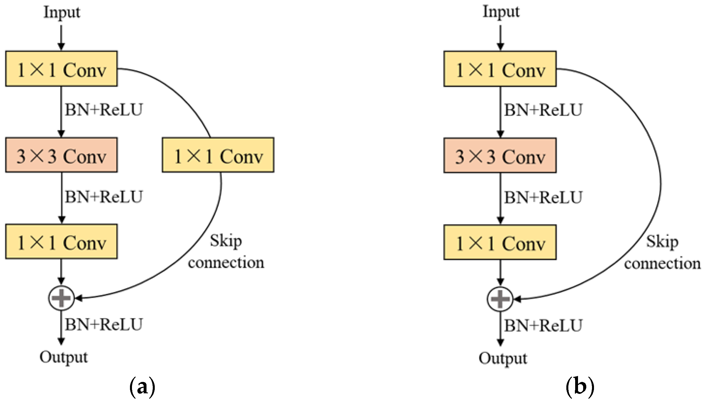
ResNet50 is a residual network proposed by He et al. [32] to mitigate the performance degradation of deep neural networks due to increasing network depth. The residual blocks of ResNet50 consist of two types: convolutional block and identity block, as shown in Figure 3. The backbone of both residual blocks is two 1 × 1 convolutions, one 3 × 3 convolution, and several batch normalizations and ReLUs. The difference between the 2 is that the convolutional block adds a 1 × 1 convolution at the skip connection, whereas the identity block does not. The role of the convolutional block is to change the size of the feature map and save computational resources. The identity block is used to increase the depth of the network and extract deeper features.
ResNet50 can be divided into five stages from input to output, as shown in Figure 4. Firstly, stage 1 changes the feature map size to 1/4 of the original by 7 × 7 convolution and 3 × 3 MaxPool. Stages 2 to 5 proceed in sequence, each consisting of a convolutional block and several identity blocks.

2.3. MCFFM for Multi-Level Change Feature Fusion

Not all of the high-level features extracted by MDNet contribute to the recognition of image differences, and irrelevant features can instead make network training more difficult. In addition, there is a problem of heterogeneity between the two types of change features extracted by the late-difference network and the early-difference network in MDNet. So, direct up-sampling of the two after channel stacking does not make full use of the effective change information. With this in mind, this study proposes the MCFFM for an effective fusion of the two change features, as shown in Figure 5.
To obtain accurate spatial information about the change feature map, MCFFM decomposes the global pooling in the X and Y directions [33], and Figure 6 shows an example of MaxPool. Specifically, the global features of the change feature map (C × H × W, where C, H, W represent the number of channels, height, and width, respectively) were first extracted along the X and Y directions using pooling kernels of size H × 1 and 1 × W, respectively. Then, the MaxPool feature Z m a x c w ( w ) and AvgPool feature Z a v g c w ( w ) of the channel c at width w can be expressed by Equations (1) and (2), respectively. Similarly, the MaxPool feature Z m a x c h ( h ) and AvgPool feature Z a v g c h ( h ) of the channel c at height h can be expressed by Equations (3) and (4), respectively, where x represents the value of the pixel in the image.
Z m a x c w ( w ) = max 0 j < H [ x c ( w , j ) ]
Z a v g c w ( w ) = 1 H 0 j < H x c ( w , j )
Z m a x c h ( h ) = max 0 i < W [ x c ( i , h ) ]
Z a v g c h ( h ) = 1 W 0 i < W x c ( i , h )
After obtaining the global features in both directions, matrix addition is performed on the 2 feature maps in the X direction, then 1 × 1 convolution, batch normalization, ReLU, 1 × 1 convolution, and Sigmoid are performed in turn to finally obtain the weight matrix Xw (C × 1 × W). Similarly, the weight matrix Yw (C × H × 1) in the Y direction is obtained in the same way. Next, the weight map Zw (C × H × W) with information about the exact location is calculated using the formula Zw = Yw × Xw. Finally, the input and Zw are multiplied element by element to obtain the fused change feature.
In summary, MCFFM is essentially an attention-based fusion method that can automatically discover the importance of change features in both spatial and channel dimensions. First, MCFFM computes change features with precise location information using two pooling methods in two directions, resulting in a weight map that accurately represents change pixels and non-change pixels (high weights for change pixels and low weights for non-change pixels). Then, MCFFM compresses and expands the change feature map in the channel dimension through operations, such as 1 × 1 convolution, batch normalization, ReLU, 1 × 1 convolution, and Sigmoid, which effectively constructs the dependencies between channels. As a result, the important channel information is preserved, and the unwanted channel information is discarded, thus solving the problem of cross-channel heterogeneity in multi-level change features fusion.

2.4. Joint Loss Function for Loss Calculation

The loss function is used to calculate the difference between the reference and the predicted value. To reduce the impact of sample imbalance on network training, this study used a joint loss function ( J L ) consisting of a cross-entropy loss function ( C E L ) and a DICE coefficient loss function ( D L ) to train MDNet [31]. The joint loss function can combine pixel-related losses and region-related losses, which is defined in Equation (5).
J L = C E L + D L
The CEL can effectively measure the discrepancy between the true and predicted distributions, which is related to pixels and defined in Equation (6).
C E L = 1 n i = 1 n ( y i l o g y ^ i + ( 1 y i ) log ( 1 y ^ i ) )
where n is the number of pixels, y i and y ^ i represent the reference value and predicted probability value, respectively. y i { 0 , 1 } and y i ^ [ 0 , 1 ] .
D L can effectively calculate the overlap between the reference and predicted values, which is related to the regions and defined in Equation (7).
D L = 1 D I C E = 1 2 | X Y | | X | + | Y |
where D I C E denotes the D I C E coefficient; X and Y denote the two sample sets, respectively; | X Y | denotes the intersection between X and Y ; and | X | and | Y | denote the number of elements in X and Y , respectively. In change detection, X denotes the set of standard change pixels, and Y denotes the set of change pixels predicted by the network.

3. Experiments

3.1. Datasets

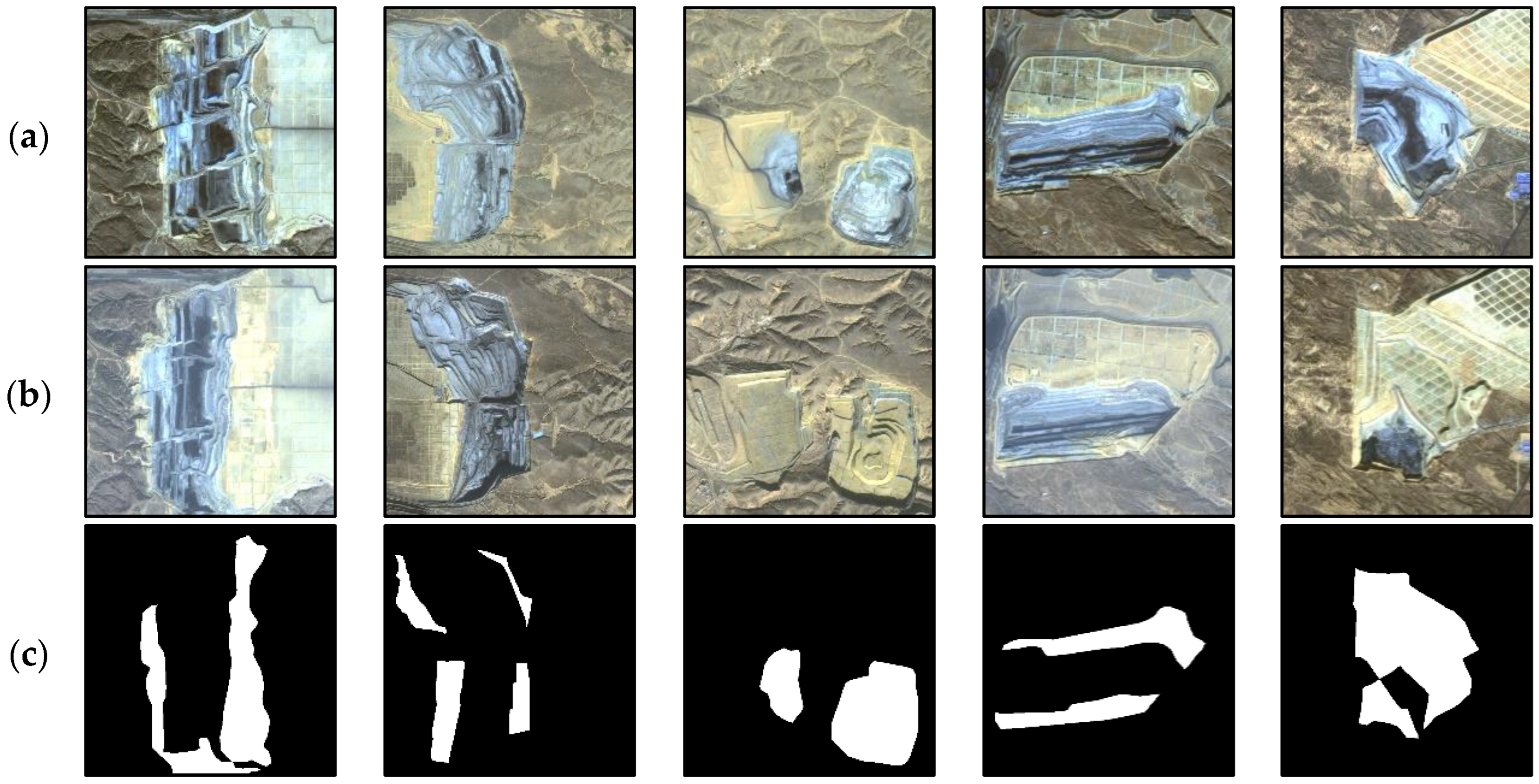
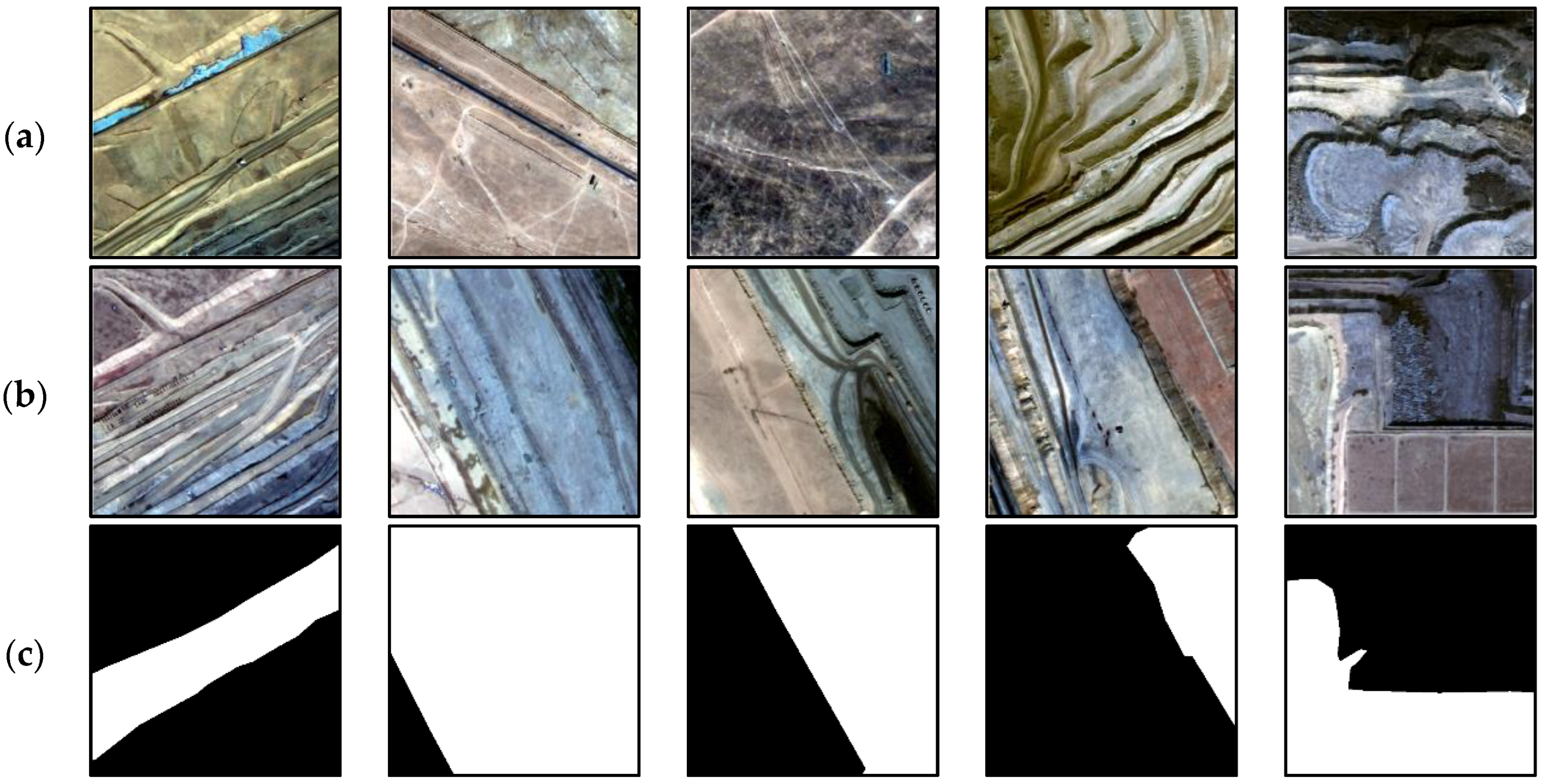
Three datasets were tested and analyzed in the experiments, in order to validate the effectiveness of MDNet applied to VHR remote sensing image change detection. Dataset 1 is an OMCD dataset with 2 m spatial resolution produced by Li et al. [6] and includes a total of 39 open-pit mines. This dataset is used for change detection in open-pit mines over a large area, some of which are shown in Figure 7. Dataset 2 consists of a self-generated OMCD dataset, featuring a spatial resolution of 1 m and encompassing a total of 2 open-pit mines. This dataset is a localized and fine-scale open-pit mines change detection dataset; therefore, it has a higher resolution than Dataset 1, part of which is shown in Figure 8. The use of these two datasets allows for a more comprehensive evaluation of MDNet. Dataset 3 is a publicly available dataset called the Season-varying Change Detection Dataset, which was used to demonstrate that MDNet can handle a wider range of scenarios, some of which are shown in Figure 9.
(1)
Dataset 1: publicly available OMCD dataset (Figure 7, Download link: https://figshare.com/s/ae4e8c808b67543d41e9, accessed on 14 December 2022). The area covered by this dataset falls within a concentration of open-pit mines, located in Erdos, Inner Mongolia Autonomous Region and Yulin, Shaanxi Province, China. The dataset was generated from the GaoFen-6 satellite (Table 1 shows its parameters) images with a spatial resolution of 2 m, including 3 bands of red, green, and blue, and covering the years 2019, 2020, and 2021. The change reference images in this dataset were obtained by visual interpretation, and 31 open-pit mines were used for network training and 8 for network testing. After cropping to 256 × 256 pixels, the training set consisted of 660 image pairs, and the test set consisted of 212 image pairs. Finally, the training set was enhanced (rotated, vertically flipped, and horizontally flipped) to 2640 image pairs.
(2)
Dataset 2: self-made OMCD dataset (Figure 8, Download link: https://figshare.com/s/037aae7bb5fd3c333282, accessed on 28 June 2023). This dataset includes two GaoFen-2 satellite (Table 2 shows its parameters) images of the Shengli No. 1 open-pit mine and Shengli West No. 3 open-pit mine in Xilinhot, Inner Mongolia Autonomous Region, China, on 24 March 2015 and 20 March 2020, with significant changes due to mining activities in both phases of the images. The spatial resolution of the images is 1 m. The images were cropped to 512 × 512 pixels to obtain a total of 52 pairs of images. Then, 42 pairs of images were randomly selected for model training, and the remaining 10 pairs were used for model testing. After data enhancement, the image pairs used for model training reached 168.
(3)
Dataset 3: Season-varying Change Detection Dataset [34] (Figure 9, Download link: https://drive.google.com/file/d/1GX656JqqOyBi_Ef0w65kDGVto-nHrNs9/edit, accessed on 4 June 2018). This dataset contains 7 pairs of 4725 × 2200 pixels and 4 pairs of 1900 × 1000 pixels remote sensing images, which have true seasonal changes. The images were all obtained from Google Earth and covered different areas with a spatial resolution of 3–100 cm. In the production of standard change maps, only the addition and disappearance of ground targets were considered changes. After cropping, the training set included 10,000 pairs of images, and the test set included 3000 pairs of images. This dataset was chosen to demonstrate that MDNet can handle more scenarios because it contains a relatively wide variety of scenarios and ground targets. As shown in Figure 9, the first column of images shows the change in cars and highways, the second column shows the change in roads, and the third column shows the change in buildings.

3.2. Experimental Setup

The experiments were conducted on a desktop computer with an Intel Xeon Gold 5118 central processing unit, 32 G of RAM, and an NVIDIA GeForce RTX2080Ti graphics card. To verify the advanced performance of the proposed MDNet, six advanced deep learning networks were selected for comparison in this study, including two classical semantic segmentation networks, PSPNet [21] and DeepLabv3+ [21], two early-difference change detection networks, CSA-CDGAN [26] and DA-UNet++ [5], and two late-difference change detection networks, SNUNet [27] and SMCDNet [6].
Several parameters in the training process need to be determined to achieve the best performance of the proposed MDNet and the other six networks, including loss function, optimizer, learning rate, batch size, and epochs (maximum number of training iterations). For MDNet, the joint loss function (Cross-entropy loss and DICE coefficient loss) was chosen to calculate the loss during the training process, as it reduces the impact of sample imbalance on network training. The Adam (Adaptive moment estimation) was chosen as a parametric optimizer because of its low memory consumption and robustness, and it is one of the very widely used parametric optimizers in deep learning [35]. The learning rate was determined by parameter tuning with a test range of {0.00005, 0.0001, 0.0005, 0.001, 0.005, 0.01}, and the optimal learning rate was determined to be 0.0001 based on the loss. Studies have pointed out that larger batch size is beneficial to improve network accuracy [36], but limited by computer memory, data volume, and image size, this study set the batch size to seven when training publicly available OMCD dataset, two when training self-made OMCD dataset, and seven when training Season-varying Change Detection Dataset. To ensure that the loss curve of the network training can eventually stabilize, the epoch is set to 200. For the other six networks, the parameters were empirically adjusted by referring to relevant literature, and their optimal parameter combinations were finally determined, as shown in Table 3. Among them, the three values of batch size denote the parameters for the publicly available OMCD dataset, self-made OMCD dataset, and Season-varying Change Detection Dataset, respectively.

3.3. Accuracy Evaluation

In this study, four accuracy evaluation metrics commonly used for change detection were selected to quantitatively evaluate the results, including Precision, Recall, F1-score, and IoU (Intersection over Union), which are defined in Equations (8)–(11). Precision represents the ratio of correctly predicted changed pixels to all predicted changed pixels; Recall represents the ratio of correctly predicted changed pixels to all reference changed pixels; F1-score is used for a comprehensive evaluation of model accuracy; and IoU is a standard performance measure for semantic segmentation.
P r e c i s i o n = T P T P + F P
R e c a l l = T P T P + F N
F 1 s c o r e = 2 × P r e c i s i o n × R e c a l l P r e c i s i o n + R e c a l l
I o U = T P T P + F P + F N
where T P is the number of correctly predicted changed pixels; F P is the number of incorrectly predicted changed pixels; F N is the number of missing changed pixels.

3.4. Experimental Results

3.4.1. Results of Publicly Available OMCD Dataset

Figure 10 shows the detection results of seven networks applied to the publicly available OMCD dataset. It is not difficult to see that the detection results of MDNet are much closer to the ground truth and significantly better than the other six networks. As can be seen from regions 1, 3, and 6, the detection results of MDNet only have fewer false detections, and are well able to ignore pseudo changes due to image backgrounds, etc. From regions 2, 4, and 5, it can be found that the detection results of MDNet have more complete interiors and smoother boundaries, and can show the whole change area of the open-pit mine well, while the detection results of the other networks all have significant omissions and fragmentation.
Table 4 shows the accuracy evaluation of the seven networks on this dataset. The proposed MDNet achieves optimal Recall, F1-score, and IoU with 91.6%, 89.2%, and 80.4%, respectively. There is a significant improvement compared to the other 6 networks, with Recall improving by 3.1% to 6.2%, F1-score by 1.3% to 5.9%, and IoU by 1.9 to 9.0%. SMCDNet achieved an optimal Precision of 87.4%, which is 0.6% higher than MDNet. Among the 6 networks compared, SMCDNet also achieved the best Recall, F1-score, and IoU, with 88.5%, 87.9%, and 78.5%, respectively. In summary, for change detection of ground targets over a large area, the performance and visual effects of MDNet are optimal.

3.4.2. Results of Self-Made OMCD Dataset

Figure 11 shows the detection results of the seven networks on the self-made OMCD dataset. Compared to the other six networks, the detection results of MDNet have fewer false detections in region 1. Compared to the detection results of SMCDNet, DA-UNet++, and DeepLabv3+, the detection results of MDNet showed no significant holes in region 2. Compared to CSA-CDGAN and DeepLabv3+, the detection results of MDNet are complete in region 3. As can be seen from regions 4, 5, and 6, the detection results of MDNet are significantly improved compared to the false and missed detections of the other 6 networks, and the results are much closer to the ground truth.
Table 5 shows the accuracy evaluation of the seven networks on this dataset. The Precision, F1-score, and IoU of MDNet are all optimal, with Precision improving by 0.9% to 6.8%, F1-score by 0.7% to 5.4%, and IoU by 1.3 to 9.0% compared to the other 6 networks. The Recall is optimal for SMCDNet and the second for MDNet, but the former was only 0.3% higher than the latter.
In summary, MDNet achieves the best performance and visual effects not only in the change detection of ground targets over a large area, but also in the localized and fine-scale change detection. Therefore, MDNet can be better applied to the change detection from VHR remote sensing images.

4. Discussion

In order to further analyze the advanced performance of the proposed MDNet, this study presents an in-depth discussion in Section 4.1, Section 4.2, Section 4.3, Section 4.4 and Section 4.5 using the publicly available OMCD dataset as an example. In Section 4.6, this study verifies the multi-scenario suitability of MDNet using the Season-varying Change Detection Dataset. In Section 4.7, some of the future work worth doing is discussed in detail.

4.1. Multi-Level vs. Single-Level

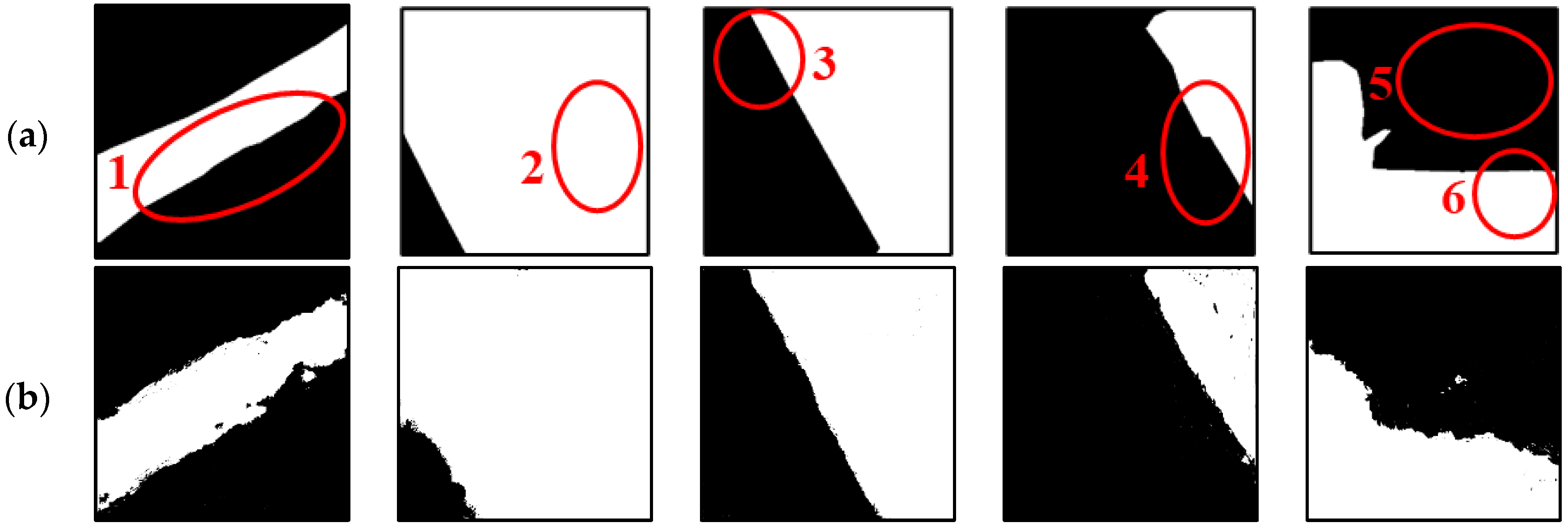
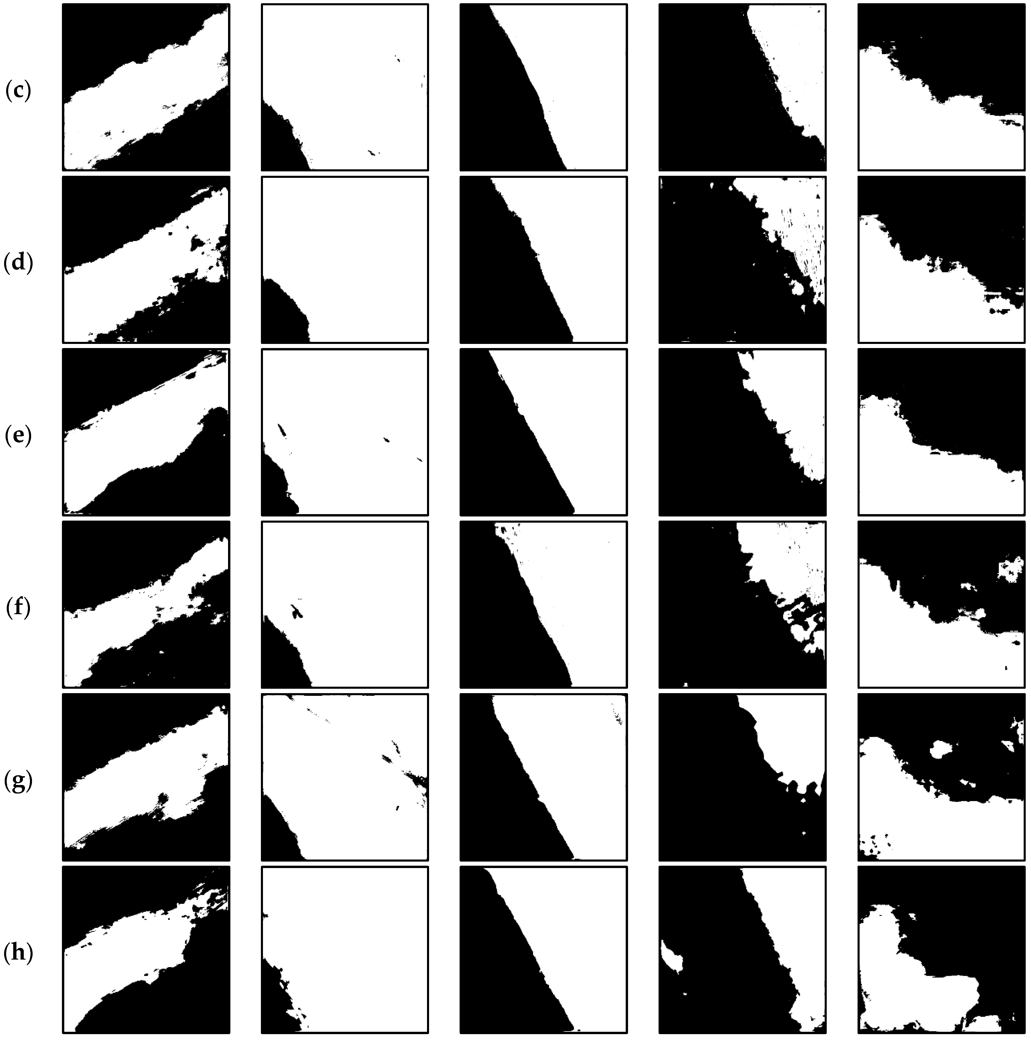
Ablation experiments were designed in this study to demonstrate the effectiveness of MDNet, and Figure 12 shows the change detection results for MDNet and its three ablation networks. As shown in regions 1 and 6, the false detections of the results from MDNet were significantly increased, regardless of whether the early-difference network or the late-difference network was removed. There is also a marked increase in missed areas, such as areas 2, 3, 4, and 5. This is due to the inability of the early-difference network to provide the deep features of a single image for images reconstruction and the error propagation in the late-difference network. It can be seen that multi-level difference networks have an advantage over single-level difference networks in change detection. The completeness of the detection results from MDNet with MCFFM removed is significantly reduced, as the network is unable to effectively fuse the multi-level change features. It is therefore concluded that MCFFM can further improve the performance of multi-level difference networks.
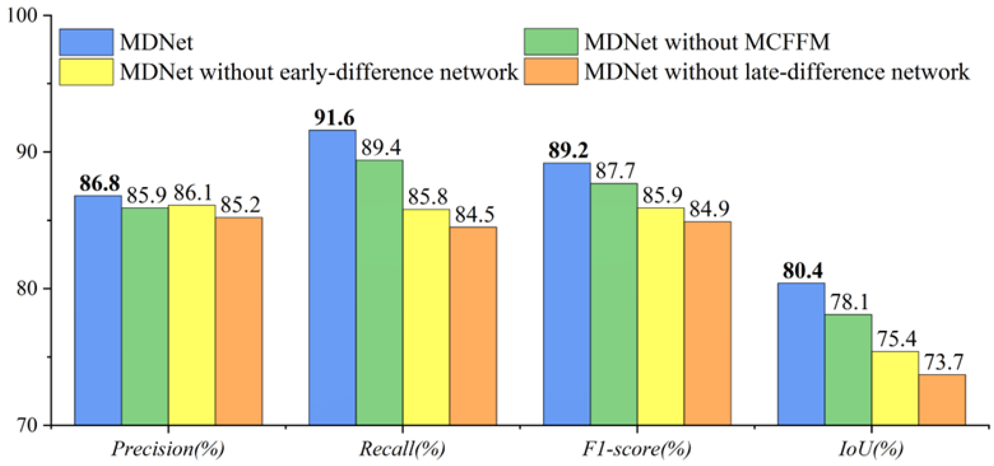
Figure 13 illustrates the accuracy evaluation of MDNet and its three ablation networks. Precision, Recall, F1-score, and IoU for MDNet are 86.8%, 91.6%, 89.2%, and 80.4%, respectively, all of which are optimal. The four evaluation metrics of MDNet after removing one of MCFFM, early-difference network, and late-difference network have all decreased in varying degrees. The ranking of the comprehensive performance for the three ablation networks is MDNet without MCFFM > MDNet without early-difference network > MDNet without late-difference network.
Finally, to ensure that the number of layers in the proposed MDNet is optimal, we tested four cases of increasing or decreasing the number of layers in the network: (1) Case 1: decreasing one layer; (2) Case 2: decreasing two layers; (3) Case 3: increasing one layer; (4) Case 4: increasing two layers. It was then tested with the publicly available OMCD dataset as an example. Table 6 shows the change detection accuracy of MDNet for the four cases. From Table 6, we can see that the MDNet proposed in this paper is optimal and that increasing or decreasing the number of layers will reduce the change detection accuracy of the network. Therefore, it can be concluded that the number of layers in the proposed MDNet is indeed reasonable and optimal.

4.2. Effectiveness Analysis of MCFFM

Currently, the field of computer vision frequently employs attention for feature fusion, so in this study, four commonly used attention modules were selected to compare with the proposed MCFFM, namely, CA (Coordinate Attention) [33], CBAM (Convolutional Block Attention Module) [37], BAM (Bottleneck Attention Module) [38], and SENet (Squeeze-and-Excitation Networks) [39]. Figure 14 illustrates the accuracy evaluation of MCFFM and attention modules as applied to multi-level change feature fusion. It can be found that MCFFM achieves optimal Precision, Recall, F1-score, and IoU, proving that it is better able to fuse multi-level change features. In terms of overall performance, the ranking of the four attention modules is CA > CBAM > BAM > SENet.

4.3. Effectiveness Analysis of Feature Extraction Network

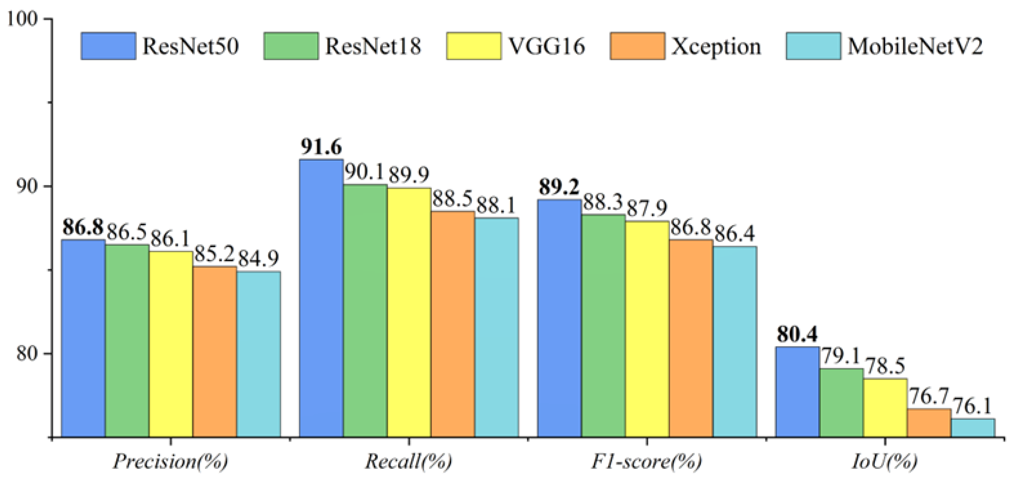
To verify that ResNet50 in MDNet can perform feature extraction better, four commonly used feature extraction networks were selected for comparison in this study, which are ResNet18 [40], VGG16 [41], Xception [6], and MobileNetV2 [42]. Figure 15 shows the accuracy evaluation of MDNet after adding each feature extraction network. It can be found that the change detection performance of MDNet is significantly improved by using ResNet50 for feature extraction compared to the other four feature extraction networks. Ranking of the overall performance for the four feature extraction networks is ResNet18 > VGG16 > Xception > MobileNetV2.

4.4. Comparison of Network Size and Efficiency

To verify the feasibility of the proposed MDNet, statistics on the number of parameters (Figure 16a), network size (Figure 16b), and time cost of network training and testing (Figure 16c) for the seven networks were conducted in this study. Among all networks, MDNet is the largest in number of parameters (7.25 × 10⁷) and network size (277.01 MB). Its time cost of training (65 s/epoch), apart from being significantly higher than DeepLabv3+ (41 s/epoch) and PSPNet (36 s/epoch), is roughly on par with other networks, with a maximum time difference of no more than 7 s/epoch. Its time cost of testing (12 s/epoch) was about the same as all the networks compared, with a maximum time difference of no more than 3 s/epoch. Overall, given the better change detection performance of MDNet and the small difference in time cost between the different networks, its larger number of parameters and network size are acceptable.

4.5. The Training Process of MDNet

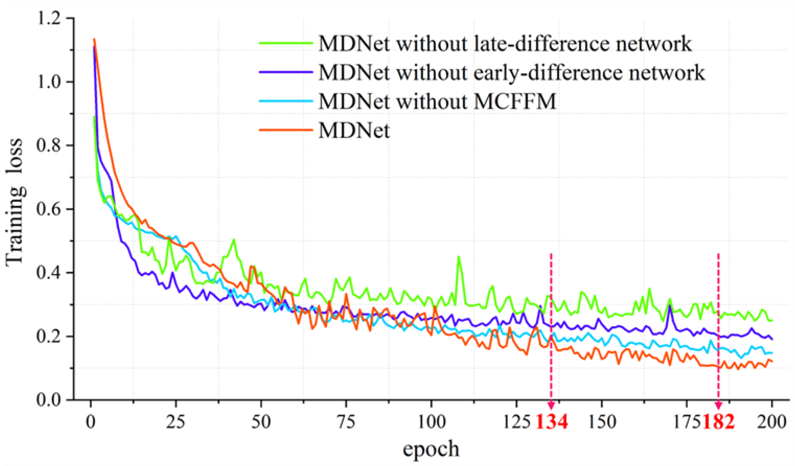
The trend of loss in training can reflect the performance and stability of the network. The training process of MDNet and its three ablation networks is shown in Figure 17. As the number of epoch increases, the loss of the four networks gradually decreases with less fluctuation. After 134 epochs, the loss of MDNet was steadily lower than that of the 3 ablation networks. After 182 epochs, the loss of all 4 networks stabilized. As a result, the proposed MDNet can be trained stably and with lower overall loss, which is more advantageous than single-level difference networks.

4.6. Multi-Scenario Suitability Analysis of MDNet

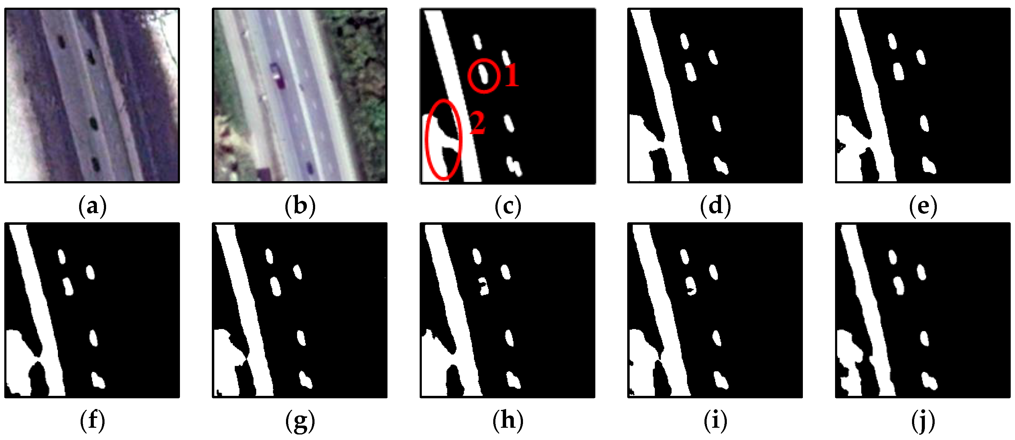
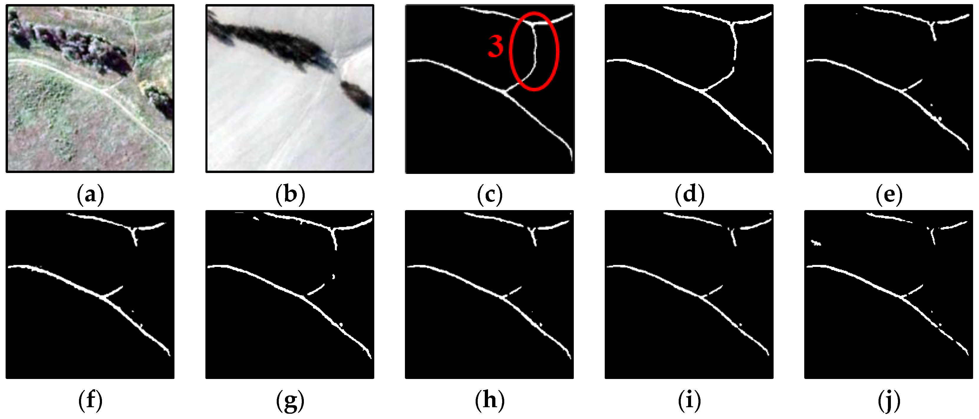
To verify that the MDNet proposed in this study can detect changes in other scenarios very well, a multi-scenario suitability analysis was conducted using the Season-varying Change Detection Dataset. Figure 18 shows the changes in cars and highways. From region 1, it can be seen that the results of MDNet show the changes in cars quite complete, while the results of CSA-CDGAN and DeepLabv3+ are unable to detect the complete cars. From region 2, it can be seen that the results of other networks have more missed areas than the results of MDNet. Figure 19 shows the changes in roads. As can be seen from region 3, all the roads detected by the networks used for comparison have a large number of disconnections and a small number of false detections, while the roads detected by MDNet have only a very small number of disconnections and almost no false detections, which is closest to the ground truth. Figure 20 shows the changes in buildings. From region 4, it can be seen that the change in buildings detected by MDNet is closest to ground truth, with the other networks showing more false detections in their results.
Table 7 shows the accuracy of each network applied to the Season-varying Change Detection Dataset. Except for Recall, the Precision, F1-score, and IoU of MDNet are all optimal and significantly improved compared to other networks.
In summary, for the Season-varying Change Detection Dataset, the visual effect and accuracy of the change detection results for MDNet are significantly better than those of other networks, which indicates that MDNet can detect changes in more scenarios well and has some prospects for generalization.

4.7. Prospects

The multi-level difference network is an idea for constructing change detection networks, which aims at introducing multiple effective and complementary change features to improve the accuracy of change detection. Notably, it is not limited to a specific network structure and has some potential for development. The proposed method is not optimal in terms of network size and training time cost, but it is not significantly different from the other methods. It is worth noting that the proposed method does perform optimally, which is due to the new network architecture and the feature fusion module proposed in this study. In order to work towards a more comprehensive and superior model, the following solutions can be considered for future work: (1) Using pruning algorithms to compress the network and reducing the training time of the network, such as filter-wise, channel-wise, shape-wise, and block-wise pruning. (2) In this study, ResNet50 was chosen for feature extraction because it gives MDNet the best change detection performance among the five tested feature extraction networks. However, its network size is comparatively large (111.67 MB). Therefore, without degrading the accuracy, a smaller feature extraction network can be attempted, such as replacing a moderate amount of conventional convolution in ResNet50 with Group Convolution or Depthwise Separable Convolution to reduce the number of network parameters.
Last but not least, the results of automatic change detection methods inevitably have varying degrees of holes, false change areas, and rough boundaries, which hardly correspond to the actual change of the ground target. For holes and false change areas, optimization can be attempted using the closed and open operations of mathematical morphological operations. For rough boundaries, optimization can be performed using filtering, such as median filtering. All of these operations can be implemented using OpenCV (Open Source Computer Vision Library), but how to determine the parameters for these operations requires more in-depth study.

5. Conclusions

An automatic and accurate change detection method based on VHR remote sensing images is of great importance to the national economy. In this study, to address the problem of limited change detection accuracy in existing single-level difference networks, a novel deep learning model, MDNet, and a multi-level change feature fusion module, MCFFM, are proposed for change detection from VHR remote sensing images. Three datasets were used in the experiments, including the publicly available OMCD dataset, self-made OMCD dataset, and Season-varying Change Detection Dataset. The superiority of MDNet was demonstrated by comparing it with advanced deep learning models, such as SMCDNet, SNUNet, DA-UNet++, CSA-CDGAN, DeepLabv3+, and PSPNet. The following conclusions were drawn from this study:
(1)
The multi-level difference networks are more beneficial than single-level difference networks in achieving high-precision change detection from VHR remote sensing images.
(2)
MCFFM can further enhance the change detection performance of multi-level difference networks, as it can fuse multi-level change features more effectively.
(3)
ResNet50 is a good deep feature extractor for high-resolution remote sensing images.
(4)
Although MDNet has more parameters than all the compared networks, its training and testing time is in the same order of magnitude as all the compared networks, so it is feasible to apply MDNet to change detection for high-resolution remote sensing images.
(5)
MDNet has advanced performance not only in open-pit mines change detection, but also in other scenarios.

Author Contributions

Conceptualization, W.L. and J.L.; Formal analysis, W.L. and J.L.; Funding acquisition, J.L.; Investigation, C.Z. and J.X.; Methodology, W.L., J.L., S.D. and J.X.; Project administration, J.L. and C.Z.; Validation, W.L. and J.X.; Visualization, W.L. and J.X.; Writing—original draft, W.L. and J.L.; Writing—review and editing, J.L. and S.D. All authors have read and agreed to the published version of the manuscript.

Funding

This research was funded by the National Natural Science Foundation of China (Grant number 42271480), the National Key Research and Development Program of China (Grant number 2022YFF1303301), the Open Foundation of the Key Laboratory of Coupling Process and Effect of Natural Resources Elements (Grant number 2022KFKTC001) and the Fundamental Research Funds for the Central Universities (Grant number 2023ZKPYDC10; 2022JCCXDC04).

Data Availability Statement

(1) The publicly available OMCD dataset can be downloaded from this link: https://figshare.com/s/ae4e8c808b67543d41e9, accessed on 14 December 2022. (2) The self-made OMCD dataset can be downloaded from this link: https://figshare.com/s/037aae7bb5fd3c333282, accessed on 28 June 2023. (3) The Season-varying Change Detection Dataset can be downloaded from this link: https://drive.google.com/file/d/1GX656JqqOyBi_Ef0w65kDGVto-nHrNs9/edit, accessed on 4 June 2018.

Conflicts of Interest

The authors declare no conflict of interest.

References

  1. Daudt, R.C.; Le Saux, B.; Boulch, A.; Gousseau, Y. Urban change detection for multispectral earth observation using convolutional neural networks. In Proceedings of the IEEE International Geoscience and Remote Sensing Symposium (IGARSS), Valencia, Spain, 22–27 July 2018. [Google Scholar]
  2. Chen, H.; Shi, Z. A Spatial-Temporal Attention-Based Method and a New Dataset for Remote Sensing Image Change Detection. Remote Sens. 2020, 12, 1662. [Google Scholar] [CrossRef]
  3. Bullock, E.L.; Healey, S.P.; Yang, Z.; Houborg, R.; Gorelick, N.; Tang, X.; Andrianirina, C. Timeliness in forest change monitoring: A new assessment framework demonstrated using Sentinel-1 and a continuous change detection algorithm. Remote Sens. Environ. 2022, 276, 113043. [Google Scholar] [CrossRef]
  4. Xu, Y.L.; Guo, L.; Li, J.; Zhang, C.Y.; Ran, W.Y.; Hu, J.Y.; Mao, H.T. Automatically identifying the vegetation destruction and restoration of various open-pit mines utilizing remotely sensed images: Auto-VDR. J. Clean. Prod. 2023, 414, 137490. [Google Scholar] [CrossRef]
  5. Du, S.; Li, W.; Li, J.; Du, S.; Zhang, C.; Sun, Y. Open-pit mine change detection from high resolution remote sensing images using DA-UNet plus plus and object-based approach. Int. J. Min. Reclam. Environ. 2022, 36, 512–535. [Google Scholar] [CrossRef]
  6. Li, J.; Xing, J.; Du, S.; Du, S.; Zhang, C.; Li, W. Change Detection of Open-pit Mine Based on Siamese Multi-scale Network. IEEE Geosci. Remote Sens. Lett. 2022, 20, 1–5. [Google Scholar]
  7. Bovolo, F.; Bruzzone, L. A split-based approach to unsupervised change detection in large-size multitemporal images: Application to tsunami-damage assessment. IEEE Trans. Geosci. Remote Sens. 2007, 45, 1658–1670. [Google Scholar] [CrossRef]
  8. Peng, D.; Zhang, Y.; Guan, H. End-to-End Change Detection for High Resolution Satellite Images Using Improved UNet plus plus. Remote Sens. 2019, 11, 1382. [Google Scholar] [CrossRef] [Green Version]
  9. Du, S.; Du, S.; Liu, B.; Zhang, X. Incorporating DeepLabv3+ and object-based image analysis for semantic segmentation of very high resolution remote sensing images. Int. J. Digit. Earth 2021, 14, 357–378. [Google Scholar] [CrossRef]
  10. Wu, C.; Zhang, L.; Zhang, L. A scene change detection framework for multi-temporal very high resolution remote sensing images. Signal Process. 2016, 124, 184–197. [Google Scholar] [CrossRef]
  11. Wang, Q.; Zhang, X.; Chen, G.; Dai, F.; Gong, Y.; Zhu, K. Change detection based on Faster R-CNN for high-resolution remote sensing images. Remote Sens. Lett. 2018, 9, 923–932. [Google Scholar] [CrossRef]
  12. Chen, J.; Yuan, Z.; Peng, J.; Chen, L.; Huang, H.; Zhu, J.; Liu, Y.; Li, H. DASNet: Dual Attentive Fully Convolutional Siamese Networks for Change Detection in High-Resolution Satellite Images. IEEE J. Sel. Top. Appl. Earth Obs. Remote Sens. 2021, 14, 1194–1206. [Google Scholar] [CrossRef]
  13. Saha, S.; Bovolo, F.; Bruzzone, L. Unsupervised Deep Change Vector Analysis for Multiple-Change Detection in VHR Images. IEEE Trans. Geosci. Remote Sens. 2019, 57, 3677–3693. [Google Scholar] [CrossRef]
  14. Zhao, R.; Peng, G.H.; Yan, W.d.; Pan, L.L.; Wang, L.Y. Change detection in SAR images based on superpixel segmentation and image regression. Earth Sci. Inform. 2021, 14, 69–79. [Google Scholar] [CrossRef]
  15. Bindschadler, R.A.; Scambos, T.A.; Choi, H.; Haran, T.M. Ice sheet change detection by satellite image differencing. Remote Sens. Environ. 2010, 114, 1353–1362. [Google Scholar] [CrossRef]
  16. Zanchetta, A.; Bitelli, G.; Karnieli, A. Monitoring desertification by remote sensing using the Tasselled Cap transform for long-term change detection. Nat. Hazards 2016, 83, 223–237. [Google Scholar] [CrossRef]
  17. Achour, S.; Elmezouar, M.C.; Taleb, N.; Kpalma, K.; Ronsin, J. A PCA-PD fusion method for change detection in remote sensing multi temporal images. Geocarto Int. 2022, 37, 196–213. [Google Scholar] [CrossRef]
  18. Demirel, N.; Emil, M.K.; Duzgun, H.S. Surface coal mine area monitoring using multi-temporal high-resolution satellite imagery. Int. J. Coal Geol. 2011, 86, 3–11. [Google Scholar] [CrossRef]
  19. Ye, Q.; He, L.; Ying, M.; Lin, Y. Researches on the land-use change detection of mine area based on TM/ETM images. In Proceedings of the 3rd ISPRS International Workshop on Image and Data Fusion (IWIDF), Antu, China, 20–22 August 2013; pp. 91–101. [Google Scholar]
  20. Nascimento, F.S.; Gastauer, M.; Souza-Filho, P.W.M.; Nascimento, W.R.; Santos, D.C.; Costa, M.F. Land Cover Changes in Open-Cast Mining Complexes Based on High-Resolution Remote Sensing Data. Remote Sens. 2020, 12, 611. [Google Scholar] [CrossRef] [Green Version]
  21. Ghorbanzadeh, O.; Xu, Y.; Ghamisi, P.; Kopp, M.; Kreil, D. Landslide4Sense: Reference Benchmark Data and Deep Learning Models for Landslide Detection. IEEE Trans. Geosci. Remote Sens. 2022, 60, 1–17. [Google Scholar] [CrossRef]
  22. Son, S.; Lee, S.H.; Bae, J.; Ryu, M.; Lee, D.; Park, S.R.; Seo, D.; Kim, J. Land-Cover-Change Detection with Aerial Orthoimagery Using SegNet-Based Semantic Segmentation in Namyangju City, South Korea. Sustainability 2022, 14, 12321. [Google Scholar] [CrossRef]
  23. Gao, L.; Hong, D.; Yao, J.; Zhang, B.; Gamba, P.; Chanussot, J. Spectral Superresolution of Multispectral Imagery with Joint Sparse and Low-Rank Learning. IEEE Trans. Geosci. Remote Sens. 2021, 59, 2269–2280. [Google Scholar] [CrossRef]
  24. Wang, X.; Du, J.; Tan, K.; Ding, J.; Liu, Z.; Pan, C.; Han, B. A high-resolution feature difference attention network for the application of building change detection. Int. J. Appl. Earth Obs. 2022, 112, 102950. [Google Scholar] [CrossRef]
  25. Pan, F.; Wu, Z.; Liu, Q.; Xu, Y.; Wei, Z. DCFF-Net: A Densely Connected Feature Fusion Network for Change Detection in High-Resolution Remote Sensing Images. IEEE J. Sel. Topics Appl. Earth Observ. Remote Sens. 2021, 14, 11974–11985. [Google Scholar] [CrossRef]
  26. Wang, Z.; Zhang, Y.; Luo, L.; Wang, N. CSA-CDGAN: Channel self-attention-based generative adversarial network for change detection of remote sensing images. Neural Comput. Appl. 2022, 34, 21999–22013. [Google Scholar] [CrossRef]
  27. Fang, S.; Li, K.; Shao, J.; Li, Z. SNUNet-CD: A Densely Connected Siamese Network for Change Detection of VHR Images. IEEE Geosci. Remote Sens. 2022, 19, 1–5. [Google Scholar] [CrossRef]
  28. Jiang, H.; Hu, X.; Li, K.; Zhang, J.; Gong, J.; Zhang, M. PGA-SiamNet: Pyramid Feature-Based Attention-Guided Siamese Network for Remote Sensing Orthoimagery Building Change Detection. Remote Sens. 2020, 12, 484. [Google Scholar] [CrossRef] [Green Version]
  29. Peng, D.; Bruzzone, L.; Zhang, Y.; Guan, H.; Ding, H.; Huang, X. SemiCDNet: A Semisupervised Convolutional Neural Network for Change Detection in High Resolution Remote-Sensing Images. IEEE Trans. Geosci. Remote Sens. 2021, 59, 5891–5906. [Google Scholar] [CrossRef]
  30. Ghorbanzadeh, O.; Xu, Y.; Zhao, H.; Wang, J.; Zhong, Y.; Zhao, D.; Zang, Q.; Wang, S.; Zhang, F.; Shi, Y.; et al. The Outcome of the 2022 Landslide4Sense Competition: Advanced Landslide Detection from Multisource Satellite Imagery. IEEE J. Sel. Top. Appl. Earth Observ. Remote Sens. 2022, 15, 9927–9942. [Google Scholar] [CrossRef]
  31. Liu, R.; Jiang, D.; Zhang, L.; Zhang, Z. Deep Depthwise Separable Convolutional Network for Change Detection in Optical Aerial Images. IEEE J. Sel. Top. Appl. Earth Obs. Remote Sens. 2020, 13, 1109–1118. [Google Scholar] [CrossRef]
  32. He, K.; Zhang, X.; Ren, S.; Sun, J. Deep Residual Learning for Image Recognition. In Proceedings of the IEEE Conference on Computer Vision and Pattern Recognition (CVPR), Seattle, WA, USA, 27–30 June 2016; pp. 770–778. [Google Scholar]
  33. Xiang, X.; Tian, D.; Lv, N.; Yan, Q. FCDNet: A Change Detection Network Based on Full-Scale Skip Connections and Coordinate Attention. IEEE Geosci. Remote Sens. Lett. 2022, 19, 1–5. [Google Scholar] [CrossRef]
  34. Lebedev, M.A.; Vizilter, Y.V.; Vygolov, O.V.; Knyaz, V.A.; Rubis, A.Y. Change detection in remote sensing images using con-ditional adversarial networks. Int. Arch. Photogramm. Remote Sens. Spat. Inf. Sci. 2018, 42, 565–571. [Google Scholar] [CrossRef] [Green Version]
  35. Kingma, D.P.; Ba, J. Adam: A method for stochastic optimization. arXiv 2014, arXiv:1412.6980. [Google Scholar]
  36. Radiuk, P.M. Impact of training set batch size on the performance of convolutional neural networks for diverse datasets. Inf. Technol. Manag. Sci. 2017, 20, 20–24. [Google Scholar] [CrossRef]
  37. Yin, M.; Chen, Z.; Zhang, C. A CNN-Transformer Network Combining CBAM for Change Detection in High-Resolution Remote Sensing Images. Remote Sens. 2023, 15, 2406. [Google Scholar] [CrossRef]
  38. Park, J.; Woo, S.; Lee, J.Y.; Kweon, I.S. BAM: Bottleneck Attention Module. arXiv 2018, arXiv:1807.06514. [Google Scholar]
  39. Pang, S.; Li, X.; Chen, J.; Zuo, Z.; Hu, X. Prior Semantic Information Guided Change Detection Method for Bi-temporal High-Resolution Remote Sensing Images. Remote Sens. 2023, 15, 1655. [Google Scholar] [CrossRef]
  40. Feng, Y.; Jiang, J.; Xu, H.; Zheng, J. Change Detection on Remote Sensing Images Using Dual-Branch Multilevel Intertemporal Network. IEEE Trans. Geosci. Remote Sens. 2023, 61, 1–15. [Google Scholar] [CrossRef]
  41. Patra, R.K.; Patil, S.N.; Falkowski-Gilski, P.; Lubniewski, Z.; Poongodan, R. Feature Weighted Attention-Bidirectional Long Short Term Memory Model for Change Detection in Remote Sensing Images. Remote Sens. 2022, 14, 5402. [Google Scholar] [CrossRef]
  42. Li, Z.; Tang, C.; Liu, X.; Zhang, W.; Dou, J.; Wang, L.; Zomaya, A.Y.Y. Lightweight Remote Sensing Change Detection with Progressive Feature Aggregation and Supervised Attention. IEEE Trans. Geosci. Remote Sens. 2023, 61, 1–12. [Google Scholar] [CrossRef]
Figure 1. (a) Early-difference strategy; (b) Late-difference strategy.
Remotesensing 15 03482 g001
Figure 2. The structure of MDNet.
Remotesensing 15 03482 g002
Figure 3. (a) Convolutional block; (b) Identity block.
Remotesensing 15 03482 g003
Figure 4. The structure of ResNet50.
Remotesensing 15 03482 g004
Figure 5. The structure of the MCFFM.
Remotesensing 15 03482 g005
Figure 6. Example of MaxPool in the X and Y directions.
Remotesensing 15 03482 g006
Figure 7. Publicly available OMCD dataset (2 m). (a) Pre-temporal image; (b) Post-temporal image; (c) Ground truth.
Remotesensing 15 03482 g007
Figure 8. Self-made OMCD dataset (1 m). (a) Pre-temporal image; (b) Post-temporal image; (c) Ground truth.
Remotesensing 15 03482 g008
Figure 9. Season-varying Change Detection Dataset (3–100 cm). (a) Pre-temporal image; (b) Post-temporal image; (c) Ground truth.
Remotesensing 15 03482 g009
Figure 10. Results of publicly available OMCD dataset. (a) Ground truth; (b) MDNet; (c) SMCDNet; (d) SNUNet; (e) DA-UNet++; (f) CSA-CDGAN; (g) DeepLabv3+; (h) PSPNet.
Remotesensing 15 03482 g010aRemotesensing 15 03482 g010b
Figure 11. Results of self-made OMCD dataset. (a) Ground truth; (b) MDNet; (c) SMCDNet; (d) SNUNet; (e) DA-UNet++; (f) CSA-CDGAN; (g) DeepLabv3+; (h) PSPNet.
Remotesensing 15 03482 g011aRemotesensing 15 03482 g011b
Figure 12. Results of MDNet and three ablation networks. (a) Ground truth; (b) MDNet; (c) MDNet without MCFFM; (d) MDNet without early-difference network; (e) MDNet without late-difference network.
Remotesensing 15 03482 g012aRemotesensing 15 03482 g012b
Figure 13. Accuracy of MDNet and its three ablation networks (where the bold indicates that this network is optimal for this accuracy metric).
Remotesensing 15 03482 g013
Figure 14. Accuracy of different modules for multi-level change features fusion (where the bold indicates that this network is optimal for this accuracy metric).
Remotesensing 15 03482 g014
Figure 15. Accuracy of different feature extraction network (where the bold indicates that this network is optimal for this accuracy metric).
Remotesensing 15 03482 g015
Figure 16. (a) The number of network parameters; (b) Network size; (c) Time cost of network training and testing.
Remotesensing 15 03482 g016aRemotesensing 15 03482 g016b
Figure 17. The training process of MDNet and three ablation networks.
Remotesensing 15 03482 g017
Figure 18. Results of changes in cars and highways. (a) Pre-temporal image; (b) Post-temporal image; (c) Ground truth; (d) MDNet; (e) SMCDNet; (f) SNUNet; (g) DA-UNet++; (h) CSA-CDGAN; (i) DeepLabv3+; (j) PSPNet.
Remotesensing 15 03482 g018
Figure 19. Results of changes in roads. (a) Pre-temporal image; (b) Post-temporal image; (c) Ground truth; (d) MDNet; (e) SMCDNet; (f) SNUNet; (g) DA-UNet++; (h) CSA-CDGAN; (i) DeepLabv3+; (j) PSPNet.
Remotesensing 15 03482 g019
Figure 20. Results of changes in buildings. (a) Pre-temporal image; (b) Post-temporal image; (c) Ground truth; (d) MDNet; (e) SMCDNet; (f) SNUNet; (g) DA-UNet++; (h) CSA-CDGAN; (i) DeepLabv3+; (j) PSPNet.
Remotesensing 15 03482 g020aRemotesensing 15 03482 g020b
Table 1. Parameters of the GaoFen-6 satellite.
BandSpectral Range/μmSpatial Resolution/mWidth/km
Panchromatic Band0.45~0.90290
Multispectral bandsBlue0.45~0.52890
Green0.52~0.60890
Red0.63~0.69890
NIR0.76~0.90890
Table 2. Parameters of the GaoFen-2 satellite.
BandSpectral Range/μmSpatial Resolution/mWidth/km
Panchromatic Band0.45~0.90145
Multispectral bandsBlue0.45~0.52445
Green0.52~0.59445
Red0.63~0.69445
NIR0.77~0.89445
Table 3. Details of parameter settings for each network.
Loss FunctionOptimizerLearning RateBatch SizeEpochs
MDNetJoint loss (Cross-entropy loss and DICE coefficient loss)Adam (Adaptive moment estimation)0.00017, 2, 7200
SMCDNetJoint lossAdam0.00016, 2, 5200
SNUNetJoint lossAdam0.00017, 2, 6200
DA-UNet++Joint lossAdam0.00025, 2, 7200
CSA-CDGANCross Entropy lossRMSprop (Root mean square prop)0.0016, 2, 7200
DeepLabv3+Cross Entropy lossAdam0.0077, 2, 5200
PSPNetJoint lossSGD (Stochastic gradient descent)0.00016, 2, 7200
Table 4. Accuracy of publicly available OMCD dataset.
Type of NetworkPrecision (%)Recall (%)F1-Score (%)IoU (%)
MDNetmulti-level difference86.891.689.280.4
SMCDNetlate-difference87.488.587.978.5
SNUNetlate-difference86.385.786.075.5
DA-UNet++early-difference86.085.885.975.3
CSA-CDGANearly-difference85.885.485.674.8
DeepLabv3+early-difference80.487.483.872.1
PSPNetearly-difference80.686.283.371.4
Table 5. Accuracy of publicly available OMCD dataset (The bolded numbers are accuracy of each network).
Type of NetworkPrecision (%)Recall (%)F1-Score (%)IoU (%)
MDNetmulti-level difference96.089.892.886.6
SMCDNetlate-difference94.290.192.185.3
SNUNetlate-difference93.686.890.181.9
DA-UNet++early-difference95.188.891.884.9
CSA-CDGANearly-difference92.387.689.981.6
DeepLabv3+early-difference91.786.989.280.6
PSPNetearly-difference89.285.787.477.6
Table 6. The impact of increasing or decreasing the number of layers in the MDNet on the accuracy of change detection (the bolded numbers).
Precision (%) Recall (%) F1-Score (%)IoU (%)
MDNet86.891.689.280.4
Case 185.391.188.178.7
Case 284.289.286.676.4
Case 384.890.587.677.9
Case 485.187.686.376.0
Table 7. Accuracy of Season-varying Change Detection Dataset (The bolded numbers are accuracy of each network).
Type of NetworkPrecision (%)Recall (%)F1-Score (%)IoU (%)
MDNetmulti-level difference96.595.796.192.5
SMCDNetlate-difference94.696.095.391.0
SNUNetlate-difference94.895.194.990.4
DA-UNet++early-difference95.895.095.491.2
CSA-CDGANearly-difference94.194.994.589.6
DeepLabv3+early-difference92.994.393.688.0
PSPNetearly-difference95.390.592.886.6
Disclaimer/Publisher’s Note: The statements, opinions and data contained in all publications are solely those of the individual author(s) and contributor(s) and not of MDPI and/or the editor(s). MDPI and/or the editor(s) disclaim responsibility for any injury to people or property resulting from any ideas, methods, instructions or products referred to in the content.