Abstract
There has been increased interest in recognizing the dynamic and flexible changes in shipborne multi-function radar (MFR) working modes. The working modes determine the distribution of pulse descriptor words (PDWs). However, building the mapping relationship from PDWs to working modes in reconnaissance systems presents many challenges, such as the duration of the working modes not being fixed, incomplete temporal features in short PDW slices, and delayed feedback of the reconnaissance information in long PDW slices. This paper recommends an MFR working mode recognition method based on the ShakeDrop regularization dual-path attention temporal convolutional network (DP-ATCN) with prolonged temporal feature preservation. The method uses a temporal feature extraction network with the Convolutional Block Attention Module (CBAM) and ShakeDrop regularization to acquire a high-dimensional space mapping of temporal features of the PDWs in a short time slice. Additionally, with prolonged PDW accumulation, an enhanced TCN is introduced to attain the temporal variation of long-term dependence. This way, secondary correction of MFR working mode recognition results is achieved with both promptness and accuracy. Experimental results and analysis confirm that, despite the presence of missing and spurious pulses, the recommended method performs effectively and consistently in shipborne MFR working mode recognition tasks.
1. Introduction
With the development of phased array technology [1,2,3] and cognitive technology [4,5], the shipborne multi-function radar (MFR) has agile beam scheduling capability, complex signal modulation patterns, and a programmable work mode arrangement, capable of making it widely applicable to various tasks such as surveillance, target tracking, and recognition. As a result, the non-cooperative reconnaissance system is primarily designed to intercept radar signals, assess the potential threat MFR poses, and guide jamming decisions [6,7,8]. Recognizing the working mode can assist the reconnaissance system in quickly comprehending the target’s intentions and directing jamming strategies. However, the MFR’s flexible waveform and beam, combined with overlapping parameter distributions, can create tenuous associations between the pulse description words (PDWs) and working modes, posing a serious challenge to the reconnaissance system’s perception of radar workings modes [9,10,11,12,13].
Radar signals intercepted by reconnaissance systems are typically saved as pulse descriptor words (PDWs), which consist of carrier frequency, pulse width, bandwidth, pulse arrival time, and amplitude [14,15,16]. Early fixed-parameter radars can achieve accurate results by utilizing statistical pattern recognition methods based on these specific features. Nevertheless, due to the uncertain relationship between complex PDWs and MFR, this approach faces challenges when applied to modern MFRs. Visnevski et al. [17,18] utilized formal languages and syntactic pattern recognition theory to create a complex hierarchy to model MFR working modes. Nevertheless, obtaining the grammatical relationship between PDWs and working modes is difficult in non-cooperative situations, posing a challenge for these methods. The MFR working modes are reflected not only in the distribution changes of PDWs, but also in the accumulation number and changes in amplitude of pulse sequences. Temporal features increase the feature dimension of MFR working mode recognition, and deep neural networks provide an effective method for extracting temporal features [19,20].
However, the accumulation of long PDW slices can lead to information delay, which can be detrimental to reconnaissance missions. Thus, this paper proposes an approach for MFR working modes recognition based on the ShakeDrop-regularized dual-path attention temporal convolution network (DP-ATCN). The proposed method consists of two components, the pre-recognition module (PRM) based on SDR-DP-ATCN (ShakeDrop-regularized DP-ATCN) and the secondary correction module (SCM) for long PDW slice working mode recognition. At the beginning, when there is a scarcity of reconnaissance PDWs, the pre-recognition module (PRM) extracts profound temporal features of PDWs by DP-ATCN. Furthermore, we combine a Convolutional Block Attention Module (CBAM) and ShakeDrop to improve the distinguishability of various MFR working modes and highlight temporal features. When a significant number of observed PDWs are collected, the pre-recognition results of PRM are fed into SCM. The SCM leverages the temporal variation characteristics of long-term dependencies to correct the recognition results secondarily. Our proposed approach guarantees real-time performance of MFR working mode recognition and employs long-temporal features gathered over time to achieve robust recognition results. We conduct a series of comprehensive experiments to verify the effectiveness and superiority of our proposed approach.
The main contribution of this paper can be summarized as follows:
- (1)
- We propose a method for MFR working mode recognition based on SDR-DP-ATCN, which obtains intra-PDW features and inter-PDW temporal features simultaneously by combining CBAM and ShakeDrop regularization. It effectively reduces unnecessary information transmission, enhances network robustness and generalization ability, and significantly improves the accuracy of MFR working mode recognition.
- (2)
- We utilize a secondary correction module to extract long-temporal features and correct the MFR working mode recognition results. It improves the accuracy of MFR working mode recognition and increases the efficiency of information acquisition for the reconnaissance system.
- (3)
- Extensive experiments are conducted to demonstrate the robustness and effectiveness of the proposed method in complex electromagnetic environments, such as missing or spurious pulses.
The remainder of this paper is structured as follows: Section 2 briefly reviews and summarizes current research related to MFR working mode recognition. Section 3 delineates the geometric model for shipborne MFR pulse signal reconnaissance. Section 4 describes the comprehensive implementation process of our proposed MFR working mode recognition method, which is based on DP-ATCN. Section 5 provides details regarding data, experimental design, and result analysis. Finally, a summary of this paper is provided.
2. Related Work
The MFR working modes are a straightforward representation of potential threats. Researchers have investigated various methods to recognize these modes accurately. Visnevski et al. [17,18] utilized formal languages and syntactic model recognition theory to create a comprehensive hierarchy that recognizes the MFR working modes. In a similar vein, [21,22] employed stochastic context-free grammar to describe the MFR working modes. To overcome the problem of recognition errors caused by radar word mismatches, [23,24] developed an algorithm for MFR working mode recognition using the Predictive State Representations model instead of the Hidden Markov Model. The authors of [25] suggested an MFR working mode recognition approach that utilizes Bayesian inference and support vector machine. By using the hierarchical model, researchers have understood the correlation between the MFR signal and working mode. Nevertheless, it becomes challenging to obtain the grammatical relationship between diverse MFR PDWs and working modes in non-cooperative scenarios.
The MFR working modes not only manifest in changes in radar PDW distribution but also have a close correlation with the accumulation number and amplitude fluctuation changes of pulse sequences. Recurrent neural networks (RNNs) are specifically designed for processing word sequences and have achieved significant success in related applications [26,27]. In recent years, recurrent neural networks (RNN) and their variants [28,29,30,31] have received extensive attention in the field of MFR working mode recognition. By using two vital RNN variants, gated recurrent unit (GRU) and Long Short-Term Memory (LSTM), [30] fully exploited the ability of GRU to automatically learn the characteristics of radar signal sequences. Additionally, [19] proposed a novel hierarchical sequence-to-sequence (seq2seq) long short-term memory network for automatic MFR work mode recognition. Moreover, [11,31] designed an Encoder–Decoder model based on GRU to reconstruct the temporal characteristics of the complex pulse group sequence. In [32], MFR working mode recognition was addressed by utilizing hierarchical mining and analyzing high-dimensional patterns of PDWs from different modes. The authors of [11] suggest a CNN-GRU approach that utilizes the 1D-CNN structure to process lengthy input sequences and decrease computation time while employing GRU to acquire intricate sequence features for recognition results. Similarly, [33] adopts a GRU network as an encoder to extract temporal features and transformer decoder layers as decoders to produce prediction results, thereby addressing a signal temporal prediction issue concerning multiple objectives. Additionally, when there is an insufficient number of samples, [7,34] utilized the encoding-refining prototype random walk network (C-RPRWN) method to classify MFR modes.
In conclusion, incorporating deep learning for extracting temporal features between PDWs is highly beneficial for MFR working mode recognition. However, as the accumulation time of PDWs increases, RNN-based structures tend to focus on nearby context, making them sensitive to sequential features that are close in time, while overlooking long-temporal relationships [35]. Due to the temporal feature of PDWs, long-term data accumulation leads to data explosion and recognition lag, which can be detrimental to real-time reconnaissance system information acquisition. Therefore, it is crucial to perform a secondary correction of MFR working mode recognition results after obtaining a significant amount of observation data.
3. Problem Formulation
MFR is designed with different working modes and waveform parameters that change dynamically based on different task requirements. The pulse sequence of MFR is accumulated over time to complete specific tasks. Therefore, the determination of working modes not only depends on the specific values of PDWs but also on the specific arrangement of ordered PDWs in the time dimension. In other words, in the time series of MFR work, a single PDW only saves some scalars, and the key information is more contained in the temporal changes. It is crucial to extract temporal features. Taking shipborne MFR as an example, its typical working modes mainly include all-round area search (AAS), key area search (KAS), tracking and search (TAS), single target tracking (STT), and multi-target tracking (MTT). The implementation of these modes relies on the temporal accumulation of pulse sequences. Figure 1 shows the schematic diagram of the conversion of different working modes of shipborne multi-functional radar. The radar performs periodic scans of the entire region or designated regions based on the detection task requirements and switches modes based on the threat level and quantity of detected targets. This poses certain difficulties for reconnaissance systems to perceive the radar’s working modes in real time.
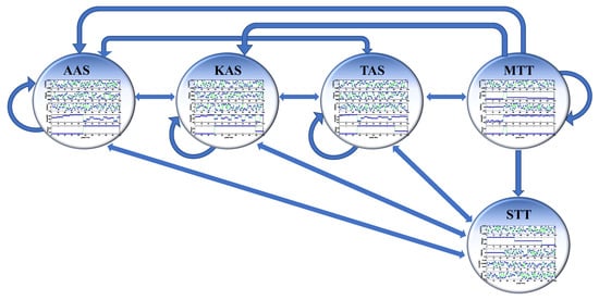
Figure 1.
Diagram of MFR working mode conversion.
We model the signal intelligence process of MFR from the perspective of the reconnaissance system. Figure 2 illustrates the geometric relationship between the reconnaissance system and the shipborne MFR. Antenna scanning methods significantly differ among various working modes. For instance, the antenna scans more rapidly when in search mode, while in tracking mode, the main beam of the antenna will gaze at the target location. The angle between the main lobe of the radar and the line of sight of the reconnaissance system is . The reconnaissance system antenna main lobe is always aimed at the target MFR. The distance between the reconnaissance system and the MFR is , and the reconnaissance system intercepts the radar power changes as shown in Equation (1). The change in directly affects the amplitude .
where represents the radar transmitting power, represents the radar antenna gain in the direction of the line of sight of the reconnaissance system, represents the signal wavelength, represents the main lobe gain of the receiving antenna of the reconnaissance system, and represents the feed loss and atmospheric loss.
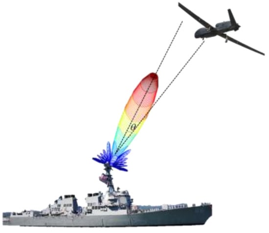
Figure 2.
Geometric relationship of reconnaissance scene.
Assuming that the sorting process has been completed, the intercepted radar signals all belong to the target MFR. The intercepted radar PDWs are denoted as , which includes the pulse arrival time, pulse width, carrier frequency, bandwidth and amplitude, etc., namely . The sequence of intercepted PDWs by the reconnaissance system can be represented as , and the input for work mode recognition can be described in array form as shown in Equation (2).
Ideally, the intercepted pulse data are complete, and the pulse repetition interval (PRI) of the pulse can be extracted from the PDWs. Taking the arrival time of the first pulse as time 0, the PRI of k-th pulses can be obtained by the difference between the arrival time of k+1-th pulses and the arrival time of k-th pulses, namely , where represents the total number of pulses obtained during the reconnaissance. Obviously, PRI is most sensitive to the change in the timing relationship.
In actual reconnaissance processes, the radar antenna scans in different directions during the detection process, combined with the influence of a complex electromagnetic environment. As a result, the reconnaissance pulse experiences phenomena such as deteriorating signal-to-noise ratio (SNR), multipath, and pulse splitting, leading to some missing or spurious pulses being inevitably lost, which disrupts the pulse temporal characteristics. In other words, the observed PDWs are incomplete, as shown in the following equation:
where represents the ascending order of the PDWs, represents all the real PDWs belonging to the target MFR under the ideal condition, represents the missing PDWs during reconnaissance, and represents the spurious PDWs generated during the reconnaissance. The mathematical model of the pulse temporal distribution with missing and spurious pulses is illustrated in Figure 3 and Figure 4. The orange and blue boxes represent pulse signals in two different working modes, while the dotted box in Figure 3 and Figure 4 respectively represents the effects of missing pulses and spurious pulses.
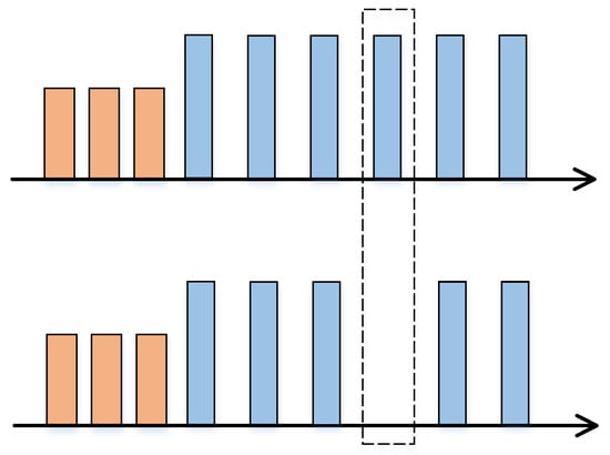
Figure 3.
Schematic diagrams of missing PDWs.
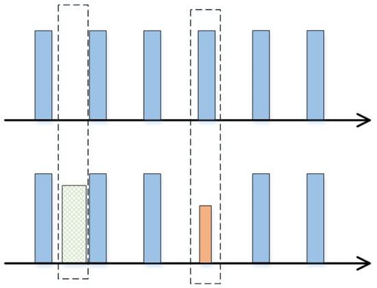
Figure 4.
Schematic diagrams of spurious PDWs.
Missing pulse and spurious pulse rate are defined as Equations (4) and (5), respectively.
where is the total number of real PDWs, is the number of missing PDWs, and is the number of spurious PDWs. In the case of missing pulses, the total number of samples will become . In the case of spurious pulses, the total number of samples will become .
Given a labeled dataset , we use it as a training set to train our model. consists of reconnaissance PDWs , with dimension , and corresponding sample labels , which belong to an output category space of dimension . Our goal is to design a function that is capable of correctly classifying an unknown sample into its corresponding working modes. The function must satisfy causal constraints and be a function of . The model should also prevent future information from leaking.
4. Dual-Path Time Convolution Attention Network
In response to the urgent need for MFR working mode recognition, this paper proposes a DP-ATCN-based MFR working mode recognition method inspired by TCN. Our goal is to learn a mapping function from PDWs to MFR working modes that can correctly classify unknown new samples into corresponding modes.
4.1. Introduction of Overall Network Structure
The overall structure of the MFR working mode recognition method based on DP-ATCN is illustrated in Figure 5. It consists of two modules: the SDR-DP-ATCN-based pre-recognition module (PRM) and the long PDW slice working mode secondary correction module (SCM). The intuition behind this method is to segment the radar PDWs into smaller blocks in time and obtain the pre-recognition results through SDR-DP-ATCN. When the reconnaissance system receives sufficient PDWs, the output feature vector after the fully connected layer is arranged in chronological order and input into the SCM to obtain the corrected working mode recognition results. This method adopts an end-to-end approach, where the PDWs are fed into the network to automatically extract features and achieve MFR working mode recognition.

Figure 5.
Structure of MFR working mode recognition method based on SDR-DP-ATCN.
4.2. Pre-Recognition Module Based on SDR-DP-ATCN
The MFR temporal feature mining and pre-recognition module consists of two parallel TCNs. Each TCN is composed of stacked residual modules [36,37]. To enhance the robustness and generalization ability of the network, ShakeDrop regularization is introduced to perform random shaking operations on certain layers in the network, allowing for more comprehensive information exchange between different network structures for the same input. At the same time, a CBAM is added to one path of the TCNs. CBAM helps the TCN to achieve adaptive feature importance screening, effectively reducing unnecessary information transmission and focusing on the most critical parts for classification. Additionally, because the CBAM attention module is a neuron unit that can be trained end-to-end, it can learn high-level feature representations to evaluate the interdependence between features, greatly improving the accuracy of time series data classification. Finally, the results of the two TCNs are concatenated and input into the cascaded fully connected layer, and the recognition results are obtained through softmax. The specific structure is shown in Figure 6.

Figure 6.
Diagram of MFR working mode pre-recognition module base on SDR-DP-ATCN.
During the PRM, the PDWs of time steps represented by (where represents the PDW dimension) are mapped to the feature space after max-min normalization. The model parameters are optimized and updated through the cross-entropy loss, backpropagation algorithm, and gradient descent algorithm. Once the model is trained, it is saved for future use.
4.2.1. Temporal Feature Extraction Based on ShakeDrop-Regularized TCN
TCN is a novel method that applies the idea of convolutional neural networks to the processing of temporal data. It can extract the temporal features of each variable in multivariate time series data, as well as the latent features between different variables at the same time. Notably, TCN disregards the ordering relationships among variables, aligning with the inherent features of PDWs.
TCN is composed of multiple cascading residual modules, which can effectively avoid the problem of network degradation when the model depth increases. Figure 7 depicts the internal architecture of each residual module, which comprises dilated causal convolution, weight normalization (WN), ReLU activation function, and ShakeDrop regularization. A skip connection is added after every two convolution calculations to perform identity mapping. The output of the residual module is the sum of the convolution calculation result and the identity mapping value. To flexibly control the depth of feature maps, achieve cross-channel information combination, add non-linear features, and maintain consistency in dimension between the input of the residual unit and the output of the convolution , a 1 × 1 convolution kernel is added to the identity mapping. Figure 7 shows the detailed structure of each residual modulation, which consists of causal dilated convolution, weight normalization, ReLU activation function, and ShakeDrop regularization. Every two convolutional calculations are followed by an identity mapping operation. The output of the residual module is the sum of the convolution calculation result and the identity mapping value.
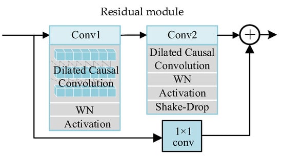
Figure 7.
Diagram of residual module.
We represent the input matrix of ResNet as , where . At each residual module, the output is expressed as
where is the output of the residual module, represents the mapping function, and denotes the overall representation after convolution, ReLU, and ShakeDrop. serves as the input of the next residual module.
The causal dilated convolution is a vital component in TCN, which can be divided into causal convolution and dilated convolution. For a 2D temporal input matrix and a convolutional kernel , the process of dilated causal convolution can be represented by Equation (7). The output at time is only dependent on the input in the interval of , ensuring that there is no leakage of future information in the hidden layers.
represents the result at position after one causal dilated convolution. represents the dilation factor, which is generally increased exponentially by powers of 2 as the convolutional layer changes, i.e., . is the size of the 1D convolutional kernel.
The convolutional receptive field of a network can be increased by increasing the size of the convolutional kernel, using a dilated convolution, and deepening the network. Such augmentations enable the convolution to extract more historical information, thereby enhancing the feature extraction performance of the network.
Weight normalization (WN) refers to the normalization of network weights . WN can accelerate convergence speed and stabilize the model training process. The WN method decouples weight into the product of length and direction , as shown in Equation (8),
where is a -dimensional vector, is a scalar, and is the L2 norm of .
The magnitude of the weight is normalized, and the normalized magnitude and direction are used to reconstruct the original weight
where is the normalized weight, is the magnitude of the original weight, and is the magnitude of the direction vector.
The Rectified Linear Unit (ReLU) activation function is a widely used non-linear activation function in deep neural networks. It has the advantage of simple computation, which can speed up the training and inference of the model, as shown in Equation (10).
The derivative of the ReLU is 0 when . This means that when the input is less than 0, the gradient of the ReLU is 0, which cannot update the parameters and may cause the “dying ReLU” problem. To solve the drawbacks, we use Leaky ReLU instead of ReLU, as shown in Equation (11).
The output of Leaky ReLU is . When , the output of Leaky ReLU is no longer 0, but a small negative number, which can effectively avoid the gradient of the network being 0. When , the output of the Leaky ReLU function is proportional to the input.
The challenge of labeling PDWs and scarce data creates a setback for working mode recognition of MFR. To regulate the network’s training to avoid overfitting, this paper proposes the incorporation of ShakeDrop regularization [38]. ShakeDrop rectifies the issue of unstable training while ensuring the effect of regularization. The purpose of introducing ShakeDrop aims to alleviate the problem of overfitting of ResNet. As the TCN network mainly consists of residual modules, it mainly benefits from this regularization method. The experimental results show that ShakeDrop has a constructive impact on the recognition of MFR working modes based on SDR-DP-ATCN.
The output of the -th residual modules after ShakeDrop is shown in Equation (12),
where and follow a uniform distribution on the interval [−1, 1] and [0, 1], respectively, and follows a Bernoulli distribution with probability , namely, . is determined by linear decay method, and the calculation formula is as follows:
where is an initial parameter, generally taking a value of 0.5.
During the training stage, the forward propagation process changes the weight of each branch, that is, it changes the impact of each branch on the final result, which can be understood as data augmentation. When backward propagation is performed, different random weight values are multiplied to interfere with the parameter updating, thereby avoiding the parameter becoming stuck in local optima [37]. controls the properties of ShakeDrop. When , ShakeDrop becomes the original residual network, promoting the network’s learning forward and producing an output, as shown in Equation (14).
When , ShakeDrop becomes Single-branch Shake, introducing interference to the network’s learning and producing an output as shown in Equation (15).
Using only Single-branch Shake did not perform well in experiments, mainly because the perturbation was too strong and lacked a stable mechanism. However, simply reducing the perturbation will weaken the effect of regularization. ShakeDrop takes from the Random Drop mechanism to achieve stable learning under strong perturbation, ensuring the regularization effect while overcoming the problem of unstable training.
In summary, the function mapping process of TCN of path 1 is shown in Equation (16).
4.2.2. Feature Extraction Based on CBAM
The Convolutional Block Attention Module (CBAM) helps the model to direct its focus to the relevant features, thereby enhancing its accuracy and performance. It comprises two sub-modules, namely, the Channel Attention Module (CAM) and the Spatial Attention Module (SAM). The CAM is responsible for weighting the feature maps of individual channels, allowing the model to focus on useful elements while discarding irrelevant and noisy features. The SAM, on the other hand, assigns weights to each spatial position of the feature map, permitting the model to emphasize significant feature regions while ignoring insignificant regions. Considering the influence that diverse feature channels and spatial information have on the recognition results of MFR working modes, this paper employs SDR-DP-ATCN, where a CBAM module is added to one of its paths to obtain attention weights on the channel and spatial dimensions. This method considerably elevates the correlation of features in the channel and spatial dimensions, making it more favorable for extracting efficient features of the MFR working modes. Following this, the PDW features of the CBAM are passed through a TCN module for further extraction of hidden features.
The CAM maintains the channel dimensions and compresses the spatial dimensions to obtain the importance weight of each channel. The input feature of this module is the normalized PDWs . First, the spatial dimensions of the input feature are separately subjected to global max pooling and global average pooling. Compared to using only one pooling, performing both global max pooling and global average pooling can obtain more feature information, resulting in two feature maps with a dimension of . They are then fed into a shared multi-layer perceptron (MLP), which consists of two fully connected layers and the ReLU activation function. The purpose of MLP is to compress the number of channels to , where is the reduction rate, and then expand it to the original number of channels. The two output features obtained are added together, and the final channel attention weight is generated by passing through the sigmoid activation function. is used to distinguish the importance of different channel features, and the calculation process is shown in the following equation.
where represents the input feature map, represents the global average pooling operation, represents the global max pooling operation, represents the multi-layer perceptron, and represents the sigmoid function.
Performing multiplication between the channel attention feature map and each channel of the original feature map results in a feature map that has been recalibrated based on channel features. The calculation formula is shown in the following equation:
where represents element multiplication operation.
For the input PDWs in this paper, each channel is a one-dimensional time series, which can be regarded as a spatial feature with a dimension of , , i.e., with a height of . Therefore, in this paper, the SAM focuses on which moment of data is more important for discriminating the current working mode.
The feature after passing through CAM is input into the SAM, where global max pooling and global average pooling are performed in the channel dimension. The two feature maps are then concatenated to obtain the feature dimension . The information at different positions is encoded and fused through convolutional operation with a kernel size of . The final spatial attention weight is obtained through the sigmoid function, as shown in the following equation.
Multiplying it with the input of this module results in the feature after passing through the CBAM module, as shown in the following equation.
Then, is fed into the TCN network in path 2 to obtain the temporal features, as shown in the following equation.
4.2.3. Feature Aggregation and Pre-Recognition Module
The output features from the SDR-DP-ATCNs are concatenated to form a new feature matrix , which is passed to the fully connected layer. In the fully connected layer, all nodes are connected to all nodes in the upper layer through weight values, which can integrate information with class discrimination in the features and map the high-dimensional distributed features extracted by the previous network structure to the sample label space. Two fully connected layers are adopted in this section, which can better solve nonlinear problems compared to a single fully connected layer. The fully connected layer is expressed by the following equation:
where is the transformation feature, and and are the weight and bias of the FC layer, respectively.
We utilize softmax regression to map the output of the fully connected layer to the interval , obtaining the classification result of the MFR. The calculation formula is shown below:
where is the probability of sample being classified into the class, and there are classes in total.
Through this series of processing, we obtain the predicted output of the PRM for short-temporal PDWs, as shown in the following formula.
where .
4.3. The Secondary Correction Module
The PDW of a multi-function radar intercepted by the reconnaissance system is a real-time data stream that transmits data packets. The pulse PDWs at each instant form a sequence that is fed sequentially into the working mode recognition network. To uphold the recognition’s real-time performance, the reconnaissance system must deliver swift feedback on the recognition results to the next module. Consequently, the aircraft cannot exclusively accumulate the pulse stream over an extended period to produce output results.
In the test stage, a constraint has to be implemented on the input sample’s length to the network. However, if the sample length is too short, there arises an issue of insufficient reliable historical information, which commonly leads to an increase in the error rate of the working mode recognition. Particularly, for the Track-While-Scan (TWS) mode that has both searching and tracking tasks, selecting an inadequate sample length could cause misjudgment. Therefore, to meet both the real-time requirements and network accuracy necessities, this paper proposes a secondary correction network to rectify the pre-prediction outcomes of the SDR-DP-ATCN pre-recognition module.
During the real-time reconnaissance process, PDWs divide the received pulse sequence into segments of length and input them into the DP-TCN preprocessing and network. If the overall length of the intercepted pulse sequence is relatively short, the recognition result of the pre-recognition network is directly used as the final result. When a certain number of pulses is accumulated, the preprocessing module outputs from historical moments are passed to the SCM of the results to obtain the final recognition result, namely, the input of SCM is . Here, the SCM adopts a single-layer TCN structure, and the final radar working mode recognition result is obtained through softmax layer output, .
4.4. Loss Function
The loss function for the model is defined as the cross-entropy between the true MFR working mode and the predicted class. The equation for the loss function is:
where represents the number of MFR working modes, represents the true label of the -th class in the -th sample, represents the predicted result of the model, and represents the number of samples. The model parameters are optimized iteratively using backpropagation and the training set.
When the loss reaches the set requirement or the maximum number of iterations is reached, the training of the network is completed. The radar PDW data are input into the pre-recognition module based on ATCN’s work mode temporal feature mining, which has been trained, to obtain preliminary radar work mode recognition results.
In the testing phase, the purpose of the model is to find the prediction result with the highest probability.
The weight update formula for a certain layer in the DP-ATCN is:
where represents the updated weight value of a certain layer, represents the current weight value of the layer, represents the learning rate, and represents the derivative of the loss function with respect to the current layer weight, which is also known as the gradient. The backpropagation algorithm updates weights layer by layer from the output layer to the input layer by computing the gradients of each layer in order to minimize the loss function.
5. Experiment
5.1. Data Set Introduction
In this paper, experiments and analyses were conducted to demonstrate the superiority and stability of the proposed algorithm, using the AN/SPY-1 shipborne MFR parameters as an example. Specifically, five typical operating modes of shipborne MFR were selected, including all-round area search (AAS), key area search (KAS), tracking and searching (TAS), multiple target tracking (MTT), and single target tracking (STT), to generate a pulse descriptor word (PDW) data stream simulation. The PDW stream consists of five dimensional features, including pulse carrier frequency (RF), pulse width (PW), pulse repetition interval (PRI), signal bandwidth (B), and signal amplitude (PA), with specific parameters provided in Table 1.

Table 1.
Parameters of MFR PDW.
To account for the difference in data rates for different working modes, each mode’s duration was designed to be between 0.5 and 1 s. The PDW switching rules for different working modes are shown in Figure 1 resulting in 120,000 PDWs arranged in order of TOA, with 30,000 pulse descriptor words per class. Each sample contains 64 time steps of PDWs, with a sample dimension of 64 × 5. The training set and test set were established at a ratio of 7:3, with a total of 1312 training samples and 562 test samples.
5.2. Training Settings
The experimental platform was constructed using the Win11 operating system and equipped with an Intel(R) Core(TM) i5-12400F 2.50GHz CPU and an NVIDIA GeForce RTX 3060 graphics card. Network framework construction relied on the integrated development environment PyCharm, utilizing PyTorch. During the training stage, the proposed network is optimized using backpropagation to compute the cross-entropy loss function. All network hyperparameters are listed in Table 2. It shows the specific network structure constructed in this section, including the number of cascaded residual blocks in each TCN module, and the use of ShakeDrop to connect residual blocks to improve network robustness and prevent overfitting. The input sample dimension for the pre-recognition network is set to 64, and the result-corrected network sample length is set to 6. The accuracy and loss curves for MFR working mode recognition during the training stage are presented in Figure 8. After 80 training epochs, the results become stable with an accuracy rate of 98.56%.

Table 2.
The Proposed Method’s Structure and Training Parameter Settings.
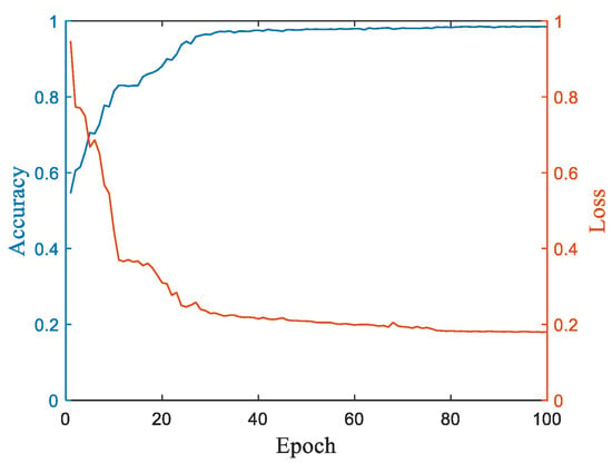
Figure 8.
Accuracy and loss curve during the training stage.
5.3. Test Results
During the test stage, the network parameters were fixed and the test data were inputted into the network to obtain recognition results. As shown in Figure 9, the test accuracy reaches 97.84%. It can be observed that the AAS, KAS, STT, and MTT modes’ recognition accuracy is all above 99%. The TAS shows the primary error, as it is confused with the standalone search or tracking mode, which is consistent with the theory. The experimental results demonstrate that the proposed method is feasible and effective for recognizing MFR working modes.
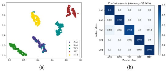
Figure 9.
Test Results. (a) T-SNE visualization; (b) confusion matrix.
5.4. Ablation Study
In order to validate the effectiveness of the MFR working mode recognition algorithm based on DP-ATCN proposed in this paper, this section conducts experiments to assess the impact of the dual-path structure, attention module, ShakeDrop regularization, and result correction module on recognition accuracy. All experiments utilize the same training and testing sets to ensure fairness.
Experiment 1 serves as a control and employs the DP-ATCN model proposed in this paper. In Experiment 2, the dual-path model is not used, and instead, the attention module and the three TCN network layers are directly cascaded. Experiment 3 removes the attention module from DP-ATCN while keeping the other components unchanged. Experiment 4 replaces ShakeDrop regularization with the basic Dropout module. Experiment 5 excludes the result correction module. To facilitate effective comparison, the sample length is maintained at 64 × 6, which corresponds to the overall length of multiple samples that can undergo mode correction. In Experiment 6, the basic TCN model with three cascaded TCN layers is employed, and the sample length is 64 × 6.
As shown in Table 3, “√” represents the inclusion of a module, while “×” represents the deletion of that module. the experimental results demonstrate that each module or structure added in this paper has a positive effect on the overall radar mode recognition performance of the network, which proves the necessity of each module and the effectiveness of the entire network for recognition.

Table 3.
Ablation Experimental Results.
5.5. Comparison of the Proposed Method with Other Algorithms
This section compares the effectiveness of the CNN, the HSSLSTM [19], the GRU [31], and the proposed DP-ATCN-based MFR working mode recognition algorithm. The test accuracy of the four comparison networks and the proposed network is shown in Table 4. The first and second columns of Figure 10 show the T-SNE visualization results and confusion matrix of the four algorithms, respectively. It can be seen that for the sequence data of multi-function radar pulses, the CNN network has poor recognition performance. The proposed DP-ATCN-based recognition algorithm can better distinguish inter-class features and achieve better recognition performance compared to other methods.

Table 4.
Different network test accuracy.

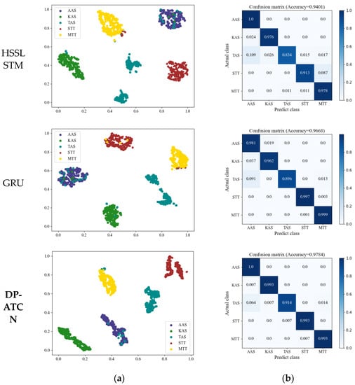
Figure 10.
Comparison of the T-SNE visualization and confusion matrix between CNN HSSLSTM, GRU, and the proposed DP-ATCN. (a) T-SNE visualization; (b) confusion matrix.
Here, we randomly introduced 5–50% spurious and missing PDWs into the reconnaissance PDWs to test the generalization and stability of the method proposed in this paper and compared the performance with three other network models mentioned above. From the experimental results shown in Figure 11, as the reconnaissance environment deteriorates, the test accuracy of all algorithms will decrease, which is expected. However, the proposed method in this paper still has better recognition ability compared to the others. When there are 20% spurious and missing PDWs, the recognition accuracy based on DP-ATCN can still reach around 80%, which indicates that the method proposed in this article has a certain degree of robustness and generalization ability to noise and interference.
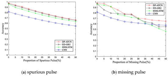
Figure 11.
Recognition results with the change in (a) spurious pulse rate and (b) missing pulse rate.
6. Conclusions
This article proposes a long time series feature-preserving MFR working mode recognition method based on DP-ATCN. The method fully considers the temporal correlation between radar reconnaissance PDWs, adopts a dual-path structure, and introduces CBAM and ShakeDrop-regularization modules to extract temporal features, obtaining high-dimensional space mapping of PDW features within a short time slice. With the accumulation of PDWs over time, an enhanced TCN network is introduced to obtain the time-varying characteristics of long-term dependencies, achieving timely and accurate secondary correction of the radar operational mode recognition results. Finally, the stability and superiority of the proposed algorithm are verified under five typical operational modes of shipborne MFR. The necessity of each module is verified through ablation experiments. The experimental results show that under complex electromagnetic environments such as spurious and missing PDWs, the proposed algorithm can effectively extract the temporal differences between different working modes and distinguish different operational modes, and it has certain superiority.
Author Contributions
Conceptualization, T.T.; Methodology, T.T.; Validation, Q.Z.; Investigation, Q.Z. and X.G.; Resources, Z.Z.; Data curation, F.N.; Writing—original draft, T.T.; Writing—review & editing, T.T.; Funding acquisition, F.Z. All authors have read and agreed to the published version of the manuscript.
Funding
This work was supported in part by the National Natural Science Foundation of China under Grant 62101412, Grant 62001350; in part by the Fundamental Research Funds for the Central Universities under Grant ZYTS23146; in part by the China Postdoctoral Science Foundation under Grant 2020M673346; in part by the Joint Fund of Ministry of Education under Grant 6141A02022367.
Data Availability Statement
Not applicable.
Conflicts of Interest
The authors declare no conflict of interest.
References
- Weber, M.E.; Cho, J.Y.N.; Thomas, H.G. Command and Control for Multifunction Phased Array Radar. IEEE Trans. Geosci. Remote Sens. 2017, 55, 5899–5912. [Google Scholar] [CrossRef]
- Li, Z.; Perera, S.; Zhang, Y.; Zhang, G.; Doviak, R. Phased-Array Radar System Simulator (PASIM): Development and Simulation Result Assessment. Remote Sens. 2019, 11, 422. [Google Scholar] [CrossRef]
- Stailey, J.E.; Hondl, K.D. Multifunction Phased Array Radar for Aircraft and Weather Surveillance. Proc. IEEE 2016, 104, 649–659. [Google Scholar] [CrossRef]
- Haigh, K.; Andrusenko, J. Cognitive Electronic Warfare: An Artificial Intelligence Approach; Artech: Morristown, NJ, USA, 2021; Available online: http://ieeexplore.ieee.org/document/9538834 (accessed on 1 September 2021).
- Gurbuz, S.Z.; Griffiths, H.D.; Charlish, A.; Rangaswamy, M.; Greco, M.S.; Bell, K. An Overview of Cognitive Radar: Past, Present, And Future. IEEE Aerosp. Electron. Syst. Mag. 2019, 34, 6–18. [Google Scholar] [CrossRef]
- Butler, J. Tracking and Control in Multi-Function Radar. Ph.D. Thesis, University of London, London, UK, 1998. [Google Scholar]
- Zhai, Q.; Li, Y.; Zhang, Z.; Li, Y.; Wang, S. Few-Shot Recognition of Multi-Function Radar Modes via Refined Prototypical Random Walk Network. IEEE Trans. Aerosp. Electron. Syst. 2022, 59, 2376–2387. [Google Scholar] [CrossRef]
- Maini, A.M. Handbook of Defence Electronics and Optronics: Fundamentals, Technologies and Systems; Wiley: Hoboken, NJ, USA, 2018. [Google Scholar]
- Ou, J.; Zhao, F.; Ai, X.; Yang, J.; Chen, Y. Data-Driven Method of Reverse Modelling for Multi-Function Radar. In Proceedings of the 2017 25th European Signal Processing Conference (EUSIPCO), Kos, Greece, 28 August–2 September 2017; pp. 1947–1951. [Google Scholar]
- Arasaratnam, I.; Haykin, S.; Kirubarajan, T.; Dilkes, F. Tracking the Mode of Operation of Multi-Function Radars. In Proceedings of the 2006 IEEE Conference on Radar, Verona, NY, USA, 24–27 April 2006; pp. 6–11. [Google Scholar]
- Chen, H.; Feng, K.; Kong, Y.; Zhang, L.; Yu, X.; Yi, W. Function Recognition of Multi-Function Radar Via CNN-GRU Neural Network. In Proceedings of the 2022 23th International Radar Symposium (IPS), Gdansk, Poland, 12–14 September 2022; pp. 71–76. [Google Scholar]
- Zhang, Z.; Li, Y.; Zhai, Q.; Li, Y.; Gao, M. Mode Recognition of Multifunction Radars for Few-Shot Learning Based on Compound Alignments. IEEE Trans. Aerosp. Electron. Syst. 2022, 58, 5860–5874. [Google Scholar] [CrossRef]
- Wang, A.; Krishnamurthy, V. Threat Estimation of Multifunction Radars: Modeling and Statistical Signal Processing of Stochastic Context Free Grammars. In Proceedings of the 2007 IEEE International Conference on Acoustics, Speech and Signal Processing—ICASSP, Honolulu, HI, USA, 15–20 April 2007; pp. III-793–III-796. [Google Scholar]
- Kauppi, J.-P.; Martikainen, K.; Ruotsalainen, U. Hierarchical Classification of Dynamically Varying Radar Pulse Repetition Interval Modulation Patterns. Neural Netw. 2010, 23, 1226–1237. [Google Scholar] [CrossRef]
- Ou, J.; Chen, Y.; Zhao, F.; Ai, X.; Yang, J. Research on Extension of Hierarchical Structure for Multifunction Radar Signals. In Proceedings of the 2017 Progress In Electromagnetics Research Symposium—Spring (PIERS), St. Petersburg, Russia, 22–25 May 2017; pp. 2612–2616. [Google Scholar]
- Revillon, G.; Mohammad-Djafari, A.; Enderli, C. Radar Emitters Classification and Clustering with a Scale Mixture of Normal Distributions. In Proceedings of the 2018 IEEE Radar Conference (RadarConf18), Oklahoma City, OK, USA, 23–27 April 2018; pp. 1371–1376. [Google Scholar]
- Visnevski, N. Syntactic Modeling of Multi-Function Radars. Ph.D. Thesis, University of McMaster, Hamilton, ON, Canada, 2005. [Google Scholar]
- Visnevski, N.; Krishnamurthy, V.; Wang, A.; Haykin, S. Syntactic Modeling and Signal Processing of Multifunction Radars: A Stochastic Context-Free Grammar Approach. Proc. IEEE 2007, 95, 1000–1025. [Google Scholar] [CrossRef]
- Li, Y.; Zhu, M.; Ma, Y.; Yang, J. Work Modes Recognition and Boundary Identification of MFR Pulse Sequences with a Hierarchical Seq2seq LSTM. IET Radar Sonar Navig. 2020, 14, 1343–1353. [Google Scholar] [CrossRef]
- Bai, S.; Kolter, J.Z.; Koltun, V. An Empirical Evaluation of Generic Convolutional and Recurrent Networks for Sequence Modeling. arXiv 2018, arXiv:1803.01271. [Google Scholar] [CrossRef]
- Wang, A.; Krishnamurthy, V. Signal Interpretation of Multi-Function Radars: Modeling and Statistical Signal Processing with Stochastic Context Free Grammar. IEEE Trans. Signal Process. 2008, 56, 1106–1119. [Google Scholar] [CrossRef]
- Wang, A.; Krishnamurthy, V. Modeling and Interpretation of Multifunction Radars with Stochastic Grammar. In Proceedings of the 2008 IEEE Aerospace Conference, Big Sky, MT, USA, 1–8 March 2008; pp. 1–13. [Google Scholar]
- Ou, J.; Chen, Y.; Zhao, F.; Li, C.; Xiao, S. Novel Approach for the Recognition and Prediction of Multi-Function Radar Behaviours Based on Predictive State Representations. Sensors 2017, 17, 632. [Google Scholar] [CrossRef]
- Ou, J.; Chen, Y.; Zhao, F.; Liu, J.; Xiao, S. Method for Operating Mode Identification of Multi-Function Radars Based on Predictive State Representations. IET Radar Sonar Navig. 2017, 11, 426–433. [Google Scholar] [CrossRef]
- Xiong, J.; Pan, J.; Zhuo, Y.; Guo, L. Airborne Multi-function Radar Air-to-air Working Pattern Recognition Based on Bayes Inference and SVM. In Proceedings of the 2022 5th International Conference on Information Communication and Signal Processing (ICICSP), Shenzhen, China, 26–28 November 2022; pp. 622–629. [Google Scholar]
- Wang, L.; Yang, X.Y.; Tan, H.Y.; Bai, X.; Zhou, F. Few-Shot Class-Incremental SAR Target Recognition Based on Hierarchical Embedding and Incremental Evolutionary Network. IEEE Trans. Geosci. Remote Sens. 2023, 61, 5204111. [Google Scholar] [CrossRef]
- Geng, J.; Wang, H.Y.; Fan, J.C.; Ma, X. SAR Image Classification via Deep Recurrent Encoding Neural Networks. IEEE Trans. Geosci. Remote Sens. 2018, 56, 2255–2269. [Google Scholar] [CrossRef]
- Liu, Z.; Yu, P. Classification, Denoising and Deinterleaving of Pulse Streams with Recurrent Neural Networks. IEEE Trans. Aerosp. Electron. Syst. 2019, 55, 1624–1639. [Google Scholar] [CrossRef]
- Li, X.Q.; Liu, Z.M.; Huang, Z.T.; Liu, W. Radar Emitter Classification with Attention-based Multi-RNNs. IEEE Commun. Lett. 2020, 24, 2000–2004. [Google Scholar] [CrossRef]
- Xu, X.; Bi, D.; Pan, J. Method for Functional State Recognition of Multifunction Radars Based on Recurrent Neural Networks. IET Radar Sonar Navig. 2021, 15, 724–732. [Google Scholar] [CrossRef]
- Chen, H.; Feng, K.; Kong, Y.; Zhang, L.; Yu, X.; Yi, W. Multi-Function Radar Work Mode Recognition Based on Encoder-Decoder Model. In Proceedings of the IGARSS 2022-2022 IEEE International Geoscience and Remote Sensing Symposium, Kuala Lumpur, Malaysia, 17–22 July 2022; pp. 1189–1192. [Google Scholar]
- Liu, Z.M. Recognition of Multifunction Radars via Hierarchically Mining and Exploiting Pulse Group Patterns. IEEE Trans. Aerosp. Electron. Syst. 2020, 56, 4659–4672. [Google Scholar] [CrossRef]
- Feng, K.G.; Chen, H.Y.; Kong, Y.K.; Zhang, L.; Yu, X.; Yi, W. Prediction of Multi-Function Radar Signal Sequence Using Encoder-Decoder Structure. In Proceedings of the 2022 7th International Conference on Signal and Image Processing (ICSIP), Suzhou, China, 20–22 July 2022; pp. 152–156. [Google Scholar]
- Zhang, Z.; Li, Y.; Zhai, Q.; Li, Y.; Gao, M. Few-shot Learning for Fine-Grained Signal Modulation Recognition based on Foreground Segmentation. IEEE Trans. Veh. Technol. 2022, 71, 2281–2292. [Google Scholar] [CrossRef]
- Khandelwal, U.; He, H.; Qi, P.; Jurafsky, D. Sharp Nearby, Fuzzy Far Away: How Neural Language Models Use Context. In Proceedings of the 56th Annual Meeting of the Association for Computational Linguistics (ACL 2018), Melbourne, Australia, 15–20 July 2018; pp. 284–294. [Google Scholar]
- Huang, G.; Sun, Y.; Liu, Z.; Sedra, D.; Weinberger, K.Q. Deep Networks with Stochastic Depth. In Proceedings of the Computer Vision-ECCV 2016, Amsterdam, The Netherlands, 11–14 October 2016; pp. 646–661. [Google Scholar]
- Kleinberg, R.; Li, Y.; Yuan, Y. An Alternative View: When Does SGD Escape Local Minima? In Proceedings of the 35th International Conference on Machine Learning, Stockholm, Sweden, 10–15 July 2018; pp. 2698–2707. [Google Scholar]
- Yamada, Y.; Iwamura, M.; Akiba, T.; Kise, K. Shakedrop Regularization for Deep Residual Learning. IEEE Access 2019, 7, 186126–186136. [Google Scholar] [CrossRef]
Disclaimer/Publisher’s Note: The statements, opinions and data contained in all publications are solely those of the individual author(s) and contributor(s) and not of MDPI and/or the editor(s). MDPI and/or the editor(s) disclaim responsibility for any injury to people or property resulting from any ideas, methods, instructions or products referred to in the content. |
© 2023 by the authors. Licensee MDPI, Basel, Switzerland. This article is an open access article distributed under the terms and conditions of the Creative Commons Attribution (CC BY) license (https://creativecommons.org/licenses/by/4.0/).