Removing Moving Objects without Registration from 3D LiDAR Data Using Range Flow Coupled with IMU Measurements

Abstract

Removing moving objects from 3D LiDAR data plays a crucial role in advancing real-time odometry, life-long SLAM, and motion planning for robust autonomous navigation. In this paper, we present a novel method aimed at addressing the challenges faced by existing approaches when dealing with scenarios involving significant registration errors. The proposed approach offers a unique solution for removing moving objects without the need for registration, leveraging range flow estimation combined with IMU measurements. To this end, our method performs global range flow estimation by utilizing geometric constraints based on the spatio-temporal gradient information derived from the range image, and we introduce IMU measurements to further enhance the accuracy of range flow estimation. Through extensive quantitative evaluations, our approach showcases an improved performance, with an average mIoU of 45.8%, surpassing baseline methods such as Removert (43.2%) and Peopleremover (32.2%). Specifically, it exhibits a substantial improvement in scenarios characterized by a deterioration in registration performance. Moreover, our method does not rely on costly annotations, which make it suitable for SLAM systems with different sensor setups.

1. Introduction

Moving objects removal from 3D laser scan data is a crucial task for simultaneous localization and mapping (SLAM) in autonomous navigation [1,2,3,4]. Laser scans data from dynamic scenes often contain a large number of points belonging to moving objects, such as vehicles. The purpose of moving object removal is to distinguish these dynamic points from static background points. There are two principal reasons for removing moving objects points. First, a high proportion of moving object points can have detrimental effects on LiDAR odometry performance and potentially lead to SLAM failure in real-world environments [5,6]. Additionally, for generating long-term static maps, it is imperative to remove the aggregated dynamic points, which are called “long tails or ghost”, from the point cloud data [2,7,8]. Numerous innovative approaches have been proposed to tackle this issue, categorizing them into three main groups: comparison after registration, segmentation based on learning, and scene-flow-based methods. We have compiled a list of representative methods for each category, which are presented for comparison in Table 1.

Comparison after registration. The first category of methods, which is the most commonly used, follows a pipeline that begins with the spatial registration of laser scans, subsequent conversion of these scans into an occupancy grid map, and finally identification of grids that contain moving objects based on noticeable differences between current and reference scans (e.g., [2,4,9,10]). These methods successfully detected moving objects based on the assumption that the current and reference scans can be aligned perfectly [9]. Unfortunately, the presence of moving objects, particularly large buses and trucks, can introduce challenges in accurately aligning the scans in terms of translation and rotation. This can subsequently lead to failures in removing moving objects. Therefore, it becomes imperative to address the removal of moving objects prior to LiDAR registration to ensure more reliable and accurate results.

Segmentation based on learning. The second category of methods focuses on removing dynamic objects through semantic segmentation. Recent advancements in deep-learning-based approaches, such as LMNet [1], have shown promising results in terms of detection accuracy [11,12,13,14,15,16]. These methods leverage multi-scans as input data and do not rely on LiDAR registration, offering a more efficient and effective solution. Nevertheless, these methods heavily depend on a substantial amount of training labels, which can be costly to acquire and limited in availability. Currently, the SemanticKITTI [1] dataset is the primary source for such labels, making it challenging to adapt these methods to other scenarios with different sensor setups. While several unsupervised techniques, such as MOTS [14], have attempted to address this issue, they typically rely on GPUs for efficient computation. However, the lack of GPU availability in many practical SLAM systems poses a challenge for implementing these methods effectively.

Scene-flow-based methods. LiDAR scene flow estimation involves estimating the 3D structure and 3D motion of individual points within moving point clouds [17,18,19]. The pioneering learning-based network, FlowNet3D [18], directly estimates scene flow from point clouds. However, annotating LiDAR scene flow is a highly challenging task. To overcome this challenge, SLIM [19] introduces self-supervised training techniques to enhance flow prediction without the need for extensive manual annotation. Overall, the field of LiDAR scene flow estimation is expected to advance further in terms of computational efficiency and prediction accuracy.

Table 1. A summary of different methods.

Methods	Relying on Registration	Using Training Labels	Using GPUs
ERASOR [2]	✔	✘	✘
Peopleremover [4]	✔	✘	✘
Mapless [9]	✔	✘	✘
Removert [10]	✔	✘	✘
LMNet [1]	✘	✔	✔
MOTS [14]	✘	✘	✔
FlowNet3D [18]	✘	✔	✔
SLIM [19]	✘	✘	✔
Proposed	✘	✘	✘

Table 1. A summary of different methods.

Methods	Relying on Registration	Using Training Labels	Using GPUs
ERASOR [2]	✔	✘	✘
Peopleremover [4]	✔	✘	✘
Mapless [9]	✔	✘	✘
Removert [10]	✔	✘	✘
LMNet [1]	✘	✔	✔
MOTS [14]	✘	✘	✔
FlowNet3D [18]	✘	✔	✔
SLIM [19]	✘	✘	✔
Proposed	✘	✘	✘

In this study, we focus on techniques that can identify moving objects without the need for registration between consecutive laser scans. We aim to achieve this without relying on annotated labels or GPUs in order to explore SLAM approaches that are not reliant on data-driven methods like LOAMs [20]. One potential solution to this problem is to transform laser scans into 2D range images, rather than 3D point clouds, and then use 2D optical flow to detect the moving objects. However, applying optical flow to our case poses a challenge because of the violation of the assumption that the intensity of objects remains constant over time, which is not satisfied for range images [21,22]. Hence, we propose a novel method to remove the moving objects from sequential 3D laser scans. Our approach considers a geometric constraint based on the spatial–temporal gradient of the range image to identify moving objects prior to registration.

To the best of our knowledge, no existing approach has yet incorporated a dense range-based geometric constraint for the removal of moving objects in the domain of 3D point clouds. The proposed method is evaluated using three datasets, namely the publicly accessible dataset SemanticKITTI, along with two additional datasets recorded from open urban scenarios involving large vehicles. Figure 1 exemplifies the successful identification of a moving vehicle using our method based on two consecutive scans. The main contributions of this paper are follows:

(1)

Proposing a novel method: we introduce a novel method for moving objects removal without registration by considering range geometric constraints and IMU measurements in a 3D point clouds domain.

(2)

Dataset evaluation: Our proposed method is evaluated on three datasets, and the experimental results demonstrate that it outperforms the baseline methods. Importantly, our method achieves this superior performance without relying on accurate LiDAR registration or expensive annotations. This characteristic makes our method highly suitable for integration with widely accessible SLAM systems.

2. Methods

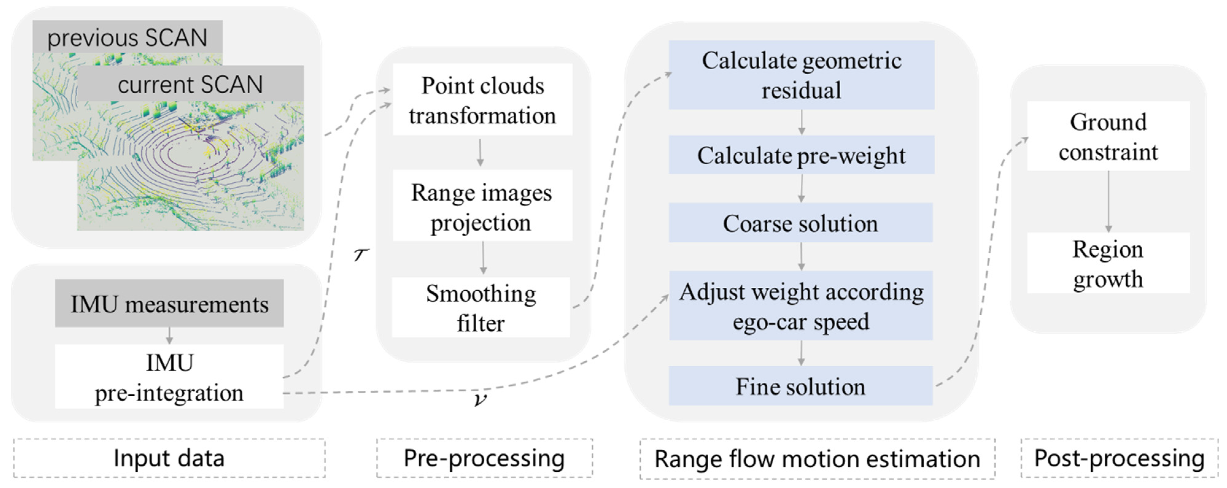
Many of the existing dynamic object removal methods focus on identifying local discrepancies between current and reference scans [2,9,10]. However, these approaches may encounter challenges in detecting moving objects when the LiDAR registration is not perfectly aligned. In this paper, our focus is on globally detecting moving objects (foreground) from the background without relying on LiDAR registration. We propose a novel pipeline for the removal of moving objects, which is based on range flow and incorporates IMU measurements. As illustrated in Figure 2, the proposed pipeline comprises three main stages: pre-processing, range flow motion estimation, and postprocessing. The proposed algorithm is described in Algorithm 1.

Algorithm 1: Moving Objects Removal without Registration

Input: $\mathrm{The} \mathrm{previous} \mathrm{scan} {\mathcal{S}}_1$$, \mathrm{the} \mathrm{current} \mathrm{scan} {\mathcal{S}}_2$; The prior pose between two scans from IMU measurements $\mathcal{T}$; The current speed of the ego-car from IMU measurements $\mathcal{V}$.

Pre-processing: 1. Coarsely align scan ${\mathcal{S}}_1$ to scan ${\mathcal{S}}_2$ based on transformation $\mathcal{T}$$\Rightarrow$ ${\mathcal{S}}_1^t$,${\mathcal{S}}_2$; 2. Perform range image projection and apply smoothing on scans ${\mathcal{S}}_1^t$,${\mathcal{S}}_2$$\Rightarrow$${\mathcal{I}}_1$, ${\mathcal{I}}_2$. Range flow estimation: 3. Compute the geometric constraint residual for each point using range images ${\mathcal{I}}_1$,${\mathcal{I}}_2$ $\Rightarrow$${\rho }_i(\xi )$; 4. Compute pre-weight of each point $\Rightarrow$$w_i$; 5. Obtain a coarse solution of range flow by minimizing the loss function $\mathcal{L}$$\Rightarrow$${\xi }^{*}(R^{\prime },{\omega }^{\prime },{\alpha }^{\prime })$; 6. Adjust the weight of each point by incorporating the ego-car speed $\mathcal{V}$$\Rightarrow$ $w^t{}_i$; 7. Obtain a fine solution by recomputing Step 6 with the adjusted weight $w^t{}_i$$\Rightarrow$$\xi (R^{\prime },{\omega }^{\prime },{\alpha }^{\prime })$; 8. Segment points belonging to moving objects according the fine range flow $\xi (R^{\prime },{\omega }^{\prime },{\alpha }^{\prime })$. Post-processing: 9. Perform ground removal and region growth techniques to improve the segmentation.

2.1. IMU Measurements

Traditional methods of removing moving objects that rely on registration techniques may struggle to handle scenarios involving large vehicles in point clouds. Therefore, to overcome this limitation, we propose the use of range flow, which is an approach similar to optical flow, to successfully remove moving objects. However, estimating range flow on laser scan data poses a challenge because of discontinuous gradients caused by the sparsity of points and noisy measurements.

The inertial measurement unit (IMU) sensor offers precise inertial data, including angular rate and specific force/acceleration, within a brief timeframe [23]. In autonomous driving, the integration of an IMU and global navigation satellite system (GNSS) is common for real-time localization and navigation [24,25]. Nevertheless, the utilization of IMU measurements for the removal of moving objects has been scarcely explored in previous studies. In this study, we leverage IMU measurements to assist in estimating range flow by utilizing IMU odometry and the speed of the ego-car.

These measurements serve as valuable inputs that aid in accurately estimating the range flow information. In optical flow, the pyramid strategy [26] is a commonly utilized approach to estimate large displacements. However, in our method, we leverage IMU odometry to achieve coarse alignment between two consecutive scans. This allows us to bypass the time-consuming pyramid strategy, resulting in more efficient processing. Additionally, the speed of the ego-car obtained from IMU measurements serves another crucial purpose of noise suppression. By leveraging the ego-car speed, we can effectively filter out noise points, thereby significantly enhancing the accuracy of range flow estimation. In this study, we employed the fourth order Runge-Kutta integration to discretize the IMU motion formula [27], allowing us to obtain IMU odometry and velocity.

2.2. Range Image Representation

Our approach places a strong emphasis on computational efficiency. The utilization of range images instead of 3D point clouds can avoid heavy computation compared to directly processing point clouds. By operating on range images, we can leverage fast algorithms commonly used for 2D images, such as filtering and ground segmentation techniques [28]. Spherical coordinate projection, as described in [10,29], is utilized to convert 3D point clouds from Cartesian coordinates $(x,y,z)$ to spherical coordinates $(R,\omega ,\alpha )$ (see Equations (1)–(3)). The range, elevation, and azimuth values are denoted as $R,\omega ,\alpha$. By resampling $R,\omega ,\alpha$, we can obtain the intensity, height, and width of the range image, respectively.

$$R=\sqrt{x^2+y^2+z^2}$$

(1)

$$\omega =\arcsin \frac{z}{R}$$

(2)

$$\alpha =\arctan \frac{x}{y}$$

(3)

2.3. Smoothing Filter

Gradient calculations serve as the foundation of range flow estimation. In order to improve the accuracy of range flow and to mitigate the effects of noise, it is essential to apply a smoothing filter to the range images. Choosing an appropriate gradient smoothing filtering algorithm is crucial for achieving this goal. In our study, we utilize the median filter for smoothing, as it has been shown to achieve better performance compared to other common filters such as bilateral and Gaussian filters. The median filter can effectively balance noise reduction and the preservation of details, making it a practical choice for our application.

2.4. Range Flow Estimation

As mentioned above, numerous methods relying on high-precision registration can fail to detect moving objects in scenarios where LiDAR registration becomes challenging because of the presence of these objects. In such cases, range flow estimation is considered a viable alternative for detecting moving objects without relying on registration techniques.

While motion estimation based on range flow draws inspiration from optical flow techniques, it differs from optical-flow-based methods because of the different types of information provided by the two image modalities [30]. In an optical image, pixel intensity represents the brightness of objects, while in a range image, the pixel’s intensity value represents the distance or depth of the object from the sensor. The optical-flow-based approach assumes that the brightness of the observed object points remains constant over time, which is not valid for range images.

In order to determine the range flow for individual pixels in a range image, the pixel’s motion is represented through spatial–temporal gradients. Spatial–temporal gradient information captures the changes in pixel values within both its spatial neighborhood (incorporating horizontal and vertical movements in the current range image) and its temporal neighborhood (examining two consecutive range images) over a specific time interval. Following that, we integrate a range-based geometric constraint, utilizing spatio-temporal gradient information, to address the range flow estimation of each pixel. Moreover, we make the underlying assumption that the motion of moving objects follows rigid motion principles.

2.4.1. 3D Range Flow Representation

Let $R(\omega ,\alpha ,t)$ be the representation of range magnitude of an individual point in a 3D spherical coordinate, and $\omega ,\alpha$ are, respectively, the azimuth and pitch angle of a point from the sensor origin at time $t$. Assuming $R(\omega ,\alpha ,t)$ is differentiable in a small displacement, the function of its first-order Taylor series expansion at time $t+dt$ can be expressed as follows:

$$R(\omega +d\omega ,\alpha +d\alpha ,t+dt)=R(\omega ,\alpha ,t)+\frac{\mathsf{\partial }R}{\mathsf{\partial }\omega }d\omega +\frac{\mathsf{\partial }R}{\mathsf{\partial }\alpha }d\alpha +\frac{\mathsf{\partial }R}{\mathsf{\partial }t}dt+O(\omega ,\alpha ,t)$$

(4)

where $O(\omega ,\alpha ,t)$ represents the second-order and higher-order terms.

By combining Equations (4)–(6), we can derive Equation (7), which represents the expression of range gradients when the sensor is moving during the time lapse $dt$. Equation (7) reflects the 3D range-based geometric constraint.

$$dR=R(\omega +d\omega ,\alpha +d\alpha ,t+dt)-R(\omega ,\alpha ,t)$$

(5)

$$\frac{dR}{dt}=\frac{\mathsf{\partial }R}{\mathsf{\partial }w}\frac{d\omega }{dt}+\frac{\mathsf{\partial }R}{\mathsf{\partial }\phi }\frac{d\alpha }{dt}+\frac{\mathsf{\partial }R}{\mathsf{\partial }t}$$

(6)

$$R^{\prime }={R^{\prime }}_{\omega }{\omega }^{\prime }+{R^{\prime }}_{\alpha }{\alpha }^{\prime }+{R^{\prime }}_t$$

(7)

with

$$\begin{array}{c}{R^{\prime }}_{\omega }=\frac{\mathsf{\partial }R}{\mathsf{\partial }\omega },{R^{\prime }}_{\alpha }=\frac{\mathsf{\partial }R}{\mathsf{\partial }\alpha },{R^{\prime }}_t=\frac{\mathsf{\partial }R}{\mathsf{\partial }t}\\ {\omega }^{\prime }=\frac{d\omega }{dt},{\alpha }^{\prime }=\frac{d\alpha }{dt}\end{array}$$

where $R^{\prime }$ represents the total derivative of range, while ${\omega }^{\prime }$ and ${\alpha }^{\prime }$ denote horizontal and vertical velocity flow of each point on current range image, respectively. The terms ${R^{\prime }}_{\omega },{R^{\prime }}_{\alpha }$, and ${R^{\prime }}_t$ denote the partial derivatives of the range with respect to azimuth $\omega$, pitch $\alpha$, and time $t$, respectively. $R^{\prime }$ can be calculated from the three partial derivatives ${R^{\prime }}_{\omega },{R^{\prime }}_{\alpha },{R^{\prime }}_t$ and velocity flow $({\omega }^{\prime },{\alpha }^{\prime })$. The three partial derivatives of range ${R^{\prime }}_{\omega },{R^{\prime }}_{\alpha },{R^{\prime }}_t$ are known and can be obtained directly from range images, while $R^{\prime }$ and velocity flow $({\omega }^{\prime },{\alpha }^{\prime })$ are unknown and need to be estimated.

2.4.2. Coarse Estimation of Range Flow

A dense function to motion estimation considering each pixel on range images is proposed in this part. For each pixel on a range image, we need to estimate the total derivative of range $R^{\prime }$ and the velocity of horizontal and vertical movement ${\omega }^{\prime },{\alpha }^{\prime }$. Let $\xi =(R^{\prime },{\omega }^{\prime },{\alpha }^{\prime })$ be the variable of range flow to be estimated and $\rho (\xi )$ in Equation (8) be geometric constraint residual for each pixel. Our objective is to globally estimate range flow $\xi$ for each point globally by minimizing the loss function $\mathcal{L}$ in Equation (9):

$$\rho (\xi )={R^{\prime }}_{\omega }{\omega }^{\prime }+{R^{\prime }}_{\alpha }{\alpha }^{\prime }+{R^{\prime }}_t-R^{\prime }$$

(8)

$$\mathcal{L}=\underset{\xi }{\arg \min }{\displaystyle \sum _{i=1}^N\mathcal{F}(w_i{\rho }_i(\xi ))})$$

(9)

with

$$\begin{array}{c}\mathcal{F}(\rho )=\frac{k^2}{2}\ln (1+{(\frac{\rho }{k})}^2)\\ w(\rho )=\frac{1}{1+k{\rho }^2}\end{array}$$

Here, we choose the Cauchy M-estimator as robust function $\mathcal{F}(•)$, which is similar to reference [31], and $w(\rho )$ is used to calculate the weight based on the geometric constraint residual for each point, and k is adjustable between 0 and 1.

2.4.3. Fine Estimation with Weight Adjustment

In this step, we will adjust the term of the weight of each point in Equation (9). Within a short time interval, background points have better stability than that of moving objects. Intuitively, by increasing the weight of static background points during the minimization of the loss function $\mathcal{L}$ in Equation (9), we can enhance the accuracy of the range flow estimation. Unfortunately, the challenge is that it is difficult to distinguish which points are static background points. However, it is worth noting that when the ego-car moves, the surrounding stationary background also appears to move at the same velocity but in the opposite direction. Based on this observation, we can assume that points with a movement speed approximately equal to the speed of the ego-car are likely to be background points.

In the last step, we derived the coarse range flow $\xi =(R^{\prime },{\omega }^{\prime },{\alpha }^{\prime })$ for each point. Using this coarse range flow, we can easily calculate the velocity of each point in Cartesian coordinates by applying Equations (10)–(13). As shown in Equation (14), we can finally obtain the adjusted weight for each, combining the speed of ego-car $\mathcal{V}$ from IMU measurements and the estimated speed $\upsilon$ derived from coarse range flow. The adjusted weights assign greater importance to static background points during the minimization of the loss function $\mathcal{L}$ in Equation (9).

$$\mathsf{\Delta }x=R\cos \alpha \sin \omega -(R+R^{\prime }dt)\cos (\alpha +{\alpha }^{\prime }dt)\sin (\omega +{\omega }^{\prime }dt)$$

(10)

$$\mathsf{\Delta }y=R\cos \alpha \cos \omega -(R+R^{\prime }dt)\cos (\alpha +{\alpha }^{\prime }dt)\cos (\omega +{\omega }^{\prime }dt)$$

(11)

$$\mathsf{\Delta }z=R\sin \alpha -(R+R^{\prime }dt)\sin (\alpha +{\alpha }^{\prime }dt)$$

(12)

$$\upsilon =\frac{\sqrt{(\mathsf{\Delta }{x}^2+\mathsf{\Delta }{y}^2+\mathsf{\Delta }{z}^2)}}{dt}$$

(13)

$$w(\rho )=\frac{1}{1+k{(\upsilon -\left|\mathcal{V}\right|)}^2}$$

(14)

Similar to optical flow, a threshold can be set on the range flow $\xi =(R^{\prime },{\omega }^{\prime },{\alpha }^{\prime })$ to identify points belonging to moving objects.

2.5. Ground Constraint and Region Growth

However, due to point sparsity and motion estimation errors, there are still many falsely labeled or missed moving points. To address this issue, we leverage the assumption that all moving objects appear above the ground. By applying the ground constraint, we can effectively reduce the mislabeling of moving objects. In our pipeline, we incorporate a range-image-based ground segmentation method called depth clustering [28]. This method enables fast and efficient segmentation using a single core of a mobile CPU, allowing us to achieve high frame rates.

On the other hand, in order to address the issue of hollows in segmentation, particularly when dealing with large objects, we employ a region growth technique inspired by the approach presented in reference [9]. This region growth process helps to fill up the hollow areas and ensure a more complete and accurate segmentation result.

3. Datasets

To assess the performance of our method in comparison to baseline approaches, we conducted comprehensive experiments using well-known publicly available datasets such as SemanticKITTI, as well as two additional datasets named City1 and City2.

Semantic KITTI. To the best of our knowledge, SemanticKITTI is currently the only publicly available dataset that includes annotations for moving objects, which has significantly advanced research in the field of laser-based semantic segmentation. SemanticKITTI sequences 00–10 are used for our evaluation. Figure 3a provides a visual representation of an example from this dataset.

City1 and City2. Datasets City1 and City2 were specifically captured from scenarios involving long tramcars and large trucks. In such scenarios, perfect alignment between two consecutive laser scans is not always achievable because of occlusion caused by these large vehicles. Figure 3c,d provide visual examples of City1 and City2. Furthermore, as depicted in Figure 3b, these datasets were recorded using our vehicle platform, equipped with a Velodyne VLP32C (10 Hz) and an IMU measurements sensor (100 Hz). Dataset City1 consists of 250 frames of point cloud data, along with 25,000 frames of IMU readings. Similarly, dataset City2 comprises 220 frames of point cloud data and 22,000 frames of IMU readings. To evaluate the performance of our method, we utilized a labeling tool referenced as [32] to annotate the point clouds of all sequences into two classes: moving objects and nonmoving objects.

4. Metric

For the quantitative evaluation of our method, we employ the average Jaccard index or intersection-over-union (mIoU), which is a widely used metric in existing dynamic object removal methods [1]. Intersection-over-union for one frame, denoted as Equation (15), is as follows:

$$IoU=\frac{TP}{TP+FP+FN}$$

(15)

where TP, FP, and FN, respectively, represent the number of true positive, false positive, and false negative predicted points for the moving objects.

5. Performance Evaluation

5.1. Performance Comparison on Different Datasets

In this section, we compare the performance of our proposed approach with several representative existing methods, as summarized in

Table 2. Performance comparison on different datasets.

Methods	mIoU (%)
	SemanticKITTI	City1	City2	Average
Peopleremover [4]	41.2	22.3	33.1	32.2
Removert [10]	47.2	40.5	41.9	43.2
Our method	48.1	44.2	45.0	45.8

. We utilize the original versions of Peopleremover [4] and Removert [10], which are two methods specifically developed for removing moving objects through the utilization of registration techniques. Similar to our proposed approach, Peopleremover [4] and Removert [10] are also learning-free methods. This makes the comparison of their performance relatively fairer. For the experiment setup of our method, it was also crucial to set the optimal threshold on estimated range flow for accurately identifying moving objects from the background.

As shown in Table 2, our method outperforms all the baselines on three datasets. Based on sequences 00–10 of dataset SemanticKITTI, our method performs slightly better than Peopleremover and Removert. Indeed, datasets City1 and City2, which involve large vehicles, present a significant advantage for our method. Unlike Peopleremover and Removert, both of which heavily rely on high-precision registration, our method exhibits robustness in the presence of large vehicles.

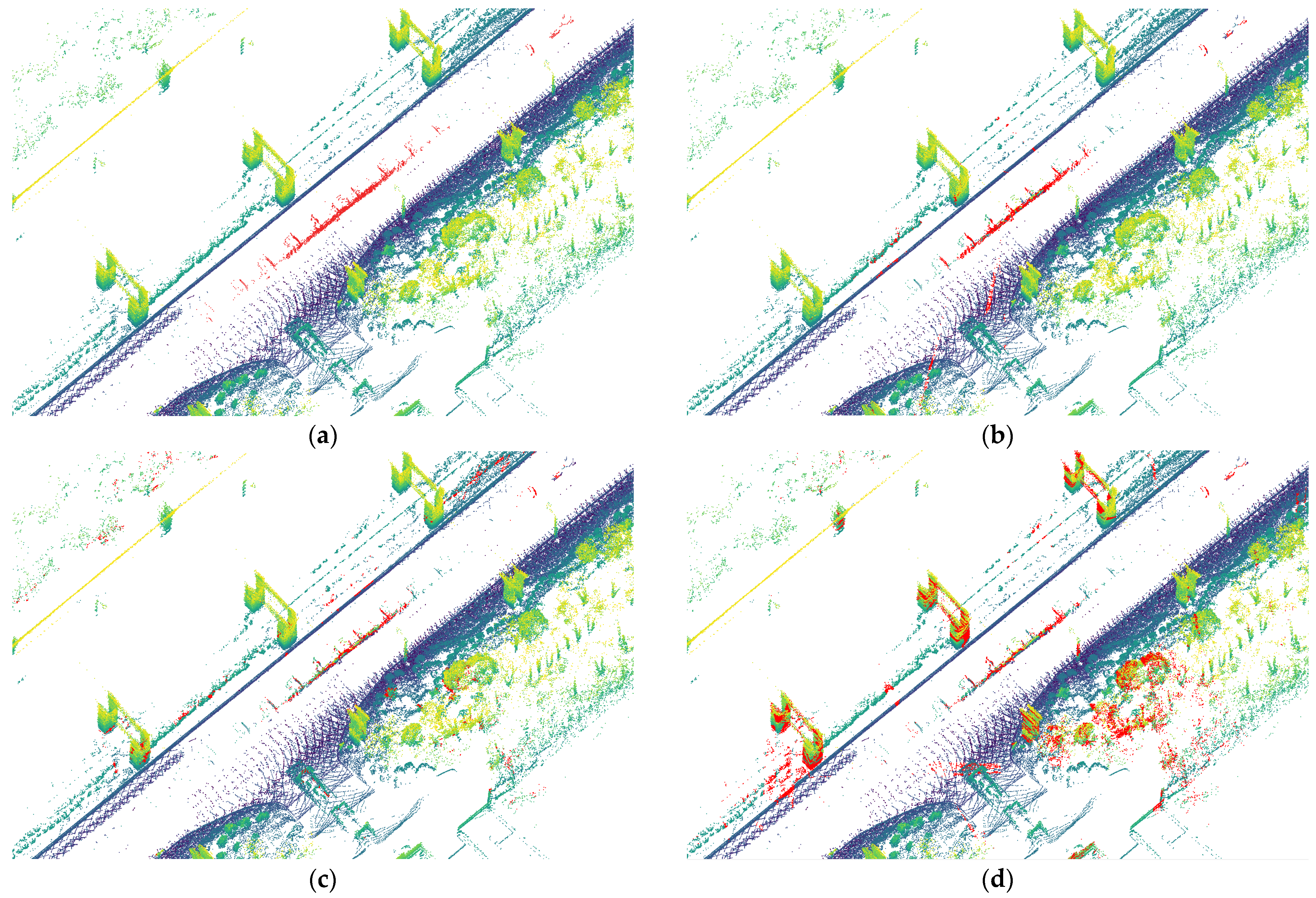
As shown in Figure 4, we exhibit the mapping results based on dataset City1 using SLAM system Lego-LOAM [20]. When translation errors in registration increase, Peopleremover and Removert will mislabel many static background points. By leveraging geometric constraints and the prior pose from IMU measurements, our method can effectively handle such challenging scenarios and provide more reliable results.

5.2. Performance in the Scenarios of LiDAR Registration Failure

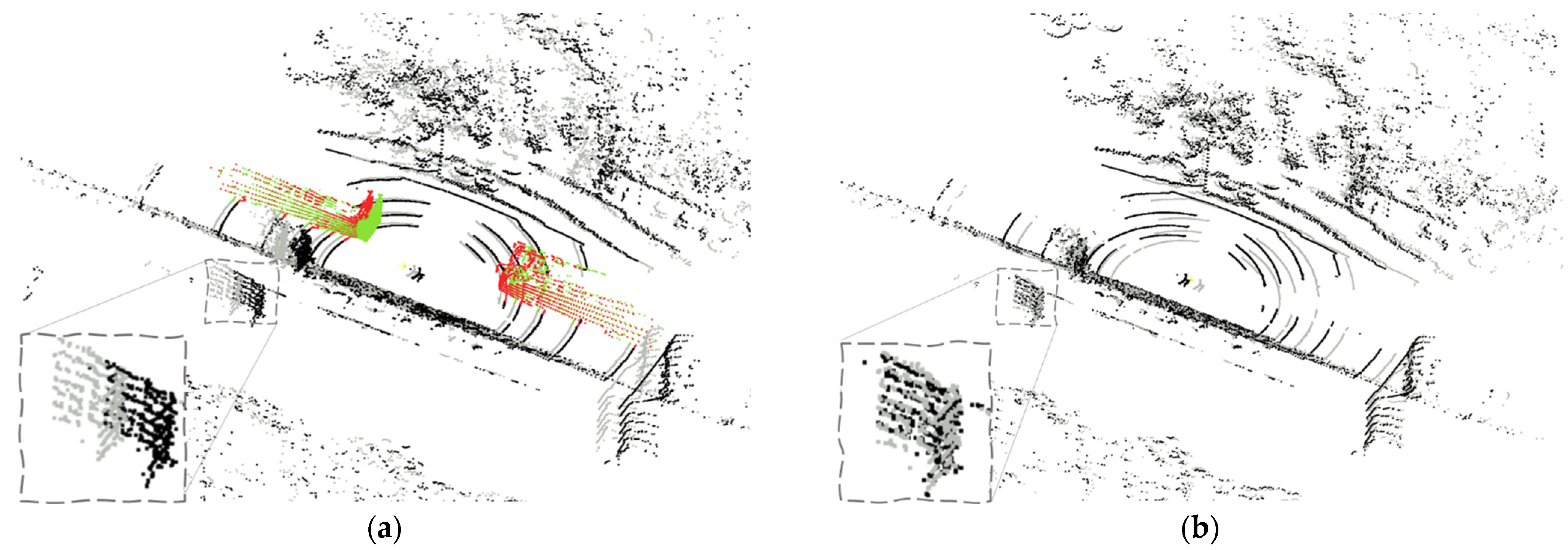
The experiment in this section investigates that our method can be worked in the scenarios of LiDAR registration failure. In datasets City1 and City2, there are some scenarios involving too large and close moving vehicles, which will increase the translation error of registration. In Figure 5a, the occlusion caused by a long vehicle prevents the perfect alignment of two consecutive scans. Notably, existing methods such as Peopleremover and Removert face challenges in accurately identifying moving objects under low-precision registration conditions. However, our method successfully overcomes these challenges. LiDAR registration can be significantly enhanced by leveraging our method for the removal of moving objects, as depicted in Figure 5b.

5.3. Ablation Experiment

In this section, the ablation experiment aims to analyze the performance degradation caused by removing different modules. The evaluation is conducted on dataset City1.

Table 3. Ablation study.

Methods	mIoU (%)
Full pipeline	44.2
(w/o) weight adjustment	38.7
(w/o) ground constraint	42.0
(w/o) region growth	43.6

demonstrates that the full pipeline achieves a performance of up to 44.2% on mIoU. However, removing any of the modules can result in a degradation of performance. Notably, among all the modules, fine estimate with weight adjustment contributes significantly to the overall performance.

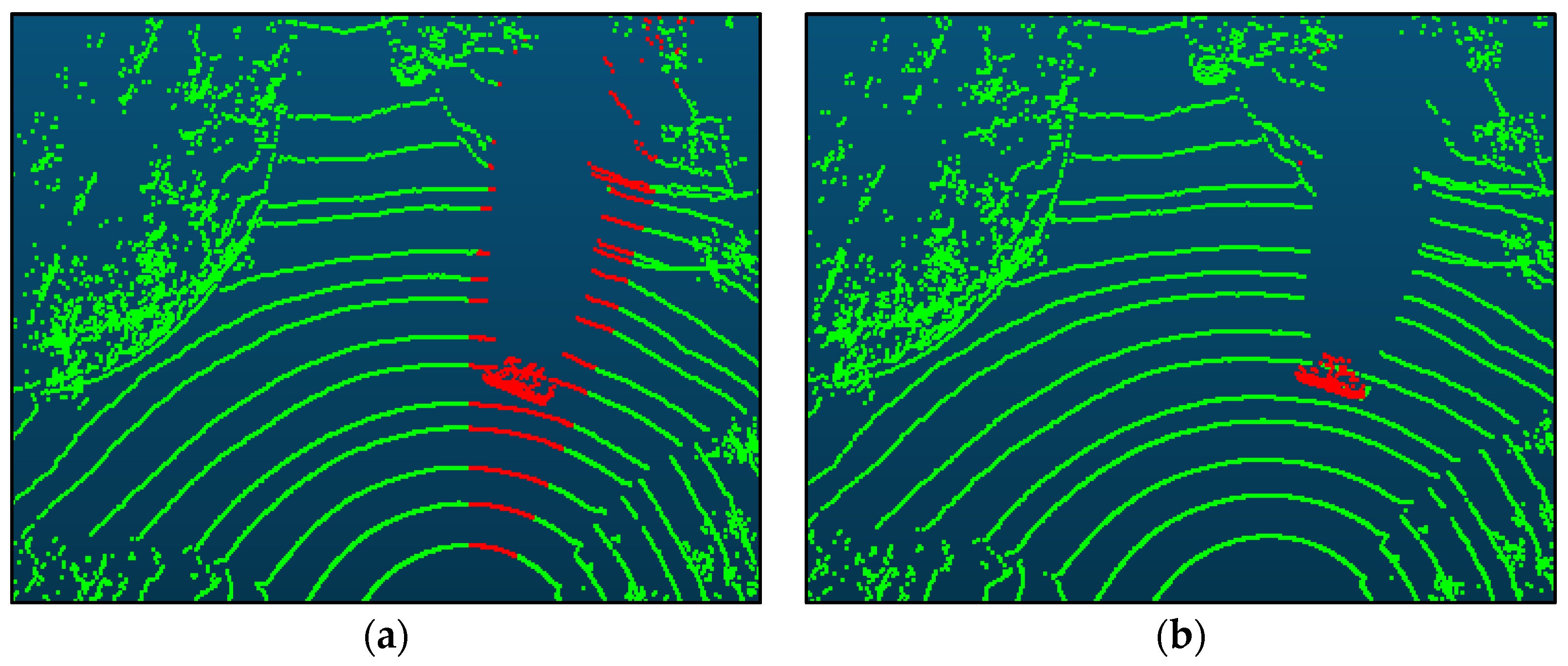
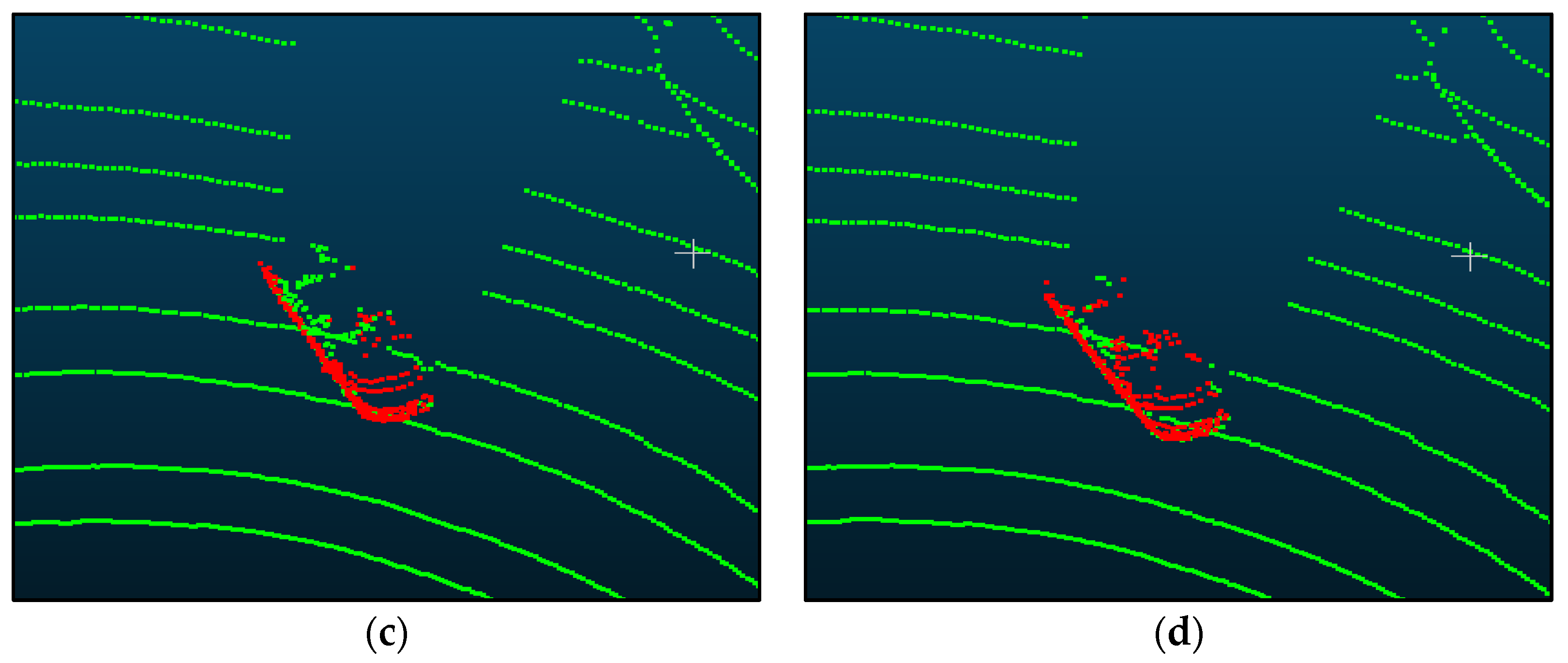
The role of postprocessing is exemplified through visual examples, as depicted in Figure 6. Our investigation revealed that ground points in close proximity to moving targets were susceptible to incorrect labeling, as shown in Figure 6a. To address this issue, we impose a ground constraint on each scan. By incorporating ground detection techniques, we were able to successfully identify and remove the mislabeled ground points, as illustrated in Figure 6b. Furthermore, we utilized regional growth techniques to refine the final detection results, as illustrated in Figure 6c,d. The ablation experiment revealed that regional growth also contributes to improving detection.

5.4. Runtime

In terms of evaluating computational efficiency, all experiments in this paper were conducted on a consistent platform featuring an Intel [email protected] processor and an NVIDIA GeForce GTX1060 graphics card. We calculated the average runtime for each scan using our method and compared it to Removert and Peopleremover. Our method achieves remarkably faster execution times (93 ms) compared to the baseline methods, such as Removert (1810 ms) and Peopleremover (1202 ms), with the exception of the data I/O module.

5.5. Limitations

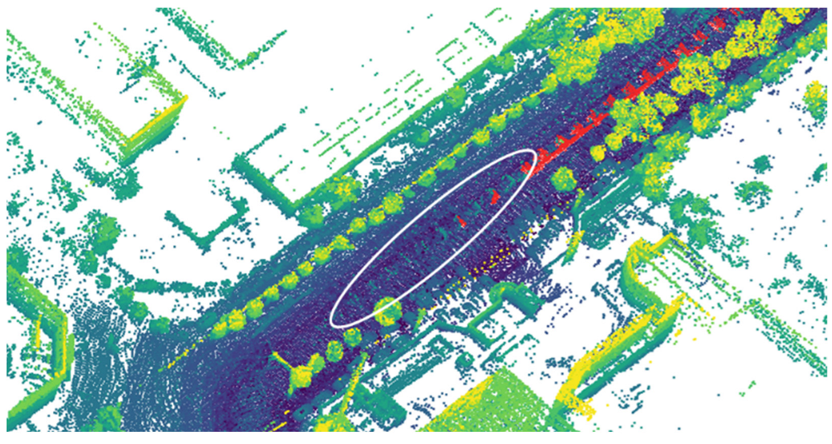
Our method exhibits limitations in effectively detecting small objects at longer distances, often resulting in missed detections. As depicted in Figure 7, when the ego-car is positioned far away from moving objects, the LiDAR captures only a limited number of points. This limited capture may potentially result in the omission of these points during optimization, leading to missed detections. Fortunately, these points belonging to distant moving objects generally have minimal impact on the accuracy of registration. Moreover, we acknowledge that utilizing higher-resolution LiDARs may offer potential improvements to overcome missed detections.

6. Conclusions

In this paper, we propose a novel approach for effectively removing moving objects from 3D laser scans. Unlike existing methods that heavily depend on precise LiDAR registration, our approach accurately estimates dense range flow without the need for registration. By leveraging 3D range-based geometric constraints and integrating IMU measurements, our method significantly enhances the accuracy of dense range flow estimation. Through extensive evaluations on publicly available and self-recorded datasets, our method surpasses the performance of baseline approaches. Notably, in environments where the error of LiDAR registration and odometry increases, our method exhibits superior robustness and accuracy. Furthermore, the absence of annotation requirements allows for seamless integration of our method into SLAM systems with different sensor setups.

This work provides a possibility of removing moving objects before registration, which can improve LiDAR SLAM systems in terms of accumulation errors. However, the limitation of accurately detecting moving objects in small- or longer-distance scenarios, attributed to the sparsity of points, presents an avenue for future improvement.

References

1. Chen, X.; Li, S.; Mersch, B.; Wiesmann, L.; Gall, J.; Behley, J.; Stachniss, C. Moving Object Segmentation in 3D LiDAR Data: A Learning-Based Approach Exploiting Sequential Data. IEEE Robot. Autom. Lett. 2021, 6, 6529–6536. [Google Scholar] [CrossRef]
2. Lim, H.; Hwang, S.; Myung, H. ERASOR: Egocentric Ratio of Pseudo Occupancy-Based Dynamic Object Removal for Static 3D Point Cloud Map Building. IEEE Robot. Autom. Lett. 2021, 6, 2272–2279. [Google Scholar] [CrossRef]
3. Pomerleau, F.; Krusi, P.; Colas, F.; Furgale, P.; Siegwart, R. Long-Term 3D Map Maintenance in Dynamic Environments. In Proceedings of the 2014 IEEE International Conference on Robotics and Automation (ICRA), Hong Kong, China, 31 May–5 June 2014; pp. 3712–3719. [Google Scholar] [CrossRef] [Green Version]
4. Schauer, J.; Nuchter, A. The Peopleremover—Removing Dynamic Objects from 3-D Point Cloud Data by Traversing a Voxel Occupancy Grid. IEEE Robot. Autom. Lett. 2018, 3, 1679–1686. [Google Scholar] [CrossRef]
5. Moosmann, F.; Fraichard, T. Motion Estimation from Range Images in Dynamic Outdoor Scenes. In Proceedings of the 2010 IEEE International Conference on Robotics and Automation, Anchorage, AK, USA, 3–7 May 2010; pp. 142–147. [Google Scholar] [CrossRef] [Green Version]
6. Pagad, S.; Agarwal, D.; Narayanan, S.; Rangan, K.; Kim, H.; Yalla, G. Robust Method for Removing Dynamic Objects from Point Clouds. In Proceedings of the 2020 IEEE International Conference on Robotics and Automation (ICRA), Paris, France, 31 May–31 August 2020; pp. 10765–10771. [Google Scholar] [CrossRef]
7. Fan, T.; Shen, B.; Chen, H.; Zhang, W.; Pan, J. DynamicFilter: An Online Dynamic Objects Removal Framework for Highly Dynamic Environments. In Proceedings of the 2022 International Conference on Robotics and Automation (ICRA), Philadelphia, PA, USA, 23–27 May 2022. [Google Scholar]
8. Fu, H.; Xue, H.; Xie, G. MapCleaner: Efficiently Removing Moving Objects from Point Cloud Maps in Autonomous Driving Scenarios. Remote Sens. 2022, 14, 4496. [Google Scholar] [CrossRef]
9. Yoon, D.; Tang, T.; Barfoot, T. Mapless Online Detection of Dynamic Objects in 3D Lidar. In Proceedings of the 2019 16th Conference on Computer and Robot Vision (CRV), Kingston, QC, Canada, 29–31 May 2019; pp. 113–120. [Google Scholar] [CrossRef] [Green Version]
10. Kim, G.; Kim, A. Remove, Then Revert: Static Point Cloud Map Construction Using Multiresolution Range Images. In Proceedings of the 2020 IEEE/RSJ International Conference on Intelligent Robots and Systems (IROS), Las Vegas, NV, USA, 25–29 October 2020; pp. 10758–10765. [Google Scholar] [CrossRef]
11. Kim, J.; Woo, J.; Im, S. RVMOS: Range-View Moving Object Segmentation Leveraged by Semantic and Motion Features. IEEE Robot. Autom. Lett. 2022, 7, 8044–8051. [Google Scholar] [CrossRef]
12. Mersch, B.; Chen, X.; Vizzo, I.; Nunes, L.; Behley, J.; Stachniss, C. Receding Moving Object Segmentation in 3D LiDAR Data Using Sparse 4D Convolutions. IEEE Robot. Autom. Lett. 2022, 7, 7503–7510. [Google Scholar] [CrossRef]
13. Pfreundschuh, P.; Hendrikx, H.F.C.; Reijgwart, V.; Dube, R.; Siegwart, R.; Cramariuc, A. Dynamic Object Aware LiDAR SLAM Based on Automatic Generation of Training Data. In Proceedings of the 2021 IEEE International Conference on Robotics and Automation (ICRA), Xi’an, China, 30 May–5 June 2021; pp. 11641–11647. [Google Scholar] [CrossRef]
14. Kreutz, T.; Muhlhauser, M.; Guinea, A.S. Unsupervised 4D LiDAR Moving Object Segmentation in Stationary Settings with Multivariate Occupancy Time Series. In Proceedings of the 2023 IEEE/CVF Winter Conference on Applications of Computer Vision (WACV), Waikoloa, HI, USA, 3–7 January 2023; pp. 1644–1653. [Google Scholar] [CrossRef]
15. Sun, J.; Dai, Y.; Zhang, X.; Xu, J.; Ai, R.; Gu, W.; Chen, X. Efficient Spatial-Temporal Information Fusion for LiDAR-Based 3D Moving Object Segmentation. In Proceedings of the 2022 IEEE/RSJ International Conference on Intelligent Robots and Systems (IROS), Kyoto, Japan, 23–27 October 2022; pp. 11456–11463. [Google Scholar]
16. Guo, Y.; Wang, H.; Hu, Q.; Liu, H.; Liu, L.; Bennamoun, M. Deep Learning for 3D Point Clouds: A Survey. IEEE Trans. Pattern Anal. Mach. Intell. 2021, 43, 4338–4364. [Google Scholar] [CrossRef] [PubMed]
17. Wang, Z.; Li, S.; Howard-Jenkins, H.; Prisacariu, V.; Chen, M. FlowNet3D++: Geometric Losses for Deep Scene Flow Estimation. In Proceedings of the IEEE/CVF Winter Conference on Applications of Computer Vision, Snowmass, CO, USA, 3–8 January 2020; pp. 91–98. [Google Scholar]
18. Liu, X.; Qi, C.R.; Guibas, L.J. FlowNet3D: Learning Scene Flow in 3D Point Clouds. In Proceedings of the 2019 IEEE/CVF Conference on Computer Vision and Pattern Recognition (CVPR), Long Beach, CA, USA, 15–20 June 2019; pp. 529–537. [Google Scholar] [CrossRef] [Green Version]
19. Baur, S.A.; Emmerichs, D.J.; Moosmann, F.; Pinggera, P.; Ommer, B.; Geiger, A. SLIM: Self-Supervised LiDAR Scene Flow and Motion Segmentation. In Proceedings of the 2021 IEEE/CVF International Conference on Computer Vision (ICCV), Montreal, QC, Canada, 10–17 October 2021; pp. 13106–13116. [Google Scholar] [CrossRef]
20. Shan, T.; Englot, B. LeGO-LOAM: Lightweight and Ground-Optimized Lidar Odometry and Mapping on Variable Terrain. In Proceedings of the 2018 IEEE/RSJ International Conference on Intelligent Robots and Systems (IROS), Madrid, Spain, 1–5 October 2018; pp. 4758–4765. [Google Scholar] [CrossRef]
21. Dewan, A.; Caselitz, T.; Tipaldi, G.D.; Burgard, W. Rigid Scene Flow for 3D LiDAR Scans. In Proceedings of the 2016 IEEE/RSJ International Conference on Intelligent Robots and Systems (IROS), Daejeon, Republic of Korea, 9–14 October 2016; pp. 1765–1770. [Google Scholar] [CrossRef]
22. Noorwali, S. Range Flow: New Algorithm Design and Quantitative and Qualitative Analysis. Ph.D. Thesis, The University of Western Ontario, London, ON, Canada, 2020. [Google Scholar]
23. Ahmad, N.; Ghazilla, R.A.R.; Khairi, N.M.; Kasi, V. Reviews on Various Inertial Measurement Unit (IMU) Sensor Applications. IJSPS 2013, 1, 256–262. [Google Scholar] [CrossRef] [Green Version]
24. Sun, R.; Wang, J.; Cheng, Q.; Mao, Y.; Ochieng, W.Y. A New IMU-Aided Multiple GNSS Fault Detection and Exclusion Algorithm for Integrated Navigation in Urban Environments. GPS Solut. 2021, 25, 147. [Google Scholar] [CrossRef]
25. Sukkarieh, S.; Nebot, E.M.; Durrant-Whyte, H.F. A High Integrity IMU/GPS Navigation Loop for Autonomous Land Vehicle Applications. IEEE Trans. Robot. Autom. 1999, 15, 572–578. [Google Scholar] [CrossRef] [Green Version]
26. Bruhn, A.; Weickert, J.; Schnörr, C. Lucas/Kanade Meets Horn/Schunck: Combining Local and Global Optic Flow Methods. Int. J. Comput. Vis. 2005, 61, 211–231. [Google Scholar] [CrossRef] [Green Version]
27. Cui, J.; Zhang, F.; Feng, D.; Li, C.; Li, F.; Tian, Q. An Improved SLAM Based on RK-VIF: Vision and Inertial Information Fusion via Runge-Kutta Method. Def. Technol. 2023, 21, 133–146. [Google Scholar] [CrossRef]
28. Bogoslavskyi, I.; Stachniss, C. Efficient Online Segmentation for Sparse 3D Laser Scans. PFG 2017, 85, 41–52. [Google Scholar] [CrossRef]
29. Velodyne. Velodyne VLP-32C User Manual. Available online: http://www.velodynelidar.com (accessed on 20 May 2023).
30. Spies, H.; Jähne, B.; Barron, J.L. Range Flow Estimation. Comput. Vis. Image Underst. 2002, 85, 209–231. [Google Scholar] [CrossRef]
31. Jaimez, M.; Monroy, J.G.; Gonzalez-Jimenez, J. Planar Odometry from a Radial Laser Scanner. A Range Flow-Based Approach. In Proceedings of the 2016 IEEE International Conference on Robotics and Automation (ICRA), Stockholm, Sweden, 16–21 May 2016; pp. 4479–4485. [Google Scholar] [CrossRef]
32. Behley, J.; Garbade, M.; Milioto, A.; Quenzel, J.; Behnke, S.; Stachniss, C.; Gall, J. SemanticKITTI: A Dataset for Semantic Scene Understanding of LiDAR Sequences. In Proceedings of the IEEE/CVF International Conference on Computer Vision, Seoul, Republic of Korea, 27 October–2 November 2019; pp. 9296–9306. [Google Scholar] [CrossRef] [Green Version]
Figure 1. An example for identifying a moving vehicle using our method. The top and second rows represent range images of the previous and current scans colored by range magnitude. The red pixels in the bottom row stand for the moving vehicle.
Remotesensing 15 03390 g001
Figure 2. Overview of the proposed pipeline.
Remotesensing 15 03390 g002
Figure 3. Visual examples of three datasets. (a) Frame 200 in sequence 01 of the dataset SemanticKITTI. (b) Vehicle platform for capturing datasets City1 and City2. (c) Frame 92 of the dataset City1 ((left) image; (right) point clouds). (d) Frame 110 of the dataset City2 ((left) image; (right) point clouds).
Remotesensing 15 03390 g003
Figure 4. Mapping results on Frame 130–210 of dataset City1, in which moving objects are highlighted in red. (a) ground truth. (b) our method. (c) Removert. (d) Peopleremover.
Remotesensing 15 03390 g004
Figure 5. LiDAR registration can be improved after moving objects removal based on our method. (a) registration before moving objects removal. (b) registration after moving objects removal.
Remotesensing 15 03390 g005
Figure 6. The effect of ground constraint and region growth in the proposed pipeline. (a) w/o ground removal. (b) with ground removal. (c) w/o region growth. (d) with region growth.
Remotesensing 15 03390 g006aRemotesensing 15 03390 g006b
Figure 7. The map from Frame 50–110 in dataset City2, where the white ellipse contains the missed detection car at long distances.
Remotesensing 15 03390 g007