Article

Homography Matrix-Based Local Motion Consistent Matching for Remote Sensing Images

1
Key Laboratory of Opto-Electronic Information Processing, Chinese Academy of Sciences, Shenyang 110016, China
2
Shenyang Institute of Automation, Chinese Academy of Sciences, Shenyang 110016, China
3
Institutes for Robotics and Intelligent Manufacturing, Chinese Academy of Sciences, Shenyang 110169, China
4
University of Chinese Academy of Sciences, Beijing 100049, China
*
Author to whom correspondence should be addressed.
Remote Sens. 2023, 15(13), 3379; https://doi.org/10.3390/rs15133379
Submission received: 12 April 2023 / Revised: 28 June 2023 / Accepted: 29 June 2023 / Published: 2 July 2023
(This article belongs to the Special Issue Machine Vision and Advanced Image Processing in Remote Sensing II)

Abstract

:
Feature matching is a fundamental task in the field of image processing, aimed at ensuring correct correspondence between two sets of features. Putative matches constructed based on the similarity of descriptors always contain a large number of false matches. To eliminate these false matches, we propose a remote sensing image feature matching method called LMC (local motion consistency), where local motion consistency refers to the property that adjacent correct matches have the same motion. The core idea of LMC is to find neighborhoods with correct motion trends and retain matches with the same motion. To achieve this, we design a local geometric constraint using a homography matrix to represent local motion consistency. This constraint has projective invariance and is applicable to various types of transformations. To avoid outliers affecting the search for neighborhoods with correct motion, we introduce a resampling method to construct neighborhoods. Moreover, we design a jump-out mechanism to exit the loop without searching all possible cases, thereby reducing runtime. LMC can process over 1000 putative matches within 100 ms. Experimental evaluations on diverse image datasets, including SUIRD, RS, and DTU, demonstrate that LMC achieves a higher F-score and superior overall matching performance compared to state-of-the-art methods.

1. Introduction

Feature matching is one of the fundamental problems in the field of image processing [1], aiming to establish reliable correspondences between image pairs for various types of transformations. The matching performance of feature matching methods is crucial for many tasks, such as 3D reconstruction [2,3], image registration and fusion [4,5,6], image stitching [7,8], etc. These tasks have high requirements regarding the feature matching methods in terms of robustness, accuracy, and efficiency.
The feature matching problem exhibits a combinatorial property [9]. For example, matching N points from one set to M points in another set produces M N different matching results, resulting in exponential time complexity. To address this problem, a mainstream approach now is to use an indirect feature matching strategy with a two-stage process. In the first stage, feature descriptor methods such as SIFT [10], SURF [11], and ORB [12] are used to create a set of putative matches based on the similarity of local patch descriptors. These methods greatly reduce the time complexity of feature matching problems. However, the ambiguity of local descriptors leads to a significant number of false matches in the set of putative matches. Thus, a geometric constraint is necessary in the second stage to distinguish between correct matches (i.e., inliers) and false matches (i.e., outliers) in the set of putative matches.
The second stage, also known as mismatch removal, is one of the key challenges faced by current indirect feature matching methods. To eliminate false matches, numerous methods have been proposed. In the following, we categorize mismatch removal methods into the following five types and provide a brief review.

1.1. Resampling-Based Methods

Random sample consensus (RANSAC) [13] is a classic resampling method used to estimate a model. The main idea of RANSAC is to randomly select a small subset of data to estimate model parameters, test the remaining data with the estimated model, and distinguish between data that fit the model and data that do not fit the model. RANSAC is typically used in mismatch removal methods to estimate homography matrices. Many improved RANSAC methods have been proposed, such as maximum likelihood estimator sample consensus (MLESAC) [14], progressive sample consensus (PROSAC) [15], marginalizing sample consensus (MAGSAC++) [16], Graph-Cut RANSAC (GC-RANSAC) [17], and others. The basic idea of PROSAC is to gradually increase the number of sampled points according to a certain probability distribution to select more accurate estimated parameters. MAGSAC++ proposes a σ -consensus method that uses the concept of marginalization to avoid the need for manually setting the threshold in RANSAC. GC-RANSAC selects inliers using graph-cutting methods. These resampling-based methods can be understood as globally modeling the transformations between images. However, when the transformations between images are too complex, global modeling may not represent these transformations well.

1.2. Non-Parametric Model-Based Methods

To handle more complex transformations between images, methods based on non-parametric models have been proposed. Representative methods include the identifying correspondence function (ICF) [18], coherent point drift (CPD) [19], and vector field consensus (VFC) [20]. Among them, VFC assumes that the motion vectors of correct matches have motion consistency, and the vector field composed of the motion vectors of correct matches is smooth. VFC defines an energy function based on this and restores the vector field to consistency, selecting the vectors consistent with the vector field as inliers. However, the models defined by these methods are global and may not be suitable for local transformations. Moreover, because no explicit model is established, these methods typically require more computational resources and time.

1.3. Graph Matching-Based Methods

Most of the previous graph matching methods belonged to direct matching rather than removing false matches by designing similarity constraints [21,22,23]. Graph matching methods are formulated as quadratic assignment problems (QAP) [24], which are usually computationally complex and not widely applicable. Recently, graph matching methods have emerged to remove false matches, such as local graph structure consensus (LGSC) [25] and motion-consistency-driven matching (MCDM) [26]. LGSC proposes the use of local graph structure consistency to remove false matches based on the consistency of local geometric information, but it does not have an advantage in runtime. MCDM introduces a priori local motion consistency and proposes using a probabilistic graph model to remove false matches, demonstrating good matching results. Using graph-based methods to remove false matches is a relatively novel and feasible approach.

1.4. Learning-Based Methods

With the rise of deep learning, increasing numbers of learning-based methods have been proposed for removing false matches. Earlier methods include learning a two-class classifier for mismatch removal (LMR) [27] and learning to find good correspondence (LFGC) [28]. Recently, some novel methods have been proposed, such as SuperGlue [29], a graph attention network (GANet) [30], and a context structure representation network (CSRNet) [31]. SuperGlue proposes to generate reliable matches from local features using graph neural networks. GANet builds on SuperGlue with a multi-head graph attention mechanism and a sparse attention map, effectively making the model lightweight and improving its performance. However, GANet is limited by its specific parameter model, and its generality needs to be improved. CSRNet introduces a context-aware attention mechanism and proposes a permutation-invariant structure representation learning module. However, CSRNet ignores information from the source image and cannot meet the real-time requirements of some high-speed tasks due to its own time complexity. Additionally, there are learning-based methods that are directly applied to graph matching, such as GLMNet [32] and GCAN [33]. The use of deep learning-based approaches has shown great potential in research areas, such as mismatch removal and motion model estimation.

1.5. Local Geometric Constraint-Based Methods

Mismatch removal based on local geometric constraints is currently one of the most popular methods. Unlike global models, local geometric constraint-based methods can better handle situations where the scene undergoes local changes and can maintain performance in feature matching tasks with different types of transformations without changing their own model. Local geometric constraint-based methods can typically achieve high accuracy or fast speed when processing with various types of image transformations.
Classical and representative methods include locality preserving matching (LPM) [34] and grid-based motion statistics (GMS) [35]. These two methods are simple and robust, but their constraint abilities still need to be improved. Subsequently, a series of methods have been proposed to enhance their constraint abilities. Local structure consistency constraint (LSCC) [36] introduces the Pearson correlation coefficient to measure the consistency of the structure of feature points’ neighborhoods. Multi-scale locality and rank preservation (mTopKRP) [37] defines rank list distance measurements based on multi-scale neighborhoods to more strictly and generally preserve local topological structure. The multi-neighborhood guided Kendall rank correlation coefficient (mGKRCC) [38] proposes that the neighborhood points of feature points have rank consistency and uses the Kendall correlation coefficient to measure the error in the rank order of neighborhood points. Neighborhood manifold representation consensus (NMRC) [39] proposes iterative filtering of neighborhood construction to obtain more reliable neighborhood points and uses manifold learning to preserve inliers with consistent neighborhood topology. These four methods seek the potential relationships between feature points and their neighboring points through mathematical means, such as correlation, minimizing reconstruction errors, etc.
Apart from these methods, there are other types of methods that predefine a geometric model representing the relationship between feature points and their neighboring points to find inliers. Affine covariant detectors (such as MSER) are used to calculate the reprojection error of two feature point neighborhoods in frame-based probabilistic local verification (IPLV) [40], which proposes a probabilistic model that combines the reprojection error to calculate the probability of feature points being inliers. Local affine preservation (LAP) [41] removes some outliers in the neighborhood points based on the hypothesis that inliers have motion consistency and defines the minimum topological unit (MTU) consisting of the center feature point and its three neighbors. The consistency of neighborhood topology is measured by the ratio of MTUs. IPLV and LAP propose geometric constraints with affine invariance. Considering that affine invariance is a subset of projective invariance, we use homography matrices with projective invariance to design local geometric constraints. Such local geometric constraints have stronger constraint abilities.
For remote sensing images, on the one hand, due to local distortions caused by changes in terrain and imaging viewpoints, spatial relationships become complex [42], and global geometric transformation models cannot represent image transformations well. On the other hand, using complex non-rigid transformation models to represent image transformations would increase the computational complexity of the method. Therefore, it is necessary to design a mismatch removal method that has low time complexity and can handle complex geometric transformations.
In this paper, we propose a remote sensing image feature matching method named LMC (local motion consistency). Based on local motion consistency [34], correct matches have the same motion as their neighboring inliers, while false matches do not. The core idea of LMC is to find neighborhoods with correct motion trends and treat them as local regions, retaining matches that have the same motion as the local region. We conducted experiments on multiple public datasets, and the results show that LMC has linear time complexity and can handle images with complex geometric transformations.
Our contributions can be summarized as follows:
  • We propose a local geometric constraint based on the homography matrix for feature matching in remote sensing images. Compared to other methods based on local geometric constraints, LMC has more strict constraints that aim to utilize the properties of the homography matrix to represent local motion consistency, thereby retaining correct matches. This constraint is projectively invariant and applicable to images with various rigid or non-rigid deformations;
  • We design a jump-out mechanism that can exit the loop without searching through all possible cases, thereby reducing the runtime. LMC can process more than 1000 putative matches within 100 ms;
  • To avoid outliers affecting the search for neighborhoods with correct motion, we introduce a resampling method to construct neighborhoods.
In addition, our proposed method can provide prior knowledge about the homography matrix representing local geometric transformations for subsequent tasks, such as image registration.
The rest of this paper is organized as follows: In Section 2, we provide a detailed description of the proposed LMC method. In Section 3, we compare our method with several state-of-the-art methods on different types of datasets and present qualitative and quantitative experimental evaluations, as well as a robustness analysis. Furthermore, we discuss the impact of different neighborhood construction methods on the performance of LMC. In Section 4, we provide a brief discussion. Finally, in Section 5, we present a brief conclusion.

2. Materials and Methods

In this section, we propose a geometric constraint based on a homography matrix to represent local motion consistency and employ this constraint to remove false matches. We partition the images into many local regions based on the neighborhood of feature points, represent local geometric transformation using a homography matrix, and calculate the reprojection error of feature points to distinguish correct matches from incorrect ones. Additionally, we use RANSAC to build neighborhoods to improve the reliability of constraints and propose a jump-out mechanism to reduce computation time. The flowchart of our proposed method is illustrated in Figure 1.

2.1. Problem Formulation

After obtaining a pair of remote sensing images I x and I y , we use SIFT to obtain a set of putative matching feature point pairs S = { ( x i , y i ) } i = 1 N , where x i and y i R 2 × 1 represent the 2D coordinate vectors of feature points in images I x and I y , respectively, and N represents the total number of feature point pairs.
Due to the inevitable existence of many false matches in the set of putative matches based on feature descriptors, our goal is to remove the false matches (outliers) and retain as many correct matches (inliers) as possible in the given putative matches set S, to obtain the optimal inlier set I * .
We summarized two consensus points from multiple methods [20,25,26,34,35,36,37,38,39,40,41] for removing false matches.
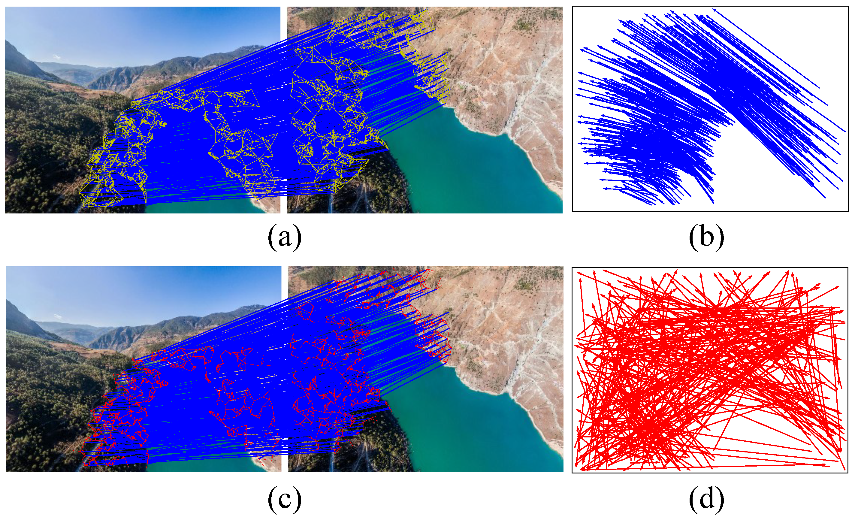
Consensus 1: Motion consistency. The vectors of correct matches (blue vectors in Figure 2b) have similar motions overall, and adjacent vectors have consistent motions, while the vectors of false matches (red vectors in Figure 2d) tend to exhibit random motion across the entire image. We refer to the consistent motion between adjacent vectors of correct matches as local motion consistency.
Consensus 2: Neighborhood topology stability. Real objects are subject to their physical models, which causes the neighborhood topology of feature points to slightly change after geometric transformation, but it is usually stable. The stability of the neighborhood topology of feature points is usually manifested when both the feature point and the points that make up the neighborhood are inliers, as shown in the yellow topology in Figure 2a. However, when there are outliers among the neighborhood points, the neighborhood topology usually lacks stability, as shown in the red topology in Figure 2c.
Therefore, we can design a local geometric constraint that uses the neighborhood to measure the local motion consistency of the matches to determine whether a match is correct. To this end, we formalize the problem of mismatch removal as follows:
I * = arg min I C ( I ; S , λ ) ,
with the cost function C defined as follows:
C ( I ; S , λ ) = i I E r r o r ( x i , y i ) + λ ( N | I | ) ,
where I represents the set of inliers, | I | represents the cardinality of I , and  E r r o r ( x i , y i ) represents the degree of motion consistency between the match ( x i , y i ) and its neighborhood. A larger value of E r r o r ( x i , y i ) indicates greater inconsistency, and hence a higher probability that ( x i , y i ) is a false match. The cost function C consists of two terms: the first penalizes any matches with E r r o r ( x i , y i ) > 0 , while the second is used to retain more inliers. Thus, to obtain the optimal solution of the cost function C, we aim to maximize the number of inliers | I | while minimizing E r r o r ( x i , y i ) as much as possible, with the parameter λ used to balance these two terms. Next, we will introduce how to construct a reliable neighborhood set U and design local geometric constraints to define E r r o r ( x i , y i ) .

2.2. Building Neighborhoods Based on RANSAC

If we search for neighborhood points in the set of putative matches S, the neighborhood points will inevitably be contaminated by outliers. Given that the two aforementioned consensuses are based on the case where both feature points and neighborhood points are inliers, in order to ensure the reliability of the results of the local geometric constraints, we need to remove outliers from the neighborhood as much as possible. To this end, we use RANSAC to construct a reliable set of neighborhood points.
RANSAC (random sample consensus) is a method based on resampling to estimate model parameters. In this paper, RANSAC is used to estimate the homography matrix. The homography matrix can map a point on one plane to a corresponding point on another plane and is used to describe the mapping relationship between planes, including rotation, translation, scaling, and projection. Assuming that ( u , v ) and ( u , v ) are points in the two planes, their mapping relationship can be expressed as
u v 1 = H u v s . 1 = h 11 h 12 h 13 h 21 h 22 h 23 h 31 h 32 1 u v s . 1 ,
where H represents the homography matrix, which can be solved using SVD or Gaussian elimination. Because it has eight parameters, at least four pairs of points are required to compute it.
The steps to estimate the homography matrix using RANSAC are as follows: First, a random sample of corresponding point pairs is selected from the set of matches S. Using these point pairs, a homography matrix is computed. The homography matrix is then used to project the remaining point pairs, and the reprojection error between the projected points and their actual locations is computed. If the error is less than a predefined threshold α , the corresponding point pair is considered an inlier. The process is repeated by resampling until the stopping criteria are met. The homography matrix H RANSAC that can validate the most inliers is selected as the optimal solution, and the validated inliers are regarded as the reliable neighborhood point set U. As a global geometric transformation model, RANSAC constrains the overall motion trend of the neighborhood point set U to be consistent with the planar motion trend represented by H RANSAC , which ensures that U does not contain some randomly distributed outliers. The threshold α controls the strength of the constraint, with smaller α leading to stronger constraints.

2.3. Calculation of Reprojection Error Based on Homography Matrix

The complex non-rigid transformations in remote sensing images cannot be represented by a global geometric transformation model due to factors such as terrain changes, imaging viewpoint changes, and local non-rigid geometric distortion [41]. However, global complex geometric transformations can be approximated by many local simple geometric transformations, which is a common idea in image stitching and matching methods. Considering that the homography matrix is a geometric model that can represent simple geometric transformations (such as affine and projection), we attempt to use the homography matrix to represent local geometric transformations. Therefore, in this section, we introduce the use of a homography matrix to calculate the reprojection error to measure the local motion consistency between feature points and the minimum homography unit (MHU).
We search for the K nearest neighboring points of each feature point x i in the reliable neighborhood point set U under the Euclidean distance and construct the neighborhood N x i K . Similarly, we construct the neighborhood N y i K for feature point y . Because the neighboring points are obtained by searching under the Euclidean distance, the points in N x i K and N y i K may not correspond one-to-one in the putative set S. We need to extract the matched points from N x i K and N y i K , generate a set of matched neighborhood point pairs R i , and use the points in R i to compute the homography matrix. The expression for R i is
R i = { ( x j , y j ) | x j N x i K , y j N y i K } .
The homography matrix H is a 3 × 3 matrix with 8 degrees of freedom; thus, at least 4 pairs of feature points are required for its estimation. We need to select four distinct pairs of feature points from R i to construct the minimum homography unit (MHU) for homography matrix computation, as follows:
M i = C k i 4 = k i ! 4 ! × ( k i 4 ) ! ,
where k i represents the cardinality of R i , i.e.,  k i = | R i | . M i represents the number of possible combinations of neighborhood points in R i used to calculate the homography matrix. All neighborhood points in R i can be found by their indices in the putative set S, and we store these indices in the index matrix q R M i × 4 . Thus, q m n ( m M i , n 4 ) denotes the index of the n-th neighborhood point in the m-th combination in S.
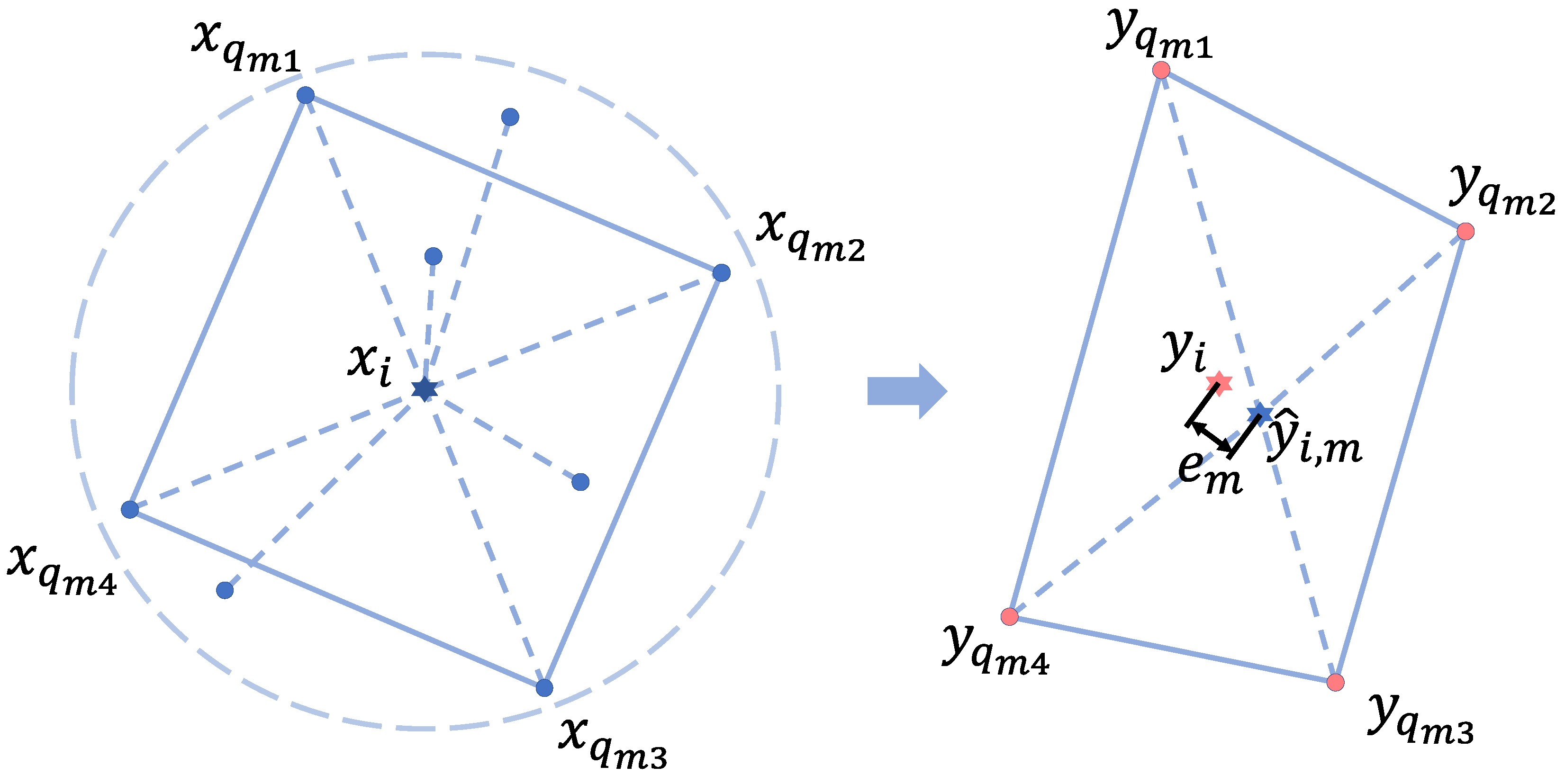
In Figure 3, { ( x q m 1 , y q m 1 ) , ( x q m 2 , y q m 2 ) , ( x q m 3 , y q m 3 ) , ( x q m 4 , y q m 4 ) } represents the m-th MHU. x q m 1 , x q m 2 , x q m 3 , and  x q m 4 denote the neighborhood points of x i in the m-th combination, and the quadrilateral formed by these four points represents the neighborhood of x i . A dashed line connects these four points and x i to create a neighborhood topology. Unlabeled points represent other neighborhood points of x i . y q m 1 , y q m 2 , y q m 3 , and  y q m 4 denote the matching points of x i ’s neighborhood points in y i ’s neighborhood, where y i is the putative matching point of x i , y ^ i , m is the point where x i is projected onto the image I y according to the geometric transformation of the neighborhood, and  e m represents the reprojection error.
First, it is necessary to compute the homography matrix that represents the geometric transformation of the neighborhood. Thus, we have
y q m n 1 = H i , m x q m n 1 ,
where H i , m represents the homography matrix calculated based on the m-th MHU of match ( x i , y i ) , which can be solved by Gaussian elimination. ( x q m n , 1 ) T and ( y q m n , 1 ) T ( m M i , n 4 ) , respectively, represent the homogeneous 3D coordinates of the n-th neighborhood point in the m-th MHU of x i and y i . Based on H i , m , the projection of x i onto image I y can be calculated as follows:
y ^ i , m 1 = H i , m x i 1 ,
where y ^ i , m represents the mapping of feature point x i to the image I y obtained using the homography matrix H i , m . H i , m represents the motion trend of the MHU. According to local motion consistency, if  ( x i , y i ) is a correct match, the motion trend of ( x i , y i ) should be consistent with that of the MHU, i.e., the distance between y i and y ^ i , m should be small.
Therefore, the Euclidean distance between y i and y ^ i , m is used to measure the motion consistency between ( x i , y i ) and the m-th MHU:
e m ( x i , y i ) = y ^ i , m y i 2 ,
where e m ( x i , y i ) represents the reprojection error calculated by x i and y i using H i , m . A smaller value of e m ( x i , y i ) indicates a higher level of motion consistency between ( x i , y i ) and the m-th MHU, indicating a higher probability of ( x i , y i ) being the correct match.
It should be noted that, in theory, local motion consistency is only valid when the feature point and its neighborhood are all inliers. Therefore, if one e m ( x i , y i ) value is very small, we can infer that ( x i , y i ) is likely to be a correct match. However, the MHU may be contaminated by outliers in its neighborhood, so we cannot directly judge the correctness of ( x i , y i ) if one e m ( x i , y i ) value is very large. To avoid contaminated MHUs affecting the correct calculation of MHUs, we should avoid integrating the results of multiple MHUs. Therefore, we choose to use only the minimum e m ( x i , y i ) to represent the probability that ( x i , y i ) is the correct match.
The local geometric constraints in the cost function (1) can be expressed as
E r r o r ( x i , y i ) = min e m ( x i , y i ) , m = 1 , , M i .

2.4. Jump-Out Mechanism

Because the local geometric constraint function E r r o r ( x i , y i ) needs to calculate the minimum e m ( x i , y i ) value every time to serve as its output, this can result in significant computation time. Therefore, in this section, we design a jump-out mechanism to shorten the processing time while minimizing the impact on method accuracy.
We define a binary variable p R N × 1 to represent the matching relationship, where p i = 1 indicates that ( x i , y i ) is an inlier, and  p i = 0 indicates that ( x i , y i ) is an outlier. By substituting the binary variable p into the cost function, Equation (2) becomes
C ( p ; S , λ ) = i = 1 N p i E r r o r ( x i , y i ) + λ ( N i = 1 N p i ) .
We can rewrite the equation by combining terms that are related to p i as follows:
C ( p ; S , λ ) = i = 1 N p i ( E r r o r ( x i , y i ) λ ) + λ N .
The second term in the equation is a constant. To minimize the cost function, we should retain as many negative terms as possible and eliminate positive terms in the first term. Therefore, we define p i as
p i = 1 , E r r o r ( x i , y i ) λ 0 , E r r o r ( x i , y i ) > λ , i = 1 , , N .
Based on local motion consistency, only an MHU that consists entirely of inliers can be used to assess the match, and its assessment result will be reliable. We refer to this kind of MHU as a reliable MHU. The number of reliable MHUs for a match may range from 0 to M i , depending on the inlier ratio in the neighborhood. When there are more than four inliers in the neighborhood, the number of reliable MHUs will exceed 1 and will be randomly distributed among the M i MHUs. In other words, if a match is correct in this case, there may be multiple reliable MHUs with sufficiently small reprojection errors. Therefore, we set a threshold τ , and if there exists an m such that e m ( x i , y i ) τ , then the mth MHU is reliable, and the match ( x i , y i ) is locally motion consistent with this MHU, indicating that it is a correct match. As a result, we redefine p i as
p i = 1 , if m M i s . t . e m ( x i , y i ) τ 0 , otherwise .
Therefore, the optimal inlier set I * can be represented as
I * = { ( x i , y i ) | p i = 1 , i = 1 , 2 , , N } .
If there exists an m that satisfies the conditions of Equation (13), the method can stop calculating E r r o r ( x i , y i ) and jump out of the current loop early to calculate the next E r r o r ( x i + 1 , y i + 1 ) . It can be seen that, theoretically, the loop can only be prematurely exited when the match is correct. Therefore, as the inlier rate of the putative matching set decreases, the ability of this mechanism to shorten the running time will diminish. When the value of τ is the same as λ , the mechanism can significantly reduce the method’s running time with almost no impact on its accuracy. The feasibility of this mechanism will be demonstrated in the ablation study section.

2.5. Time Complexity

As the method proposed in this paper mainly defines a geometric constraint based on a homography matrix to represent local motion consistency, we have abbreviated the proposed method as LMC and summarize it in Algorithm 1. Given a putative match set S with N point pairs, the time complexity for building a reliable neighborhood set U using RANSAC is O ( i N ) , where i is the number of iterations for RANSAC. Using a K-D tree to search for the K nearest neighbors of each feature point in S has a time complexity close to O ( ( K + N ) log N ) . The time complexity for computing the reprojection error of neighborhood homography is at most O ( M N ) , where M is calculated from Equation (5). The total time complexity for the proposed LMC is at most O ( i N + ( K + N ) log N + M N ) . When the iteration count i and neighborhood size K are strictly controlled, the total time complexity can be simplified to O ( N log N ) , as i, M, and K are constants and are smaller than N. The proposed method has linear time complexity and is therefore suitable for handling real-world tasks.
Algorithm 1 The LMC Algorithm.
Input: 
Putative set S = { ( x i , y i ) } i = 1 N , parameters α , K, τ
Output: 
Inlier set I *
1:
Initialize p = zeros(N)
2:
H RANSAC , U = RANSAC(S, α )
3:
Construct neighborhoods N x i K and N y i K for x i and y i , respectively, based on U.
4:
for i = 1:N do
5:
   Construct R i based on Equation (4).
6:
   Calculate M i based on Equation (5).
7:
   for m = 1: M i  do
8:
     Calculate e m ( x i , y i ) based on Equations (6)–(8).
9:
     if  e m ( x i , y i ) τ  then
10:
         p i = 1
11:
        break
12:
     end if
13:
   end for
14:
end for
15:
Calculate I * based on Equation (14).
It should be noted that there may be one-to-many or many-to-one situations (i.e., x i = x j but y i y j , or x i x j but y i = y j ) in the putative match set S obtained using descriptor-based methods (such as SIFT). Therefore, after computing the reprojection error, we check whether the neighboring points are duplicates. If duplicates are found, the calculation result is discarded.

3. Experimental Results

In this section, we compare our proposed method LMC with several existing advanced methods, including LPM [34], RANSAC [13], mTopKRP [37], NMRC [39], and LSCC [36]. The performance will be evaluated based on the following metrics: recall (R), precision (P), F-score (F), and runtime. The performance metrics are defined as follows:
R = T P T P + F N , P = T P T P + F P , F = 2 × P × R P + R ,
where true positive (TP) represents the inliers that are correctly identified as inliers, false positive (FP) represents the outliers that are incorrectly identified as inliers, false negative (FN) represents the inliers that are incorrectly identified as outliers, and true negative (TN) represents the outliers that are correctly identified as outliers. Recall represents the ratio of correctly identified inliers to the total number of inliers in the sample. Precision represents the ratio of correctly identified inliers to the total number of identified inliers. F-score is the harmonic mean of recall and precision. By observing the F-score, the matching accuracy of the method can be comprehensively evaluated.
For the compared methods, LPM is implemented through its Python source code. RANSAC is implemented through the findHomography() function in Opencv4.6.0. In the findHomography() function, RANSAC dynamically adjusts the size of the minimum subset and adapts the threshold according to the distribution of the current data. Additionally, RANSAC uses a method called Sampson distance to calculate errors, which can handle some noise distributions different from Gaussian. RANSAC is also GPU-accelerated. In fact, RANSAC implemented through the findHomography() function has undergone many improvements and differs significantly from the initial version of RANSAC [13]. However, for better naming consistency in subsequent discussions, we still refer to it as RANSAC. For mTopKRP, we modified its Matlab source code into Python source code and implemented it. The Python source code for NMRC and LSCC was self-reproduced based on the respective papers. The default parameters were used in both methods for the experiments. All experiments were conducted on a desktop computer with an Intel(R) Core(TM) i7-10700 CPU with a clock speed of 2.90GHz, 16GB of RAM, Python 3.9, Opencv 4.6.0, and PyCharm 2021.3.2 (Community Edition).

3.1. Datasets

To evaluate the matching performance of the proposed method, we selected five datasets: SUIRD, HPatches [43], RS [1], DTU [44], and Retina [45]:
  • SUIRD: This dataset contains 60 pairs of low-altitude remote sensing images captured by small drones, covering natural landscapes and urban streets. The geometric transformations between image pairs are caused by viewpoint changes during drone shooting, resulting in a low overlap rate, non-rigid image deformation, and extreme viewpoint changes. The dataset is divided into five groups according to the types of drone viewpoint changes: horizontal rotation (termed Horizontal), vertical rotation (termed Vertical), scaling (termed Scaling), mixed viewpoint changes (termed Mixture), and extreme viewpoint changes (termed Extreme). To better demonstrate the experimental data, we integrated horizontal rotation, vertical rotation, and scaling into simple rotation and scaling (termed R&S) in the dataset;
  • HPatches: This dataset consists of images selected from multiple datasets such as VGG, DTU, and AMOS and is used to evaluate the matching performance of matching methods on common images. The dataset contains 116 sets of image sequences, with 6 images in each set. In each image sequence, the first image is matched with the remaining five images. The images involve variations in rotation, scaling, extreme viewpoint changes, lighting changes, and image compression. The dataset is divided into two groups based on the types of image variations, viewpoint changes (termed HPatches-v), and lighting changes (termed HPatches-i);
  • RS: This dataset consists of four different types of remote sensing image datasets, including SAR, CIAP, UAV, and PAN. The image pairs of SAR were captured by synthetic aperture radar and drones, totaling 18 pairs. The images of CIAP were corrected, but with a small overlap area, totaling 57 pairs. The images of UAV were captured by drones with projection distortion, totaling 35 pairs. The images of PAN were captured at different times, with projection distortion, totaling 18 pairs;
  • DTU: The dataset consists of 131 pairs of images with large viewpoint changes. Due to the presence of large viewpoint changes, there are complex non-rigid deformations between image pairs;
  • Retina: This dataset consists of 70 pairs of multimodal medical retinal images, which exhibit non-rigid deformations between the image pairs.
SUIRD consists of low-altitude remote sensing images, while DTU was captured from a closer distance, resulting in a higher degree of non-rigid transformation compared to SUIRD, despite both datasets having large-angle viewpoint changes. The main matching objects in HPatches are planar images, but there are image pairs with extremely low inlier rates in the dataset. RS is a mixed dataset of remote sensing images that can provide a more comprehensive evaluation of the performance of matching methods for remote sensing images. Retina can further evaluate the matching performance of methods on more complex non-rigid transformation images.
These datasets have an average inlier rate of no more than 60%, which poses a challenge for mismatch removal methods. The ground truth for SUIRD, RS, DTU, and Retina was manually annotated. The ground truth for HPatches was represented by homography matrices, with an error threshold set to 5 pixels, and the putative matches sets were established by SIFT.

3.2. Parameter Settings and Ablation Study

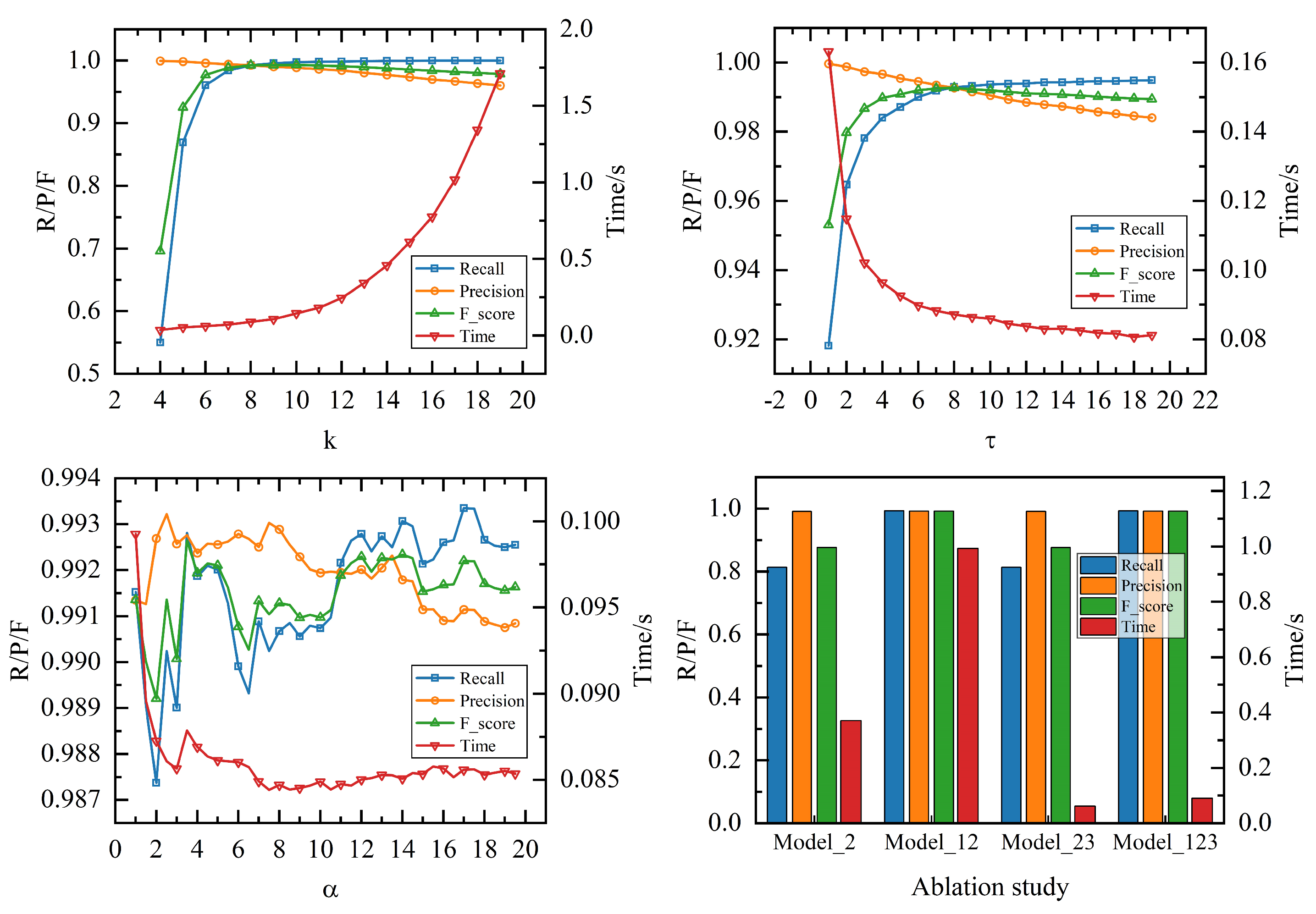
The initial parameters of LMC proposed in this paper include the number of neighbors K, the threshold τ for local motion consistency, and the error threshold α for RANSAC. To test the impact of initial parameters on the performance of LMC, we chose the SUIRD dataset as the test set. Figure 4 shows the curves of the recall (R), precision (P), F-score Fscore(F), and runtime of LMC as the initial parameters change.
Theoretically, the parameter K should not be too large or too small. Based on the motion consistency, inliers typically only have motion consistency with their neighboring inliers, while for farther inliers, they only have similar motion trends. If the K value is too large, it means that the neighborhood of the feature points is large, which reduces the reliability of judging local motion consistency, and the calculation time increases significantly due to the increase in neighboring points. Similarly, if the K value is too small, there may not be enough inliers in the neighborhood to construct the correct MHU, leading to a reduction in the reliability of judging local motion consistency.
As for the τ value, it should be noted that the LMC matching accuracy indicators recall, precision, and F-score only vary in the second decimal place, which indicates that the influence of the τ value on LMC matching accuracy is slight and can distinguish most inliers from outliers. One of the reasons for the change in accuracy indicators is that there are a few outlier positions that are very close to the actual corresponding positions of feature points, which makes LMC unable to distinguish these outliers well within a certain error threshold. Not all such outliers can be distinguished, which depends on the randomness of the outliers and the type of geometric transformation of the neighborhood. Therefore, blindly reducing the τ value will remove some inliers while removing these outliers, and it will also calculate more permutations and combinations, consuming more time.
As for the value of α , it should be noted that LMC performance indicators only change in the third decimal place, so although the curve seems to fluctuate greatly, the impact of α on LMC performance is very slight. The fluctuation in the indicators occurs because RANSAC is a resampling method with certain randomness, and the change in the neighborhood point set has a slight impact on LMC performance. The change in runtime is because the value of α will change the runtime of RANSAC and then change the overall runtime of LMC.
As seen from the above analysis, parameters K and α are usually fixed and only the value of τ is adjusted to balance recall, precision, and runtime. In order to demonstrate the best performance of LMC in the dataset, we set the initial parameter values to K = 8 , τ = 8 , and α = 3.4 .
We divided LMC into three modules: building a reliable neighborhood set using RANSAC, computing the reprojection error using a homography matrix, and using a jump-out mechanism to shorten the runtime. To confirm the effectiveness of these modules, we designed four versions of LMC (Model_2, Model_12, Model_23, and Model_123) for the ablation experiments. The results of these experiments are shown in Figure 4.
The meaning of each version of LMC is as follows:
  • Model_2: Neither RANSAC nor a jump-out mechanism were used.
  • Model_12: Used RANSAC but did not use a jump-out mechanism.
  • Model_23: Used a jump-out mechanism but did not use RANSAC.
  • Model_123: Both RANSAC and a jump-out mechanism were used.
In this experiment, we set λ = τ . From the ablation study in Figure 4, it can be seen that constructing a reliable neighborhood set can effectively improve the matching accuracy of LMC, while the jump-out mechanism can effectively reduce the runtime of LMC.

3.3. Qualitative Analysis

To intuitively understand the matching performance of LMC, we selected 12 representative image pairs from the SUIRD, HPatches, RS, DTU, and Retina datasets to show the matching results, as shown in Figure 5.
It can be seen that LMC can remove most of the false matches for various types of image transformations. The matching results shown in Figure 5 are satisfactory, but there are still a small number of false matches due to four reasons, which we analyze as follows: Firstly, as mentioned earlier, the position of outliers may be very close to the actual corresponding position of the feature points, making it difficult for LMC to distinguish between them. Secondly, the distance between a feature point and the quadrilateral formed by its neighboring points may be so far that, strictly speaking, the quadrilateral cannot be considered as the neighborhood of the feature point, leading to LMC misjudgment. Thirdly, there may be cases where a feature point is an outlier and there are outliers in its neighborhood, but the feature point has a small reprojection error calculated based on these neighborhood points, which is a rare event caused by the randomness of the outliers. Fourthly, a feature point may be very close to or even coincide with a certain neighboring point, making the reprojection error very small and causing LMC misjudgment. These cases may occur in combination. Nevertheless, the LMC proposed by us shows excellent matching results in the SUIRD, HPatches, RS, DTU, and Retina datasets, and the experimental results show that LMC can handle various types of image feature matching.

3.4. Quantitative Analysis

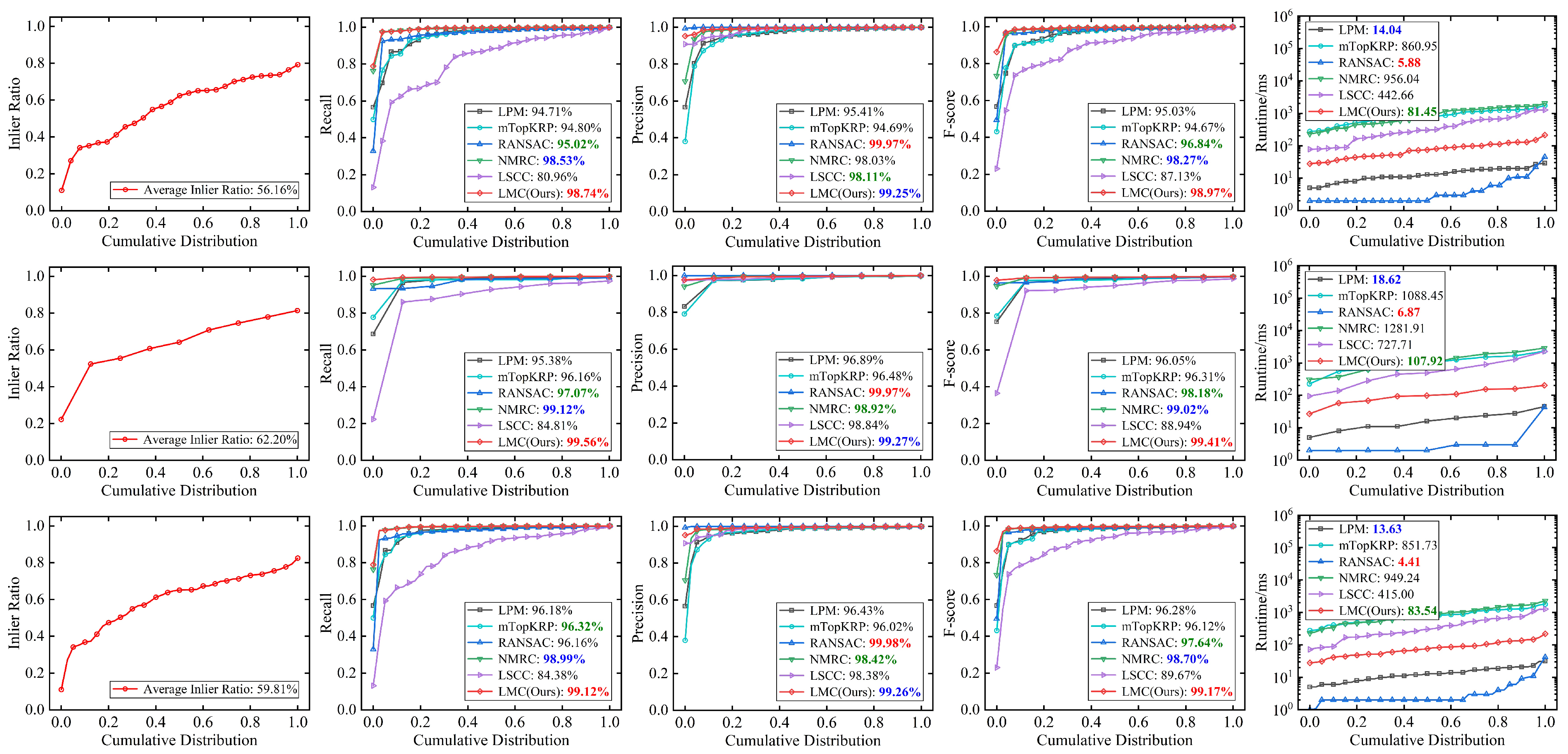
To evaluate the matching performance of the LMC method, we divided the SUIRD dataset into three subsets, Extreme, Mixture, and R&S, and compared it quantitatively with five advanced feature matching methods (LPM [34], RANSAC [13], mTopKRP [37], NMRC [39], and LSCC [36]). We compared these six methods in terms of four performance metrics (recall, precision, F-score, and runtime), as shown in Table 1 and Figure 6.
From Table 1 and Figure 6, it can be seen that the recall and F-score of the LMC method rank first among all six methods on all three datasets, while its precision ranks second, being slightly lower than that of RANSAC. The running time of LMC ranks third. Overall, LMC outperforms the other five advanced methods in terms of matching performance. RANSAC ranks first in precision and runtime, indicating that RANSAC can maximize the inlier ratio of the output results on the SUIRD dataset. However, RANSAC is based on a global geometric transformation model. Although the non-rigid transformations in the SUIRD images are small, there may still be some inliers that do not conform to the global geometric transformation model. Therefore, while ensuring precision, RANSAC always misses some inliers, leading to its third ranking in recall.
LSCC, LPM, mTopKRP, NMRC, and LMC are all based on local geometric constraints. LSCC’s precision ranks fourth, while its recall is the lowest, indicating that Pearson correlation-based methods cannot effectively capture the correlation between neighboring and feature points. LPM’s overall performance is lower than RANSAC’s because LPM is better suited for handling non-rigid transformation scenarios, but the local distortion in the SUIRD dataset is not significant, and LPM did not showcase its advantages. The matching accuracy of mTopKRP and LPM is similar, indicating that their constraint abilities are similar, but LPM’s runtime is significantly lower than mTopKRP. NMRC’s neighborhood manifold-based approach better captures the relationship between neighboring and feature points than LSCC and mTopKRP, with a constraint ability closest to LMC but still slightly lower. We believe that local geometric constraints based on homography matrices have stricter constraint abilities due to their projective invariance. Overall, the LMC method effectively balances recall and precision and has an acceptable runtime, demonstrating superior performance over the other five advanced methods in three different viewpoint change types of datasets.

3.5. Robustness Analysis

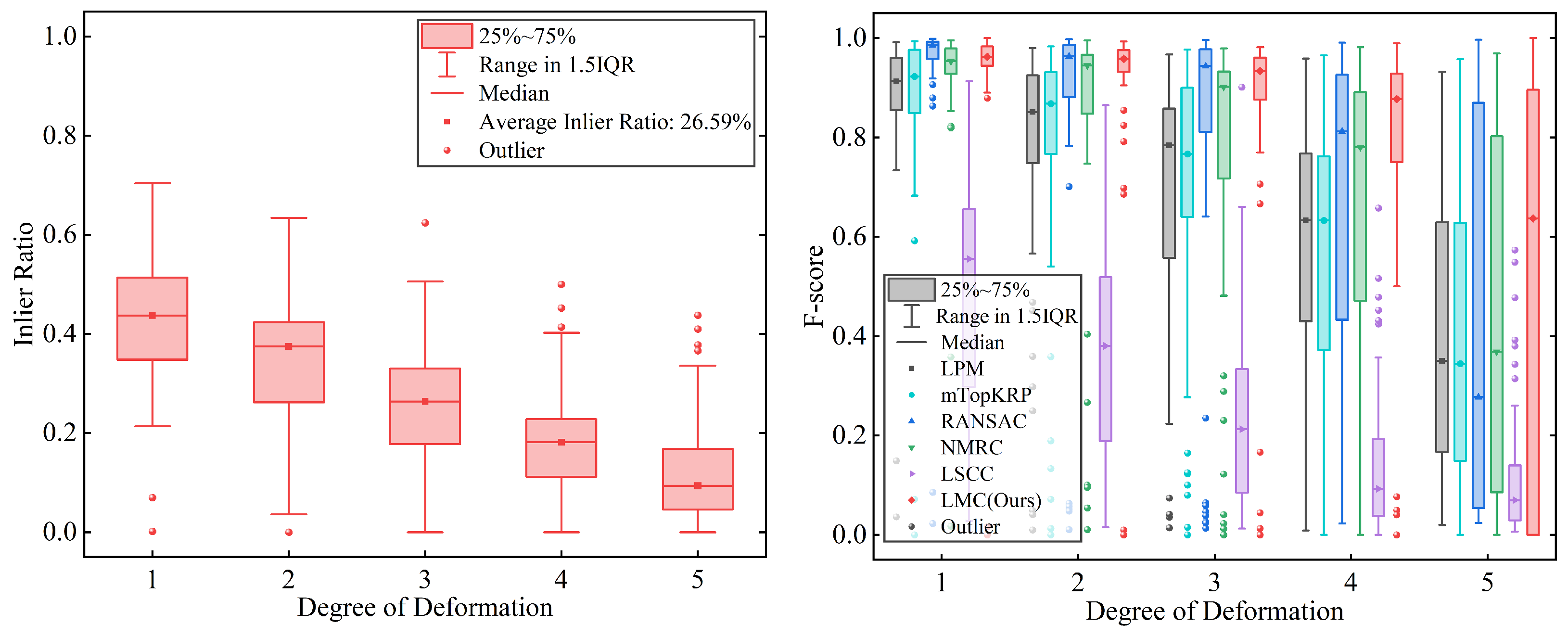
To investigate the matching performance of LMC in image pairs with different inlier ratios, we processed each sequence of image pairs in the HPatches-i dataset and compared the matching performance of LMC with five other state-of-the-art methods. We sorted each group of image pairs by deformation level, as shown in Figure 7. We matched the first image in each row with the remaining five images, resulting in five sets of image pairs. The degree of deformation gradually increases from left to right, and the inlier ratio in the putative sets decreases. We divided each column of image pairs into a group, resulting in five groups. Figure 8 presents a box plot of the inlier ratio and F-score of these five groups and the six methods.
The reason for the appearance of outliers with inlier ratios and F-scores close to 0 in the figure is that there are a few image sequences in HPatches in which the inlier ratio of all image pairs is close to 0, resulting in a sharp drop in method performance and becoming an outlier. As shown in Figure 8, as the inlier ratio decreases, the matching performance of all methods decreases. However, compared with the other five methods, the performance of LMC declines more slowly. Therefore, the stability of LMC with respect to changes in the inlier ratio is superior to that of the other five methods.

3.6. Impact of Neighborhood Construction Methods on Performance

To investigate the impact of different neighborhood construction methods on the performance of the method, we used RANSAC and LPM to construct the neighborhood separately. To distinguish these two methods, we named them LMC_RANSAC and LMC_LPM, respectively. We compared these two methods with five other advanced methods on different types of datasets, including DTU, Retina, RS, HPatches, and SUIRD. When a method could not process a particular image pair, we set its recall, precision, and F-score to 0 and set the runtime to 1000 ms as a penalty. The experimental results are shown in Table 2 and Figure 9.
Based on Table 2, it can be observed that LMC_LPM achieves the highest recall and F-score on the DTU and Retina datasets, while ranking third in terms of running time, which is acceptable. However, LMC_LPM ranks third in terms of precision. RANSAC performs best in precision as it retains global matches with the most consistent motion trends, ensuring that the retained matches are inliers to a greater extent. However, due to varying degrees of non-rigid deformations in the DTU, Retina, and RS datasets, there are inliers in the matches that deviate from the global motion trends. RANSAC fails to preserve these inliers, resulting in a significant decrease in recall compared to precision on these three datasets. Benefiting from the use of RANSAC as the neighborhood construction method, LMC_RANSAC achieves the second highest precision across all five datasets. For the RS dataset, LMC_LPM ranks second in F-score, while recall and precision rank third. Nevertheless, even when LMC_LPM’s F-score is only 0.01% lower than that of NMRC, its running time is only 65% of NMRC’s. On the HPatches dataset, LMC_RANSAC ranks first in F-score and second in recall and precision. However, due to the low inlier rate in the HPatches dataset, all seven methods experience varying degrees of performance degradation. Examining the data in the fourth row of Figure 9, despite having the most image pairs that LMC_RANSAC cannot handle, it still demonstrates better matching performance for the pairs it can handle. Additionally, the average running time of LMC_RANSAC and LMC_LPM increases due to the penalty term, but for the image pairs that can be processed, their running time remains around 100 ms. On the SUIRD dataset, LMC_RANSAC achieves the highest F-score and recall, while ranking second in precision and third in running time. In summary, within an acceptable range of running time, LMC_LPM demonstrates the best overall matching performance on the DTU, Retina, and RS datasets, while LMC_RANSAC exhibits the best overall matching performance on the HPatches and SUIRD datasets.
For neighborhood construction methods, LPM is better suited for handling non-rigid transformation images with complex imaging conditions, such as multimodality, noise interference, and image distortion (such as a wide angle). RANSAC is more suitable for handling relatively simple cases. However, by observing Figure 9, when penalty terms appear in the data of LMC_RANSAC and LMC_LPM, the recall and precision of their neighborhood construction methods always have very low values. Compared with other methods, LMC has stricter requirements for the neighborhood’s inlier rate and the number of putative matches. If the neighborhood’s inlier rate is insufficient, it will cause LMC’s runtime to increase and even reduce the reliability of local geometric constraints in estimating local motion consistency. If the number of putative matches is insufficient, it will cause the neighborhood to be too large, thereby reducing the accuracy of the method.
In general, the experimental data indicate that LMC_LPM is suitable for handling non-rigid transformation images with complex imaging situations and unknown types of image changes. LMC_RANSAC, on the other hand, is suitable for handling relatively simple image transformations. Both algorithms have demonstrated superior matching performance in their respective applicable datasets compared to the current five advanced methods.

4. Discussion

In Section 3.3, we visualized the feature matching performance of LMC in multiple datasets and discussed the reasons for the errors in LMC based on the visualization results, providing ideas for improving LMC. In Section 3.4, we conducted experiments on multiple datasets with various viewpoints, comparing LMC with five other advanced methods and providing a brief analysis of each method. In Section 3.5, we conducted a robustness analysis, which shows that LMC has better robustness to changes in the inlier ratio than other methods but still fails when the inlier ratio is too low. In Section 3.6, we discussed the impact of neighborhood construction methods on LMC’s matching performance. The experimental results show that LMC_LPM and LMC_RANSAC had the best comprehensive matching performance on their respective applicable geometric transformation datasets, with an average runtime of less than 100 ms.
Compared to other methods based on local geometric constraints, LMC uses more strict geometric constraints, which enables it to handle cases with more complex geometric transformations. Therefore, LMC has a wider range of applicability than methods such as RANSAC. In addition to its good feature matching performance in the field of remote sensing images, our proposed method also shows promising potential in other image processing fields, such as feature matching in multimodal medical images.
However, LMC also has strict requirements for the inlier ratio of the neighborhood. If the feature points are too sparse, it may lead to abnormal neighborhood construction, which may in turn reduce the matching performance of LMC. In addition, the runtime of LMC increases as the inlier ratio of the neighborhood decreases. This is because the jump-out mechanism of LMC assumes that there may exist multiple reliable MHUs in the neighborhood. When the inlier ratio of the neighborhood is too low, the number of reliable MHUs in the neighborhood will also decrease, which may degrade or even invalidate the performance of the jump-out mechanism.
Overall, LMC has two limitations. Firstly, LMC heavily relies on the initialization of neighborhoods, making it unable to handle images with very sparse features, such as water surfaces, skies, and white walls. Secondly, LMC is based on the assumption that local regions can be approximated as planes. When the geometric transformations in the image become excessively complex, leading to local regions with intricate non-rigid geometric transformations, LMC’s performance is affected. Considering these limitations, we propose two directions for improvement. To address the first limitation, we can explore designing new feature point detection methods that can detect more features in sparse images. Additionally, we can work on designing faster and more versatile neighborhood construction methods to ensure robust neighborhood initialization. Regarding the second limitation, for more complex local geometric transformations, we can consider using models capable of representing more intricate geometric transformations to design local geometric constraints.

5. Conclusions

This paper proposes a new method for removing mismatches in the feature matching of remote sensing images, called local motion consistency (LMC). LMC is based on the property that adjacent correct matches have the same motion and uses homography matrices to represent neighborhood geometric transformations. This method measures the local motion consistency of matches by calculating the reprojection error of feature points, which allows for the identification and removal of false matches. We propose a jump-out mechanism to significantly reduce the runtime. The experimental results demonstrate that this mechanism can maintain the runtime within 100 ms. Additionally, we utilize RANSAC and LPM for neighborhood construction, dividing the proposed method into LMC_RANSAC and LMC_LPM. The experimental data reveal that LMC_RANSAC and LMC_LPM achieve higher F-scores than other methods on their respective applicable datasets. This indicates that these two methods excel in balancing recall and precision, showcasing superior comprehensive matching performance compared to state-of-the-art approaches.
It should be noted that LMC heavily relies on the initialization of the neighborhood. When putative matches are very sparse or the inlier ratio of the neighborhood is very low, the measure of local motion consistency used by LMC can become unreliable. Fortunately, the neighborhood construction methods that are currently used are generally applicable to most cases, but it is possible to explore the design of faster and more versatile neighborhood construction methods. Additionally, it is worth trying to use geometric transformation models that can represent more complex transformations to represent local motion consistency.

Author Contributions

Conceptualization, J.L. and A.L.; methodology, J.L. and A.L.; software, J.L., A.L. and E.Z.; validation, E.Z. and M.P.; writing—original draft preparation, J.L.; writing—review and editing, J.L., M.P. and D.Z.; supervision, D.Z. All authors have read and agreed to the published version of the manuscript.

Funding

This research was supported by the National Natural Science Foundation of China (62173320).

Data Availability Statement

The dataset SUIRD is available at https://github.com/yyangynu/SUIRD, accessed on 19 March 2023. The dataset HPatches is available at https://github.com/hpatches/hpatches-dataset, accessed on 19 March 2023. The datasets RS, DTU, and Retina can be obtained at https://github.com/StaRainJ/Image_matching_Datasets, accessed on 19 March 2023. The code of our method can be downloaded at https://github.com/Ljy0109/LMC, accessed on 21 March 2023.

Conflicts of Interest

The authors declare no conflict of interest.

References

  1. Ma, J.; Jiang, X.; Fan, A.; Jiang, J.; Yan, J. Image matching from handcrafted to deep features: A survey. Int. J. Comput. Vis. 2021, 129, 23–79. [Google Scholar] [CrossRef]
  2. Li, X.; Luo, X.; Wu, Y.; Li, Z.; Xu, W. Research on stereo matching for satellite generalized image pair based on improved SURF and RFM. In Proceedings of the IGARSS 2020—2020 IEEE International Geoscience and Remote Sensing Symposium, Waikoloa, HI, USA, 26 September–2 October 2020; pp. 2739–2742. [Google Scholar]
  3. Jiang, S.; Jiang, W.; Wang, L. Unmanned aerial vehicle-based photogrammetric 3d mapping: A survey of techniques, applications, and challenges. IEEE Geosci. Remote Sens. Mag. 2021, 10, 135–171. [Google Scholar] [CrossRef]
  4. Xiao, G.; Luo, H.; Zeng, K.; Wei, L.; Ma, J. Robust feature matching for remote sensing image registration via guided hyperplane fitting. IEEE Trans. Geosci. Remote Sens. 2020, 60, 1–14. [Google Scholar] [CrossRef]
  5. Quan, D.; Wang, S.; Gu, Y.; Lei, R.; Yang, B.; Wei, S.; Hou, B.; Jiao, L. Deep feature correlation learning for multi-modal remote sensing image registration. IEEE Trans. Geosci. Remote Sens. 2022, 60, 1–16. [Google Scholar] [CrossRef]
  6. Ma, J.; Tang, L.; Fan, F.; Huang, J.; Mei, X.; Ma, Y. SwinFusion: Cross-domain long-range learning for general image fusion via swin transformer. IEEE/CAA J. Autom. Sin. 2022, 9, 1200–1217. [Google Scholar] [CrossRef]
  7. Lin, C.C.; Pankanti, S.U.; Natesan Ramamurthy, K.; Aravkin, A.Y. Adaptive as-natural-as-possible image stitching. In Proceedings of the IEEE Conference on Computer Vision and Pattern Recognition, Boston, MA, USA, 7–12 June 2015; pp. 1155–1163. [Google Scholar]
  8. Wei, C.; Xia, H.; Qiao, Y. Fast unmanned aerial vehicle image matching combining geometric information and feature similarity. IEEE Geosci. Remote Sens. Lett. 2020, 18, 1731–1735. [Google Scholar] [CrossRef]
  9. Wang, C.; Wang, L.; Liu, L. Progressive mode-seeking on graphs for sparse feature matching. In Computer Vision—ECCV 2014, Proceedings of the 13th European Conference, Zurich, Switzerland, 6–12 September 2014; Proceedings, Part II 13; Springer: Berlin/Heidelberg, Germany, 2014; pp. 788–802. [Google Scholar]
  10. Lowe, D.G. Distinctive image features from scale-invariant keypoints. Int. J. Comput. Vis. 2004, 60, 91–110. [Google Scholar] [CrossRef]
  11. Bay, H.; Ess, A.; Tuytelaars, T.; Van Gool, L. Speeded-up robust features (SURF). Comput. Vis. Image Underst. 2008, 110, 346–359. [Google Scholar] [CrossRef]
  12. Rublee, E.; Rabaud, V.; Konolige, K.; Bradski, G. ORB: An efficient alternative to SIFT or SURF. In Proceedings of the 2011 International Conference on Computer Vision; 2011; pp. 2564–2571. [Google Scholar]
  13. Fischler, M.A.; Bolles, R.C. Random sample consensus: A paradigm for model fitting with applications to image analysis and automated cartography. Commun. ACM 1981, 24, 381–395. [Google Scholar] [CrossRef]
  14. Torr, P.H.; Zisserman, A. MLESAC: A new robust estimator with application to estimating image geometry. Comput. Vis. Image Underst. 2000, 78, 138–156. [Google Scholar] [CrossRef] [Green Version]
  15. Chum, O.; Matas, J. Matching with PROSAC-progressive sample consensus. In Proceedings of the 2005 IEEE Computer Society Conference on Computer Vision and Pattern Recognition (CVPR’05), San Diego, CA, USA, 20–25 June 2005; Volume 1, pp. 220–226. [Google Scholar]
  16. Barath, D.; Noskova, J.; Ivashechkin, M.; Matas, J. MAGSAC++, a fast, reliable and accurate robust estimator. In Proceedings of the IEEE/CVF Conference on Computer Vision and Pattern Recognition (CVPR), Seattle, WA, USA, 13–19 June 2020; pp. 1304–1312. [Google Scholar]
  17. Barath, D.; Matas, J. Graph-cut RANSAC: Local optimization on spatially coherent structures. IEEE Trans. Pattern Anal. Mach. Intell. 2021, 44, 4961–4974. [Google Scholar] [CrossRef] [PubMed]
  18. Li, X.; Hu, Z. Rejecting mismatches by correspondence function. Int. J. Comput. Vis. 2010, 89, 1–17. [Google Scholar] [CrossRef]
  19. Myronenko, A.; Song, X. Point set registration: Coherent point drift. IEEE Trans. Pattern Anal. Mach. Intell. 2010, 32, 2262–2275. [Google Scholar] [CrossRef] [PubMed] [Green Version]
  20. Zhao, J.; Ma, J.; Tian, J.; Ma, J.; Zhang, D. A robust method for vector field learning with application to mismatch removing. In Proceedings of the CVPR 2011, Colorado Springs, CO, USA, 20–25 June 2011; pp. 2977–2984. [Google Scholar]
  21. Liu, H.; Yan, S. Common visual pattern discovery via spatially coherent correspondences. In Proceedings of the 2010 IEEE Computer Society Conference on Computer Vision and Pattern Recognition, San Francisco, CA, USA, 13–18 June 2010; pp. 1609–1616. [Google Scholar]
  22. Zhou, F.; De la Torre, F. Factorized graph matching. In Proceedings of the 2012 IEEE Conference on Computer Vision and Pattern Recognition, Providence, RI, USA, 16–21 June 2012; pp. 127–134. [Google Scholar]
  23. Liu, Z.Y.; Qiao, H. Gnccp—Graduated nonconvexityand concavity procedure. IEEE Trans. Pattern Anal. Mach. Intell. 2013, 36, 1258–1267. [Google Scholar] [CrossRef]
  24. Loiola, E.M.; De Abreu, N.M.M.; Boaventura-Netto, P.O.; Hahn, P.; Querido, T. A survey for the quadratic assignment problem. Eur. J. Oper. Res. 2007, 176, 657–690. [Google Scholar] [CrossRef]
  25. Jiang, X.; Xia, Y.; Zhang, X.P.; Ma, J. Robust image matching via local graph structure consensus. Pattern Recogn. 2022, 126, 108588. [Google Scholar] [CrossRef]
  26. Ma, J.; Fan, A.; Jiang, X.; Xiao, G. Feature matching via motion-consistency driven probabilistic graphical model. Int. J. Comput. Vis. 2022, 130, 2249–2264. [Google Scholar] [CrossRef]
  27. Ma, J.; Jiang, X.; Jiang, J.; Zhao, J.; Guo, X. LMR: Learning a two-class classifier for mismatch removal. IEEE Trans. Image Process. 2019, 28, 4045–4059. [Google Scholar] [CrossRef]
  28. Yi, K.M.; Trulls, E.; Ono, Y.; Lepetit, V.; Salzmann, M.; Fua, P. Learning to find good correspondences. In Proceedings of the IEEE Conference on Computer Vision and Pattern Recognition, Munich, Germany, 8–14 September 2018; pp. 2666–2674. [Google Scholar]
  29. Sarlin, P.E.; DeTone, D.; Malisiewicz, T.; Rabinovich, A. Superglue: Learning feature matching with graph neural networks. In Proceedings of the IEEE/CVF Conference on Computer Vision and Pattern Recognition, Seattle, WA, USA, 13–19 June 2020; pp. 4938–4947. [Google Scholar]
  30. Jiang, X.; Wang, Y.; Fan, A.; Ma, J. Learning for mismatch removal via graph attention networks. ISPRS J. Photogramm. Remote Sens. 2022, 190, 181–195. [Google Scholar] [CrossRef]
  31. Chen, J.; Chen, S.; Chen, X.; Dai, Y.; Yang, Y. Csr-net: Learning adaptive context structure representation for robust feature correspondence. IEEE Trans. Image Process. 2022, 31, 3197–3210. [Google Scholar] [CrossRef]
  32. Jiang, B.; Sun, P.; Luo, B. GLMNet: Graph learning-matching convolutional networks for feature matching. Pattern Recogn. 2022, 121, 108167. [Google Scholar] [CrossRef]
  33. Jiang, Z.; Rahmani, H.; Angelov, P.; Black, S.; Williams, B.M. Graph-context Attention Networks for Size-varied Deep Graph Matching. In Proceedings of the IEEE/CVF Conference on Computer Vision and Pattern Recognition, New Orleans, LA, USA, 18–24 June 2022; pp. 2343–2352. [Google Scholar]
  34. Ma, J.; Zhao, J.; Jiang, J.; Zhou, H.; Guo, X. Locality preserving matching. Int. J. Comput. Vis. 2019, 127, 512–531. [Google Scholar] [CrossRef]
  35. Bian, J.; Lin, W.Y.; Matsushita, Y.; Yeung, S.K.; Nguyen, T.D.; Cheng, M.M. Gms: Grid-based motion statistics for fast, ultra-robust feature correspondence. In Proceedings of the IEEE Conference on Computer Vision and Pattern Recognition, Honolulu, HI, USA, 21–26 July 2017; pp. 4181–4190. [Google Scholar]
  36. Shao, F.; Liu, Z.; An, J. A discriminative point matching algorithm based on local structure consensus constraint. IEEE Geosci. Remote Sens. Lett. 2020, 18, 1366–1370. [Google Scholar] [CrossRef]
  37. Jiang, X.; Jiang, J.; Fan, A.; Wang, Z.; Ma, J. Multiscale locality and rank preservation for robust feature matching of remote sensing images. IEEE Trans. Geosci. Remote Sens. 2019, 57, 6462–6472. [Google Scholar] [CrossRef]
  38. Chen, J.; Yang, M.; Gong, W.; Yu, Y. Multi-neighborhood Guided Kendall Rank Correlation Coefficient for Feature Matching. IEEE Trans. Multimed. 2022. [Google Scholar] [CrossRef]
  39. Ma, J.; Li, Z.; Zhang, K.; Shao, Z.; Xiao, G. Robust feature matching via neighborhood manifold representation consensus. ISPRS J. Photogramm. Remote Sens. 2022, 183, 196–209. [Google Scholar] [CrossRef]
  40. Shen, L.; Xu, Z.; Zhu, J.; Huang, X.; Jin, T. A frame-based probabilistic local verification method for robust correspondence. ISPRS J. Photogramm. Remote Sens. 2022, 192, 232–243. [Google Scholar] [CrossRef]
  41. Ye, X.; Ma, J.; Xiong, H. Local Affine Preservation with Motion Consistency for Feature Matching of Remote Sensing Images. IEEE Trans. Geosci. Remote Sens. 2021, 60, 1–12. [Google Scholar] [CrossRef]
  42. Sedaghat, A.; Mokhtarzade, M.; Ebadi, H. Uniform robust scale-invariant feature matching for optical remote sensing images. IEEE Trans. Geosci. Remote Sens. 2011, 49, 4516–4527. [Google Scholar] [CrossRef]
  43. Balntas, V.; Lenc, K.; Vedaldi, A.; Mikolajczyk, K. HPatches: A benchmark and evaluation of handcrafted and learned local descriptors. In Proceedings of the IEEE Conference on Computer Vision and Pattern Recognition, Honolulu, HI, USA, 21–26 July 2017; pp. 5173–5182. [Google Scholar]
  44. Aanæs, H.; Jensen, R.R.; Vogiatzis, G.; Tola, E.; Dahl, A.B. Large-scale data for multiple-view stereopsis. Int. J. Comput. Vis. 2016, 120, 153–168. [Google Scholar] [CrossRef] [Green Version]
  45. Jiang, X.; Ma, J.; Xiao, G.; Shao, Z.; Guo, X. A review of multimodal image matching: Methods and applications. Inform. Fusion 2021, 73, 22–71. [Google Scholar] [CrossRef]
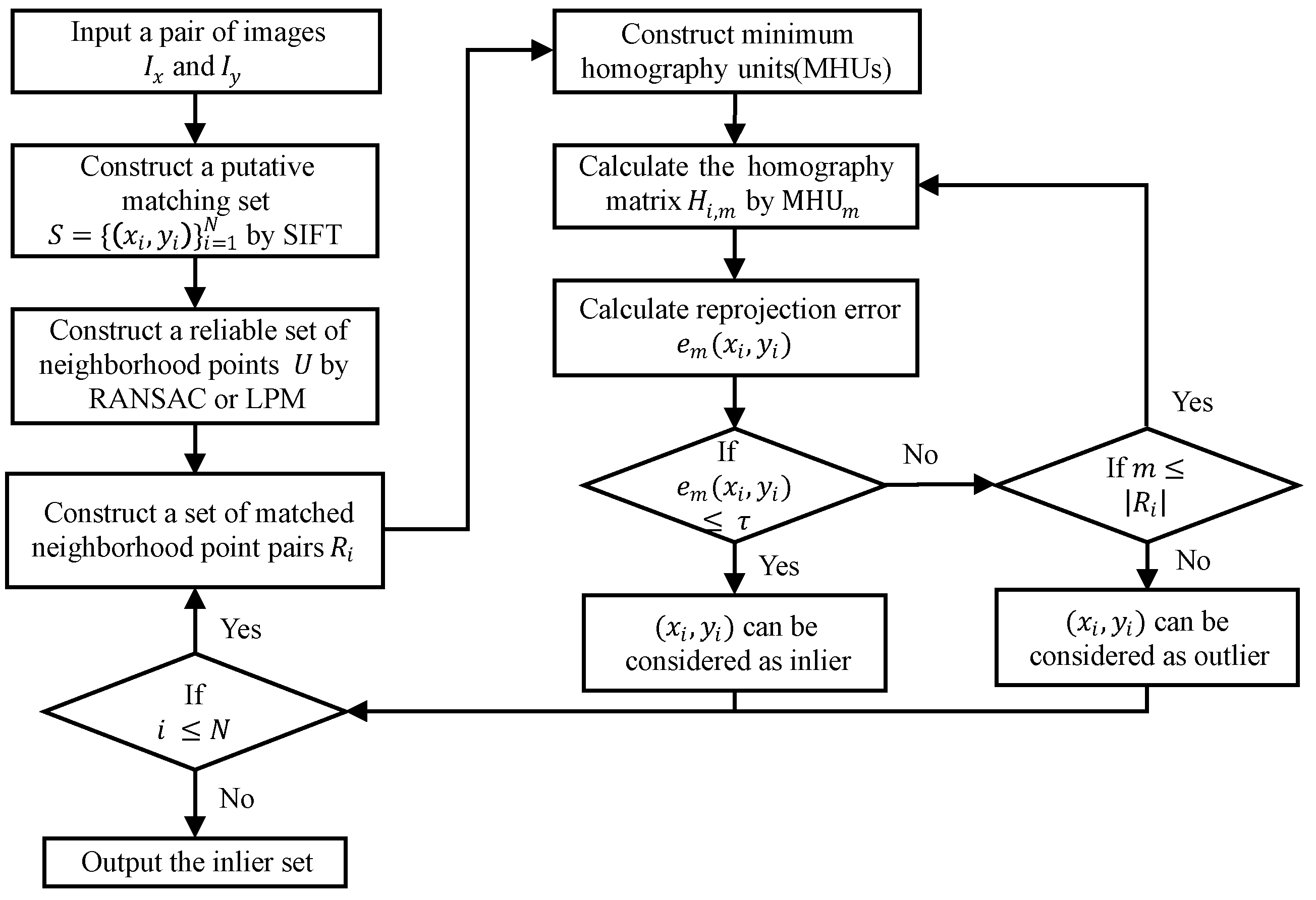
Figure 1. The flowchart of the proposed LMC method.
Remotesensing 15 03379 g001
Figure 2. Illustration of motion consistency and neighborhood topological stability. (a,c) are image pairs I x and I y , where the blue lines connect the correctly matched feature points x i and y i . The yellow lines in (a) represent the connections between feature points and neighboring points when all the neighboring points are inliers. The red lines in (c) represent the connections between feature points and neighboring points when there are outliers among the neighboring points. (b,d) are motion vectors of matches, pointing from x i to y i . (b) is the motion field of correct match vectors, while (c) is the motion field of false match vectors.
Remotesensing 15 03379 g002
Figure 3. MHU structure diagram.
Remotesensing 15 03379 g003
Figure 4. Change curve of algorithm performance under different parameter settings and ablation study.
Remotesensing 15 03379 g004
Figure 5. LMC matching results on 12 image pairs. From top to bottom, the first column shows SUIRD (Horizontal), SUIRD (Vertical), SUIRD (Scaling), and HPatches-i. The second column shows SUIRD (Extreme), SUIRD (Mixture), DTU, and RS (UAV). The third column shows RS (SAR), RS (CIAP), Retina, and RS (PAN). The matching results are presented in the form of image pair matching visualization and motion field of match vectors. True positives are shown in blue, false positives in red, false negatives in green, and true negatives in black. The yellow lines indicate the connections between true positive feature points and their neighboring points. The purple lines indicate the connections between false positive feature points and their neighboring points. To demonstrate the results, only 100 randomly selected matches are displayed, and true negative matches are not shown in the image pairs.
Remotesensing 15 03379 g005
Figure 6. The matching performance of six methods, LPM, mTopKRP, RANSAC, NMRC, LSCC, and LMC, is quantitatively compared on the Extreme, Mixture, and R&S subsets of the SUIRD dataset. The experimental data in Extreme, Mixture, and R&S are shown from top to bottom, and the dataset’s average inlier rate, recall, precision, F-score, and runtime are shown from left to right. Each curve in the figure represents a cumulative distribution. For example, a point ( x , y ) on the LMC curve in the recall plot indicates that the proportion of image pairs with recall less than y for LMC in that dataset is x. All data in the legends are average values, with red indicating the top ranked, blue indicating second ranked, and green indicating third ranked.
Remotesensing 15 03379 g006
Figure 7. A schematic diagram of sorting two image sequences in HPatches-i according to the degree of deformation. From left to right, other images have increasing degrees of deformation relative to the first column image.
Remotesensing 15 03379 g007
Figure 8. Robustness analysis of different methods with an increasing degree of deformation in the HPatches-i dataset.
Remotesensing 15 03379 g008
Figure 9. Seven methods, LPM, mTopKRP, RANSAC, NMRC, LSCC, LMC_RANSAC, and LMC_LPM, are quantitatively compared for their matching performance in five datasets. The experimental data from the DTU, Retina, RS, HPatches, and SUIRD datasets are shown from top to bottom, and from left to right, the data represent the average inlier rate, recall, precision, F-score, and runtime, respectively. Each curve in the graph represents the cumulative distribution. The data shown in all legends represent the average values, with red representing the top ranking, blue representing the second ranking, and green representing the third ranking. When a method is unable to handle image pairs, its recall, precision, and F-score are set to 0 as a penalty, and its runtime is set to 1000 ms.
Remotesensing 15 03379 g009
Table 1. Average precision (AP), recall (AR), F-score (AF), and running time (ART) of all algorithms on three datasets (the red fonts are the maximum values, the blue fonts are the submaximum values).
Method LPMmTopKRPRANSACNMRCLSCCLMC (Ours)
ExtremeAR (%)94.7194.8095.0298.5380.9698.74
AP (%)95.4194.6999.9798.0398.1199.25
AF (%)95.0394.6796.8498.2787.1398.97
ART (ms)14.04860.955.88956.04442.6681.45
MixtureAR (%)95.3896.1697.0799.1284.8199.56
AP (%)96.8996.4899.9798.9298.8499.27
AF (%)96.0596.3198.1899.0288.9499.41
ART (ms)18.621088.456.871281.97727.71107.92
R&SAR (%)96.1896.3296.1698.9984.3899.12
AP (%)96.4396.0299.9898.4298.3899.26
AF (%)96.2896.1297.6498.7089.6799.17
ART (ms)13.63851.734.41949.24415.0083.54
Table 2. Average precision (AP), recall (AR), F-score (AF), and running time (ART) of all algorithms on five datasets (the red fonts are the maximum values, the blue fonts are the submaximum values).
Method LPMmTopKRPRANSACNMRCLSCCLMC_RANSAC (Ours)LMC_LPM (Ours)
DTUAR (%)95.0595.5744.0795.7888.7367.4896.19
AP (%)95.3391.7197.1293.6095.1696.4996.03
AF (%)95.1093.2158.1594.5991.6478.2196.07
ART (ms)10.46650.2233.84739.61451.22326.8595.34
RetinaAR (%)93.7091.8544.9892.0875.9086.2493.92
AP (%)83.1088.2798.0591.5493.0389.5991.06
AF (%)87.6189.3160.6991.5582.8587.7292.24
ART (ms)3.25129.1634.30133.9436.44123.9617.47
RSAR (%)98.8299.2576.8799.2277.5293.4899.10
AP (%)98.1199.0899.5399.1592.9699.5099.22
AF (%)98.4099.1584.7499.1782.2596.0699.16
ART (ms)11.98129.1615.64133.9436.44123.9686.78
HPatchesAR (%)47.4571.0571.5075.2028.4773.7458.91
AP (%)63.5168.1278.8670.4543.3274.1463.77
AF (%)47.5766.3972.7971.2129.7073.3758.57
ART (ms)12.74406.4626.29351.31111.49289.61207.69
SUIRDAR (%)96.4096.6796.2599.1285.4699.2998.06
AP (%)96.7396.4899.9898.6098.5799.2898.03
AF (%)96.5396.5497.7998.8690.3699.2797.92
ART (ms)15.61964.494.64969.60533.9989.5190.70
Disclaimer/Publisher’s Note: The statements, opinions and data contained in all publications are solely those of the individual author(s) and contributor(s) and not of MDPI and/or the editor(s). MDPI and/or the editor(s) disclaim responsibility for any injury to people or property resulting from any ideas, methods, instructions or products referred to in the content.