Abstract
For this study, a new point cloud alignment method is proposed for extracting corner points and aligning them at the geometric level. It can align point clouds that have low overlap and is more robust to outliers and noise. First, planes are extracted from the raw point cloud, and the corner points are defined as the intersection of three planes. Next, graphs are constructed for subsequent point cloud registration by treating corners as vertices and sharing planes as edges. The graph-matching algorithm is then applied to determine correspondence. Finally, point clouds are registered by aligning the corresponding corner points. The proposed method was investigated by utilizing pertinent metrics on datasets with differing overlap. The results demonstrate that the proposed method can align point clouds that have low overlap, yielding an RMSE of about 0.05 cm for datasets with 90% overlap and about 0.2 cm when there is only about 10% overlap. In this situation, the other methods failed to align point clouds. In terms of time consumption, the proposed method can process a point cloud comprising points in 4 s when there is high overlap. When there is low overlap, it can also process a point cloud comprising points in 10 s. The contributions of this study are the definition and extraction of corner points at the geometric level, followed by the use of these corner points to register point clouds. This approach can be directly used for low-precision applications and, in addition, for coarse registration in high-precision applications.
1. Introduction
As 3D sensors, such as laser scanners and depth cameras, have become more widespread, 3D point clouds both indoors and outside can be conveniently collected. Generally, scanning from several angles is required to create a complete 3D model of the object. The collected point clouds must be registered into the global coordinates system as the scanner moves, a process known as point cloud registration. This is a fundamental process in a variety of industries, including robotics [1], unmanned ground vehicles (UGVs) [2], 3D reconstruction [3], and 3D medical imaging [4], among others. A popular approach for aligning two frames of point clouds is to first extract key points from two point clouds and determine the correspondence between them, then estimate the transformation function by aligning the corresponding key points [5]. The least squares approach can be used to theoretically predict an accurate transformation function provided there is no mismatch. However, perfect feature matching is rare even in image processing, which is far ahead of point cloud processing [6].
Despite the fact that point cloud registration has been extensively investigated and different methods for this have been developed, such as iterative closest point (ICP) [7] and its variants [8,9,10,11], sufficient overlap assumption and local minimum issues must still be addressed. In [12], a new point cloud alignment method was developed based on the priors of indoor or similar scene structures, while paper [13] proposed a registration method based on high-level structural information, i.e., plane/line features and their interrelationship, which could overcome the problem of small overlap and increase data collection freedom.
The coarse-to-fine strategy is the most commonly used method for aligning point clouds, where coarse registration is the most difficult. The primary goal of this work is to achieve coarse registration. When establishing a digital model of the environment using a laser scanner, a large number of points will fall on planes or regular surfaces considering that the environment we live in is artificially planned and manufactured, except in the wild. However, the points of interest and utility are frequently situated in the corner or edge areas, making the discovery of a corner or edge point within a 3D point cloud a critical task.
For this study, a new method was proposed to extract corner points at the geometric level, which were then used to align point clouds. Firstly, the corner was defined as the intersection of three planes. Secondly, a graph was constructed with the corners as vertices and the sharing planes as edges. Graph matching was also applied to determine the correspondence between the corners detected from two point clouds. Thirdly, the transformation matrix was calculated by aligning the corresponding corners, and it can then be used to coarsely register the point cloud. Finally, fine registration can be achieved using commonly applied method, e.g., ICP and its variants.
In summary, the main contributions of this paper are as follows:
- (1)
- The definition of the corner point is the intersection of three planes. Both plane/corner detection techniques are included in this study.
- (2)
- A new way of constructing graphs is proposed. The corners are regarded as the vertices and the sharing planes as the edge. Meanwhile, both the distance and angle between linked vertices are taken into account when calculating the affinity matrix. The correspondence is determined using a graph-matching algorithm.
- (3)
- Our method is robust to outliers/noise and can align point clouds that have only a small overlap.
The proposed method is tested on two types of online datasets and compared to other relevant methods in terms of translation and rotation error, root-square-mean error, and run time. The results show that our method can align point clouds that have low overlap and is robust in terms of the quality of the point cloud.
The rest of this paper is structured as follows: Section 2 contains a summary of related work. The methodology is described in Section 3. The datasets and evaluation measures are detailed in Section 4. Section 5 is a presentation of the results. Section 6 is the discussion. Section 7 outlines the conclusions.
2. Related Work
How to align two frames of point clouds has been extensively studied in the fields of computer vision, computer graphics, and robotics [14,15,16]. The general method is based on a coarse-to-fine strategy. For the fine step, it can be completed by ICP (iterative closest point) [7] and NDT (normal distribution transform) [17] or their variants [8,10,18]. Most recent studies focus on the coarse step, which provides the initial estimation for the fine step. This paper also focuses on the coarse registration of point clouds, which can be roughly divided into two categories: correspondence-based methods and non-correspondence-based methods.
Correspondence-based registration involves determining the correspondence between two point clouds and then calculating the transformation matrix. It can be divided into two categories: finding the correspondence on the raw point clouds and on the keypoints [19,20,21,22]. In the first, the nearest neighbor is usually regarded as the corresponding point as in ICP [7]. For the second, key points are extracted, and a recognizable descriptor is then designed to describe them. The corresponding points are those whose descriptions are most similar. Our work follows the keypoint-based method.
ICP is a widely used correspondence-based method, and many improved versions have emerged since its proposal. Generalized-ICP [23] improves the robustness of ICP by incorporating probability modules into its framework. Go-ICP [24] is a globally optimal version of ICP that addresses the disadvantage of ICP being prone to falling into local minima. All these methods have overcome some disadvantages of ICP but are sensitive to the initial estimation.
Non-correspondence-based registration is robust to missing correspondence and outliers, because it is not based on the assumption of correspondence [25]. NDT (normal distribution transform) [17] projects points into cells and computes the PDF (probability density function) of each cell. The best transformation maximizes the likelihood function. GMMREG [26] redefines registration as the alignment of two Gaussian mixture models, which is an optimization problem, to minimize the distance between the two models. CPD (coherent point drift) [27] is a probabilistic-based registration for rigid and nonrigid objects. The registration is defined as the MLE (maximum-likelihood estimation) and solved using an EM (expectation-maximization) strategy. GMMREG and CPD cannot often be used to process large-scale data because of the requirement to calculate the pairwise point distance of two point sets. ECPD (extended coherent point drift) [28] couples correspondence into registration to process large-scale point sets. In FilterReg [29], the E-step is replaced with a filter to accelerate alignment. However, these methods are unable to overcome the problems caused by small overlaps and occlusion.
Learning-based registration, which has recently been widely studied, involves use of an end-to-end approach to estimate the transformation matrix directly. However, these methods are vulnerable to outliers, which often leads to incorrect correspondence. Reference [30] proposed a deep graph-matching framework to reduce the correspondence error. PRNet [31] uses deep networks to tackle the alignment non-convexity and the partial correspondence problem. RPM-Net [32] is a more robust deep learning-based method that overcomes the disadvantage of ICP in being easily influenced by outliers.
3. Methodology
The methodology is organized into three steps. First, planes are extracted from the raw point cloud, and corners are obtained by intersecting three planes. Second, a graph is constructed, and a graph-matching algorithm is utilized to identify the correspondence between the corners of two point clouds. Finally, the point clouds are coarsely registered by aligning the appropriate corners, then refined using point-to-plane ICP. Figure 1 depicts the whole framework of this study.
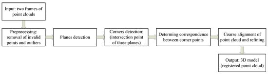
Figure 1.
The overall framework of this paper.
3.1. Plane Detection
The plane and corner are the basic primitives of the point cloud for many developed detection algorithms. These methods can be categorized as HT (Hough transform) [33], RANSAC (RANdom SAmple Consensus) [34], and region-growing [35,36]. For HT, the voting is computationally expensive. Although some strategies have been proposed to accelerate plane detection, it cannot be guaranteed that all planes, especially small ones, can be detected. RANSAC is easy to implement and robust to noise. Because of the random approach, however, it always fits a plane that does not really exist. An octree-based region-growing approach was proposed in the literature [36] to detect planes. Although effective, it depends on the threshold: residual . Additionally, it depends on the precision of the normals, which are typically estimated by PCA (principal component analysis), a method that is susceptible to outliers. DBSCAN (density-based spatial clustering of applications with noise) [37] is a representative density-based clustering algorithm that may detect clusters of any shape and does not require a predetermined number of clusters to be produced.
In this study, DBSCAN is adopted to detect planes, where it was run on a Gaussian sphere to cluster planes with similar normals and then again on points in the cluster to distinguish individual planes. The details are described in the following.
3.1.1. Gaussian Sphere
In Gaussian mapping, point clouds are projected onto a Gaussian sphere, allowing intuitively reflecting the distribution of the point normals [38]. Let the point cloud be denoted as a point set , the kNN (k-nearest neighbors) of be , , where are the Cartesian coordinates of . The normal of can then be estimated by performing PCA on the kNN, and the steps are: (1) calculating the kNN’s covariance matrix using Equation (1); (2) performing EVD (eigenvalue decomposition) on ; (3) sorting the eigenvalues; and (4) determining the ’s normal, which is the eigenvector corresponding to the minimum eigenvalue.
where is the mean of the point coordinates.
The mean estimator is particularly vulnerable to outliers from the perspective of robust estimation [39], whose breakdown is , where n is the number of samples. It is obvious that the breakdown converges to as . Thus, the median estimator, which has a breakdown value of and is robust to outliers, is used in place of the mean estimator. Then, the covariance matrix is calculated using Equation (2):
where is the median of points’ coordinates.
The normals can be estimated more precisely by substituting the median estimator for the mean estimator. However, the estimated normal has an ambiguity of . Hence, the MST (minimum span tree) [40] is used to orient the normals. The estimated normals of the point cloud can also be denoted as a point set, , where is the normal of . Then is the projection of on the Gaussian sphere.
3.1.2. Plane Detection
It is challenging to extract planes by running the DBSCAN algorithm directly on the point cloud, in which points are clustered based only on Euclidean distance. All points that fulfill density reachability are grouped into the same cluster regardless of whether or not they are on the same plane. When transplanting DBSCAN to the Gaussian sphere, points on the same plane or other parallel planes would be grouped into the same cluster, since they have similar features of normals.
Some parameters and definitions of DBSCAN are as follows:
Parameters: , the radius of the searching neighborhood, and , the minimum number of points.
Types of points: core, border, and noise points. Given a point p, its neighbors within radius are and the number of neighbors is .
- Core: If , then p is core points. All points in are grouped into the same cluster.
- Border: If a point q has been grouped into a cluster but is not a core point, then it is a border point.
- Noise: If a point q is neither a core point nor a border point, then it is a noise point.
Density directly attainable: If p is a core point and , the density can be directly obtained from p to q.
Density attainable: If the density is directly attainable from p to and from to q, then the density can be obtained from p to q.
Density connected: If the density is attainable from to p and from to q, then the density is connected between p and q.
Density non-connected: If no points cause p and q density to be connected, then they are density non-connected.
Despite the fact that the DBSCAN on a Gaussian sphere can group coplanar points—those with similar normals—into a single cluster, it is unable to separate apart points on parallel planes. To illustrate the process of plane detection, a point cloud was acquired by an RGB-D camera, as shown in Figure 2a. The projection of the point cloud onto the Gaussian sphere is shown in Figure 2b. After projecting the point cloud onto the Gaussian sphere, the DBSCAN is performed to cluster the points with similar normals. The result of clustering on the Gaussian sphere is shown in Figure 2c, and the corresponding points in Euclidean space are shown in Figure 2d. It can be seen that the points on the different parallel planes (blue points in Figure 2d) were grouped into the same cluster. To identify the planes within a cluster, DBSCAN was once more performed on the points belonging to the same cluster in Euclidean space, because there must be a density gap if a cluster contains multiple parallel planes. The details of plane detection are shown in Algorithm 1.
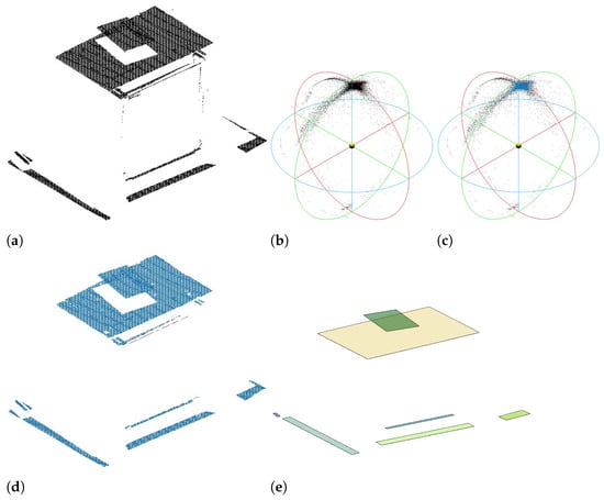
Figure 2.
The process of plane detection. (a) shows the raw point cloud. The projection on the Gaussian sphere is shown in (b) and the clustering result is shown in (c). (d) shows the points in Euclidean space corresponding to the clustered points in (c). (e) is the detected planes extracted from (d).
The detected plane was represented as a rectangle with three attributes: vertices, center, and normal. To obtain the model of the detected plane, a PCA (principal component analysis)-based method was designed to calculate the plane parameters. Given a set of coplanar points P, P was then projected into the feature space that was acquired by PCA. The process of plane fitting is shown in Algorithm 2. The detected planes are shown in Figure 2e.
| Algorithm 1: Plane detection by DBSCAN |
 |
| Algorithm 2: fitPlanePCA(P) |
Input: Colanar points: Output: Model of plane: , ▹ Normalization; ▹ Calculating covariance matrix; ▹ Basis of feature space; ▹ Projecting P into feature space; , , , , ▹ The vertices are A, B, C, and D; ▹ Re-projecting vertices into Euclidean space; return |
3.2. Corner Detection
In contrast to the typical key points, this paper extracts the corner points where the three planes intersect. The smallest rectangle containing all planar points is used to represent the detected plane. Let a detected plane be , and the normal, center, and vertices of be , respectively. To obtain the intersection of three planes, the plane was denoted as its parametric Equation (3).
where .
Given three planes, , they can also be represented as homogeneous form: , where and . Then , , and intersect at a point if . The coordinate of the intersection point can be calculated easily by .
In this way, a set of corner points can be obtained. However, some are invalid. To find and discard invalid intersections, the distances from the corner point to three intersected planes are calculated and compared based on a predefined tolerance ; i.e., if both distances are not larger than , the corner point is valid.
In addition, the intersecting planes cannot be guaranteed to be orthogonal, and the edges of a plane cannot be guaranteed to be parallel to the intersection line, as shown in Figure 3a. Given three planes () and a corner point (P), P is valid if and only if it is inner for all three planes.
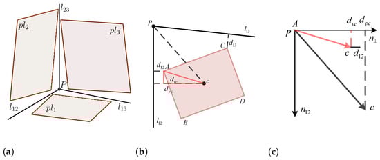
Figure 3.
Illustration showing the position of the intersection point and three planes: (a) the position of the corner and three intersecting planes, (b) the position of the corner and one of the intersecting planes, and (c) the calculation of the distance from the center of a plane to the intersection line.
Taking the calculation of the distance from point P to plane as an illustration, in Figure 3b, is the intersection line of and , is the intersection line of and , is the distance from to , and is the distance from to . To calculate , the nearest vertex to line should first be located; for instance, A is the closest to in Figure 3b. Then is defined as the distance from A to . The vector is translated by vector as shown in Figure 3c, where is the vertical vector of . If , line intersects with plane . Otherwise, if , line also intersects with plane . The same procedure can be used to assess whether or not line intersects with plane . If and only if and intersect with , P is inner for . The location between P and planes is determined in the same way. P is valid if and only if it is inner for planes . In conclusion, the method of corner detection is shown in Algorithm 3.
The value of is set to be 0.1 times the diagonal length, i.e., , in this study. The corner detection algorithm proposed in this study is performed on the point clouds and from dataset Apartment, and the results are shown in Figure 4. It is obvious that the corners found by the proposed algorithm are at the geometric level, as opposed to the corners detected by traditional algorithms, such as Harris 3D, among others.
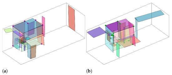
Figure 4.
Planes and corners detected from and of the dataset Apartment are depicted in (a) and (b), respectively.
3.3. Registration
Registration is a simple but crucial step in the processing of point clouds. It depends on the assumption that there is correspondence between two clouds. However, in practice, such correspondence between the point clouds gathered at various times is either absent or challenging to find. In this study, graph matching is employed to identify the corners’ correspondence.
A graph G, including directed and undirected graphs, can be represented as , where and are the set of vertices and edges, respectively. And , are the i-th vertex and edge. The graph is complete graph if there are edges linking any two vertices. In this study, is defined as the previously detected corners. As the corners are obtained through the intersection of three planes, edges exist only between corners sharing a sharing plane. Figure 5 shows graphs formed by corners detected from and of the dataset Apartment.
| Algorithm 3: Corner detection |
 |
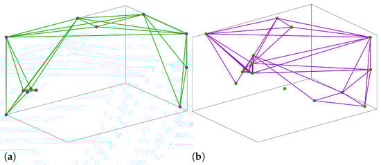
Figure 5.
Illustration of graph construction. The graph formed by and are depicted in (a) and (b), respectively.
The aim of graph matching (GM) is to determine the correspondence between the nodes of two graphs. As is known, graph matching can be used to address feature matching in computer vision. Let two undirected graphs be and with size of m and n, respectively. The affinity matrix is employed to measure the similarity between each pair of edges; e.g., measures the similarity between edges and when corresponds to , respectively. The goal of GM is to identify the optimal assignment/permutation matrix that will maximize the similarity of nodes and edges between two graphs, where means corresponds to and otherwise. Equation (4) defines GM as an integer quadratic program (IQP), meaning that the scoring function is maximized by the indicator vector .
where the constraints guarantee one-to-one matching from to . The approximation approach is used to resolve the NP-hard problem of IQP in terms of implementation. The RRWM [41] method was used in this study.
By constructing an association graph, RRWM interprets the GM between and as a random walk issue. The association graph is defined as , which regards a pair of corresponding nodes and as its node, where and . The similarity metric is the associated weight. Now, the main task is to calculate the affinity matrix that includes two similarity metrics, distance and angle.
Distance metric: Let , be the distances between . If match , and are similar, i.e., . The affinity matrix of distance is calculated using Equation (5):
where is the scaling factor and is set to . It can be seen that when , ; otherwise, .
Angle metric: Let be the angle between vectors and . If match , vectors and are approach parallel, i.e., . Then the affinity matrix of angle is calculated using Equation (6):
where .
That is, when the vectors and approach parallel, .
Affinity matrix: can be calculated by combining and by means of simple weighting, as shown in Equation (7):
where k is the weight of . The ratio of and in can be adjusted by tuning the value of k. It is worth noting that both three matrices should be normalized, e.g., is normalized by .
Matching: RRWM [41] treats the associate graph as a Markov chain. The process of matching between two given graphs is thus regarded as the node ranking and selection by random walks in the association graph. Affinity-preserving random walk converts affinity matrix to a transition matrix by , where and . When preserving affinity random walk, RRWM takes into account two-way constraints as shown in Equation (4).
For the random walker, a probability distribution will be obtained at each time , which can be denoted as . Then is updated by , where is the reweighted jump vector and calculated by . The parameters and are usually set to and 30. Random walks are iteratively conducted on and probability is updated until converges, i.e., . Finally, the probability is discretized by the Hungarian algorithm [42] to determine the correspondence between two graphs and .
After finding the correspondence between two point clouds, as shown in Figure 6, SVD (singular value decomposition) can then be used to solve the transformation matrix after identifying the correspondence between two point sets (corner points in this case).
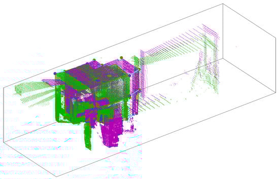
Figure 6.
The correspondence obtained by GM. Point clouds and are colored in magenta and green, respectively. To ensure clarity of the visualization, the corner points extracted from and are colored in green and magenta, and the corresponding corner points are linked by the thick, solid cyan line.
Assume two point clouds are and , which are called source and target data, respectively. The corresponding corner points extracted from and are and , and corresponds to . The issue of alignment is to find a transformation matrix such that
where is the rotation matrix and is the translation vector.
The details of the transformation matrix calculation are established in [43]. The following is a list of the main steps:
- (1)
- The corner points are centralized by , , where , , and k is the number of matched corner points;
- (2)
- The covariance matrix is calculated by ;
- (3)
- SVD (singular value decomposition) is performed on , which can be written as . The rotation matrix is ;
- (4)
- Finally, translation can be calculated by .
Once the transformation matrix has been obtained, the source point cloud can be transformed into the same coordinate system as the target point cloud by . The transformed point cloud can be used as an input for fine registration.
In general, fine registration after coarse registration is essential to more precisely align two point clouds. ICP (iterative closest point), including point-to-point and point-to-plane, is the technique frequently employed for fine registration. The closest point pair is used as a correspondence in point-to-point ICP. Then, transformation is determined by minimizing the sum of the Euclidean distance between the point pairs. Point-to-plane ICP replaces point-to-point distance with point-to-plane distance due to the limits of this correspondence. Its optimization objective is to minimize the total orthogonal distances between the points in the source point cloud and the corresponding local planes in the target point cloud.
This study will employ point-to-plane ICP for fine registration and compare the results of the registration.
4. Materials and Evaluation
The purpose of this study is to register indoor 3D point clouds. To verify the applicability of the proposed method, two types of datasets with various resolutions were selected, one of which was acquired by Hokuyo rangefinder UTM-30LX and the other by Riegl VZ-400. The former has a significant overlap rate, while the latter has a very low overlap rate. In each type of dataset, two point clouds with different scales are chosen, i.e., Apartment, Stairs from Hokuyo and ThermalMapper, ThermoLab from Riegl.
4.1. Datasets
Hokuyo: Two datasets recorded by Hokuyo, Apartment and Stairs [44], can be accessed on the homepage of ASL (Autonomous System Lab) (https://projects.asl.ethz.ch/datasets/, accessed on 19 October 2022). “Apartment” is collected in Kilchberg, Zurich, Switzerland, and intended for testing the robustness of the registration algorithm against outliers and dynamic objects. A laser rangefinder (Hokuyo UTM-30LX) (https://www.hokuyo-aut.jp/search/single.php?serial=169download, accessed on 19 October 2022) is mounted on a tilting device to acquire the range of the measured object. The ground truth of the transformation matrix () is listed in icpList.csv, which is used to compute the errors. It is worth noting that each aligns the corresponding point cloud to . However, we aligned the current frame to the previous frame . Hence, when calculating the errors, we need to operate the transformation matrices by such that the calculated T is consistent with the T in the ground truth. There are a total of 45 and 31 scan frames in datasets Apartment and Stairs, respectively. Their first two scans are shown in Figure 7, where those in magenta are the first scans and those in green are the second scans.
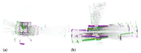
Figure 7.
Illustration of the first two scans of the datasets Apartment (a) and Stairs (b). The magenta ones are the first scans and the green ones are the second scans.
Riegl: Two datasets obtained by Riegl VZ-400 (http://www.riegl.com/nc/products/terrestrial-scanning/, accessed on 19 October 2022) can be found on the website of Robotic 3D Scan Repository (http://kos.informatik.uni-osnabrueck.de/3Dscans/, accessed on 19 October 2022), which are referred to as ThermalMapper and ThermoLab. The raw data also include infrared data acquired by IR (infrared) in addition to the XYZ coordinate information used in this study. ThermalMapper is recorded as part of the ThermalMapper project by Jacobs University Bremen, including 3D scans of the inside and outside of a German residential home, and only the inside views are used in this study. ThermoLab is collected in the Automation Lab at Jacobs University Bremen. There are seven and seventeen frames of point clouds in ThermoLab and ThermalMapper, respectively, which were collected at various poses. To generate a 360-degree scan, nine 40-degree scans are included in each frame. The file scanXXX.frames contains the ground truth of the pose, which is estimated by odometry data and refined by slam6d (https://slam6d.sourceforge.io/, accessed on 19 October 2022). Their first two scans are shown in Figure 8.
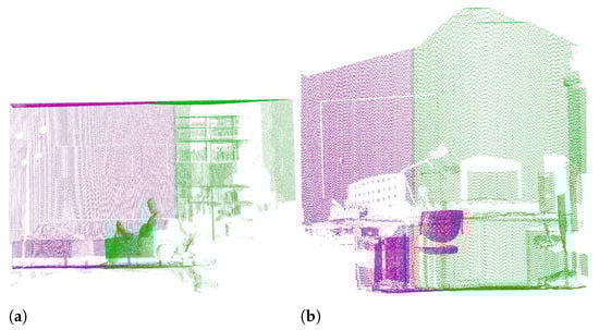
Figure 8.
Illustration of the first two scans of the datasets Thermalmapper (a) and ThermoLab (b). The magenta ones are the first scans and the green ones are the second scans.
For brevity, we refer to the datasets Apartment, Stairs, Thermalmapper, ThermoLab in the following by the abbreviations DS-1, DS-2, DS-3, DS-4, respectively. Their details of them are summarized in Table 1. “NO. of frames” represents the number of scans at various poses, where implies n frames of point cloud, each frame consists of nine scans (). “Avg. points” is the approximate number of points per frame. The “Resolution” is determined by the average distance between each point and its nearest neighbor, i.e., . “Scale” refers to the size of the global map, where “small” and “large” are relative, rather than absolute, concepts. It is notable that the outliers (noise) are included in “NO. of points” but removed when calculating “Resolution”.

Table 1.
Details of the datasets used in this study.
4.2. Evaluation
The common evaluation criteria of point cloud registration algorithms are the RMSE (root-mean-square error) and the rotation/translation error ().
When calculating RMSE, we employ two point clouds that correspond one by one, one of which is transformed by the ground truth transformation matrix and the other by the transformation matrix that was estimated in this study. RMSE is the average Euclidean distance between the corresponding points. It can also be used to judge whether the registration is successful, i.e., if the RMSE is larger than a preset threshold, the registration is considered to have failed. The calculation of RMSE is shown in Equation (9):
where , are the ground truth of the rotation matrix and translation vector, and , are the estimated ones, is a point in the point cloud, and N is the point number. Moreover, when there is no ground truth, the nearest neighbor point is commonly used to calculate the RMSE.
Rotation error evaluates the rotation angle difference between the estimated and the ground truth of the rotation matrices and is calculated using Equation (10). Translation error evaluates the error between the ground truth and the estimated translation vectors and is calculated using Equation (11).
where means “ground truth”, R is the rotation matrix, is the translation vector, and the transformation matrix consists of rotation and translation: .
Let the n point clouds that were acquired at different poses be denoted by and the reference frame be , then represents the transformation from to . can be calculated by . By transforming all point clouds to , a 3D model of the measuring object can be created. Meanwhile, these transformation matrices can be used to estimate the pose of the sensor.
5. Results
The following experiments were performed on a laptop running Ubuntu 20.4 LTS with Ryzen R7 processor, 16 GB of RAM, and 512 GB SSD. All experiments were processed on the raw data without voxelization or any other downsampling processing.
For brevity, ICP1 and ICP2 are the point-to-point and point-to-plane ICPs [7,9]. NDT means the normal distribution transform [17]. GICP represents the Generalized-ICP [23], FGICP represents the fast-GICP [45], and KFPCS represents the keypoint-based 4PCS [46] in the following figures and tables. In terms of parameter setting, the allowable variation of the transformation matrix is set to 0.001 to decide whether or not to stop iteration for ICP1, ICP2, and NDT, and the weight factor is set to 0.1 for KFPCS. For all fine registration, ICP2 was applied.
To demonstrate the feasibility of the method proposed in this study, a subset of about 30,000 points was selected from of the dataset DS-1, which are the magenta points in Figure 9a. It was then transformed by a preset transformation matrix, which are the green points in Figure 9a. We compared the registration with some commonly used classic methods, i.e., ICP1, ICP2, NDT, KFPCS, GICP, and FGICP, as shown in Figure 9b–h. Then, the metrics RMSE, , and were calculated and are listed in Table 2.
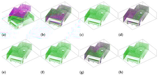
Figure 9.
The magenta points are the subsets of point cloud from DS-1, and the green points are the transformed point clouds: (a) the points before alignment and (b–h) the registration results of methods ICP1, ICP2, NDT, GICP, FGICP, KFPCS, Proposed, respectively.
Table 2.
Performance comparison of different methods on the subset of point cloud from DS-1. The metrics of fine registration are the same as for ICP2.
It is worth noting that the selected subset selected must guarantee at least three corner points can be detected such that a unique matrix can be determined when [47].
The proposed method was evaluated on two indoor datasets of different scale, DS-1 and DS-2, and compared with the aforementioned algorithms on the basis of errors and time consumption, as shown in Figure 10. As described in Table 1, these two datasets have high overlap and low resolution. The dataset DS-1 and registration results of the corresponding method are shown in Figure 10a. It can be seen that NDT fails to align the two point clouds. The dataset DS-2 and registration results of the corresponding method are shown in Figure 10b. It can be seen that the results of NDT are still the worst. The errors and time consumption are listed in Table 3.
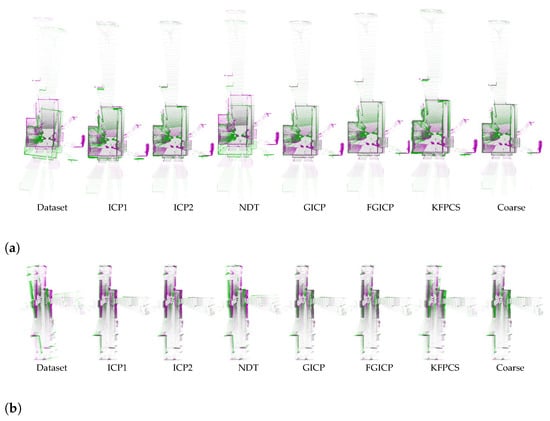
Figure 10.
Registration results of different methods on the datasets DS-1 (a) and DS-2 (b), where and are colored in magenta and green, respectively.
Table 3.
Performance comparison of aligning to from DS-1 and DS-2 using the aforementioned methods. DS1 and DS2 represent the datasets DS-1 and DS-2, respectively. The metrics of fine registration are the same as for ICP2. The optimal and suboptimal evaluation indicators are written in bold and italics, respectively.
To demonstrate the superiority of the proposed method, two datasets with high resolution but low overlap were used, which are datasets acquired by Riegl. Riegl can acquire 3D point clouds with good accuracy up to 800 m. For this dataset, both the aforementioned algorithms were unable to align the point clouds due to the minimal overlap. The registration results of the proposed method are shown in Figure 11. Figure 11a shows the coarse and fine registration of the dataset DS-3, and Figure 11b shows the coarse and fine registration of the dataset DS-4. The metrics of the proposed method are shown in Table 4, where ICP2 was used for fine registration. In Table 4, the denotation of “” is the metrics of coarse (a) and fine (b) registration.
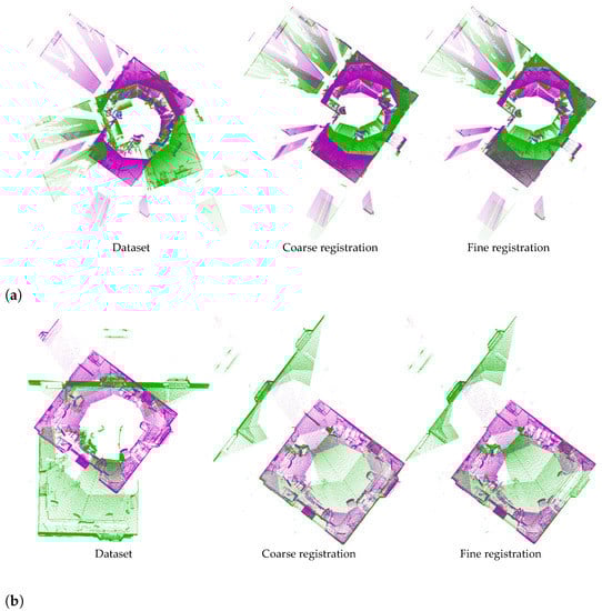
Figure 11.
The registration results of the proposed method conducted on datasets DS-3 (a) and DS-4 (b). Those in magenta are the first frames and those in green are the second frames. The first frame consists of scan000 to scan008 and the second consists of scan009 to scan017. ICP2 is used for fine registration.
Table 4.
Performance of the method proposed in this study to aligning to from DS-3 and DS-4. The first frame consists of scan000 to scan008 and the second consists of scan009 to scan017.
Figure 12 shows the global maps of the four datasets and scanner poses in the map. As described in Table 1, the four datasets (DS-1, DS-2, DS-3, DS-4) contain 45, 31, 17, 7 frames of point clouds, respectively. A global map can be obtained by aligning all of the point clouds to the same reference frame, as shown in Figure 12a. Meanwhile, the pose transformation is implied in the process of point cloud registration. As shown in Figure 12b, let the point cloud acquired at be and the one acquired at be . After transforming to the reference frame of , i.e., , the pose transformation can then be represented as , where and , is the transformation matrix, is the rotation matrix, and is the translation vector, and is usually set to .
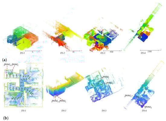
Figure 12.
Global maps (a) of the four datasets and the scanner poses (b) during the acquisition of each point cloud.
For the four datasets, the errors were calculated for each pose. The error is the Euclidean distance between the estimated and ground truth of the pose. The proposed method is compared to the aforementioned methods on datasets DS-1 and DS-2, as shown in Figure 13a,b. Figure 13c shows the errors calculated only by the proposed method because alignment failed when using the aforementioned methods.
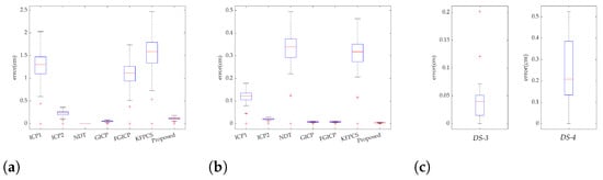
Figure 13.
The pose errors of the four datasets. (a,b) show the errors of different methods on DS-1 and DS-2, respectively. (c) only shows the errors of the proposed method on DS-3 and DS-4 because the other methods failed to align point cloud.
The proposed method was tested on the point clouds obtained by an RGB-D camera, another popular point cloud acquisition tool, to confirm its applicability. The popularization of RGB-D cameras, e.g., Microsoft Kinect, Asus Xtion Live, Intel RealSense, Google Tango, and Occiptial’s Structure Sensor, makes it convenient to obtain 3D point clouds. However, compared to the point clouds acquired by LiDAR, those acquired by these cameras are low quality, because they are sensitive to the shininess, brightness, and transparency of surfaces [48]. Additionally, RGB-D cameras have a limited range, e.g., 0.8–2.5 m for Kinect v2. The dataset is selected from Redwood [49] (Redwood: https://codeload.github.com/isl-org/open3d_downloads/tar.gz/refs/tags/RGBD, accessed on 5 July 2021). The raw point clouds, the coarsely and finely aligned point clouds are shown in Figure 14. Due to the lack of ground truth, the nearest neighbor of is treated as its corresponding point if the distance between them is less than a threshold , which is set as 0.007 in this study. Only RMSE was calculated and written in the northeast of figures for the coarse and fine registration in Figure 14b.
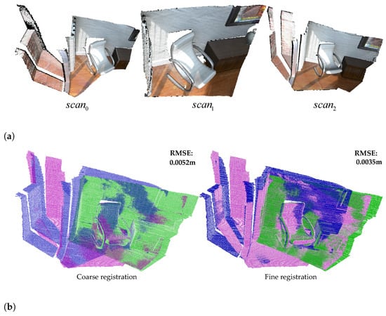
Figure 14.
Performing the proposed method on the point clouds acquired by an RGBD camera. (a) shows the raw point cloud. (b) is the results of coarse and fine registration, where the points in are colored in magenta, green, and blue, respectively.
6. Discussion
The results in Section 5 show that the proposed method can align point clouds with acceptable time consumption. Although it was used for the coarse registration in this study, its performance is close or even superior to point-to-point ICP. Moreover, it has mild overlap constraints compared to other algorithms (at least those mentioned above).
First, a dataset containing actual one-to-one communication was used to test the suggested method and the aforementioned methods. The target point cloud is a subset of the first scan of DS-1, and the source point cloud is obtained by transforming the target point cloud with manually set rotation angle and translation vector, as shown in Figure 9a. Figure 9b–h are the registration results of the algorithms ICP1, ICP2, NDT, GICP, FGICP, KFPCS, and the proposed method, respectively. Table 2 lists the relevant metrics of the aforementioned methods. Due to the presence of one-to-one correspondence and high overlap, all methods can accurately align point clouds.
Secondly, two datasets with high overlap but lacking one-to-one correspondence were used to validate the proposed method, as shown in Figure 10. Table 3 lists the relevant metrics of the algorithms. It can be seen that, in terms of accuracy, GICP and FGICP demonstrate the best performance, followed by the proposed method with the submillimeter RMSE . However, in terms of runtime, the proposed method is slightly inferior to FGICP and much faster than GICP.
Thirdly, two datasets with low overlap and lacking one-to-one correspondence were used to verify the superiority of the proposed method, as shown in Figure 11. All the aforementioned algorithms failed to align point cloud because of the low overlap. Hence, Table 4 lists only the metrics of the proposed method. The suggested method can achieve centimeter-level accuracy (RMSE) during the coarse registration stage and millimeter-level accuracy after fine registration.
Finally, we built the global maps for datasets DS-1, DS-2, DS-3, and DS-4, by aligning all their point clouds, and calculated the error at each sampling point. The global maps are shown in Figure 12a, and the poses of the scanner in the map are shown in Figure 12b. Meanwhile, Figure 12b indicates the sampling poses of the scanner for acquiring the four datasets (DS-1, DS-2, DS-3, DS-4), means the pose of scanner for acquiring point cloud . The errors are shown in Figure 13 in the form of a boxplot, where the top and bottom of each box are the 75th and 25th percentiles of the errors, the red lines are the median of errors, the whiskers extend to the upper/lower limits of errors, and red ‘+’ signs are considered outliers.
In addition, the dataset acquired by the RGB-D camera was used to test the applicability of the proposed method, which is of low quality due to the physical characteristics of the sensor. Figure 14a shows the raw point clouds, and Figure 14b shows the registration results of the proposed method. In the northeast corner of each in Figure 14b, the corresponding value of RMSE is recorded. As seen, the RMSE value also reaches the millimeter level.
In terms of time consumption, the proposed method spends more time on coarse registration or, more specifically, on planar detection. As shown in Table 2, Table 3 and Table 4, even when point clouds have a scale of up to millions, our method can align them in a few tens of seconds (at most).
In summary, the proposed method has a weak constraint regarding the overlap and is robust to data quality. Our method is nevertheless useful when other algorithms cannot align lowly overlapping point clouds, even though it is slightly inferior to the FGICP when there is large overlap between point clouds. It is worth noting that for our method, there is still the requirement that at least three corresponding corners can be detected in the point clouds to be registered. In addition, the method is suitable for registration of 3D point clouds acquired in structured environments, because it aligns corner points produced by the intersection of three planes.
7. Conclusions
In this paper, we present a new method for aligning indoor 3D point clouds. Firstly, the planes are detected and the corner points are defined as the intersection of three planes. Secondly, a graph is constructed with the corner points as vertices and the sharing plane as edges. The distance and angle metrics are defined and adopted to calculate the affinity matrix. RRWM is then employed to determine the correspondence. Finally, coarse registration was achieved through SVD, and fine registration was fulfilled by point-to-plane ICP.
The advantages of our method are summarized in the following.
- (1)
- Low overlap: Because it aligns the corners defined on the geometric level rather than the real point cloud in the rough alignment stage.
- (2)
- Fast: The number of corners is limited, so it is very fast to align them. Most of the time is spent on plane detection.
- (3)
- Robust: It can process various point clouds acquired by different sensors.
However, it is necessary to ensure that at least three corresponding corner points can be detected in the point clouds to be registered. In addition, our method was tested on the indoor datasets. When geometric information is insufficient, such as outside or in the field, the method might not be appropriate.
Author Contributions
Conceptualization, W.W. and G.G.; methodology, W.W.; software, W.W. and H.Y.; validation, W.W., Y.W. and G.G.; formal analysis, G.G.; investigation, W.W.; resources, W.W.; data curation, G.G.; writing—original draft preparation, W.W.; writing—review and editing, G.G. and H.Y.; visualization, W.W.; supervision, Y.Z.; project administration, Y.Z.; funding acquisition, Y.W. and G.G. All authors have read and agreed to the published version of the manuscript.
Funding
This research was sponsored by the National Key Research and Development Program (2020YFB1710300), Aeronautical Science Fund of China (2019ZE105001), and the Research Project of Chinese Disabled Persons’ Federation on assistive technology (2022CDPFAT-01).
Data Availability Statement
Links to the original datasets have been added where they first appear in the text. The results of this study are available on request from the corresponding author.
Acknowledgments
We sincerely appreciate the authors for providing the datasets and the advice from editors and reviewers.
Conflicts of Interest
The authors declare no conflict of interest.
References
- Kim, P.; Chen, J.; Cho, Y.K. SLAM-driven robotic mapping and registration of 3D point clouds. Autom. Constr. 2018, 89, 38–48. [Google Scholar] [CrossRef]
- Wu, Y.; Li, Y.; Li, W.; Li, H.; Lu, R. Robust LiDAR-based localization scheme for unmanned ground vehicle via multisensor fusion. IEEE Trans. Neural Netw. Learn. Syst. 2020, 32, 5633–5643. [Google Scholar] [CrossRef] [PubMed]
- Xu, H.; Yu, L.; Hou, J.; Fei, S. Automatic reconstruction method for large scene based on multi-site point cloud stitching. Measurement 2019, 131, 590–596. [Google Scholar] [CrossRef]
- Fu, Y.; Lei, Y.; Wang, T.; Patel, P.; Jani, A.B.; Mao, H.; Curran, W.J.; Liu, T.; Yang, X. Biomechanically constrained non-rigid MR-TRUS prostate registration using deep learning based 3D point cloud matching. Med. Image Anal. 2021, 67, 101845. [Google Scholar] [CrossRef] [PubMed]
- Tam, G.K.; Cheng, Z.Q.; Lai, Y.K.; Langbein, F.C.; Liu, Y.; Marshall, D.; Martin, R.R.; Sun, X.F.; Rosin, P.L. Registration of 3D point clouds and meshes: A survey from rigid to nonrigid. IEEE Trans. Vis. Comput. Graph. 2012, 19, 1199–1217. [Google Scholar] [CrossRef]
- Tombari, F.; Salti, S.; Di Stefano, L. Performance evaluation of 3D keypoint detectors. Int. J. Comput. Vis. 2013, 102, 198–220. [Google Scholar] [CrossRef]
- Besl, P.J.; McKay, N.D. A Method for Registration of 3-D Shapes. IEEE Trans. Pattern Anal. Mach. Intell. 1992, 14, 239–256. [Google Scholar] [CrossRef]
- Chen, Y.; Medioni, G. Object modelling by registration of multiple range images. Image Vis. Comput. 1992, 10, 145–155. [Google Scholar] [CrossRef]
- Grant, D.; Bethel, J.; Crawford, M. Point-to-plane registration of terrestrial laser scans. ISPRS J. Photogramm. Remote Sens. 2012, 72, 16–26. [Google Scholar] [CrossRef]
- Bouaziz, S.; Tagliasacchi, A.; Pauly, M. Sparse Iterative Closest Point. Comput. Graph. Forum 2013, 32, 113–123. [Google Scholar] [CrossRef]
- Rusinkiewicz, S. A symmetric objective function for ICP. ACM Trans. Graph. 2019, 38, 1–7. [Google Scholar] [CrossRef]
- Sanchez, J.; Denis, F.; Checchin, P.; Dupont, F.; Trassoudaine, L. Global registration of 3D LiDAR point clouds based on scene features: Application to structured environments. Remote Sens. 2017, 9, 1014. [Google Scholar] [CrossRef]
- Chen, S.; Nan, L.; Xia, R.; Zhao, J.; Wonka, P. PLADE: A plane-based descriptor for point cloud registration with small overlap. IEEE Trans. Geosci. Remote Sens. 2019, 58, 2530–2540. [Google Scholar] [CrossRef]
- Du, J.; Wang, R.; Cremers, D. DH3D: Deep Hierarchical 3D Descriptors for Robust Large-Scale 6DoF Relocalization. In Proceedings of the Computer Vision—ECCV 2020—16th European Conference, Glasgow, UK, 23–28 August 2020; Proceedings, Part IV. Vedaldi, A., Bischof, H., Brox, T., Frahm, J., Eds.; Springer: Berlin/Heidelberg, Germany, 2020; Volume 12349, pp. 744–762. [Google Scholar] [CrossRef]
- Ort, T.; Paull, L.; Rus, D. Autonomous Vehicle Navigation in Rural Environments Without Detailed Prior Maps. In Proceedings of the 2018 IEEE International Conference on Robotics and Automation, ICRA 2018, Brisbane, Australia, 21–25 May 2018; pp. 2040–2047. [Google Scholar] [CrossRef]
- Wang, P.; Yang, R.; Cao, B.; Xu, W.; Lin, Y. DeLS-3D: Deep Localization and Segmentation With a 3D Semantic Map. In Proceedings of the 2018 IEEE Conference on Computer Vision and Pattern Recognition, CVPR 2018, Salt Lake City, UT, USA, 18–22 June 2018; pp. 5860–5869. [Google Scholar] [CrossRef]
- Biber, P.; Straßer, W. The normal distributions transform: A new approach to laser scan matching. In Proceedings of the 2003 IEEE/RSJ International Conference on Intelligent Robots and Systems, Las Vegas, NV, USA, 27 October–1 November 2003; pp. 2743–2748. [Google Scholar] [CrossRef]
- Takeuchi, E.; Tsubouchi, T. A 3-D Scan Matching using Improved 3-D Normal Distributions Transform for Mobile Robotic Mapping. In Proceedings of the 2006 IEEE/RSJ International Conference on Intelligent Robots and Systems, IROS 2006, Beijing, China, 9–15 October 2006; pp. 3068–3073. [Google Scholar] [CrossRef]
- Ao, S.; Hu, Q.; Yang, B.; Markham, A.; Guo, Y. SpinNet: Learning a General Surface Descriptor for 3D Point Cloud Registration. In Proceedings of the IEEE Conference on Computer Vision and Pattern Recognition, CVPR 2021, Virtual, 19–25 June 2021; pp. 11753–11762. [Google Scholar] [CrossRef]
- Choy, C.B.; Park, J.; Koltun, V. Fully Convolutional Geometric Features. In Proceedings of the 2019 IEEE/CVF International Conference on Computer Vision, ICCV 2019, Seoul, Republic of Korea, 27 October–2 November 2019; pp. 8957–8965. [Google Scholar] [CrossRef]
- Deng, H.; Birdal, T.; Ilic, S. PPF-FoldNet: Unsupervised Learning of Rotation Invariant 3D Local Descriptors. In Proceedings of the Computer Vision—ECCV 2018—15th European Conference, Munich, Germany, 8–14 September 2018; Proceedings, Part V. Ferrari, V., Hebert, M., Sminchisescu, C., Weiss, Y., Eds.; Springer: Berlin/Heidelberg, Germany, 2018; Volume 11209, pp. 620–638. [Google Scholar] [CrossRef]
- Gojcic, Z.; Zhou, C.; Wegner, J.D.; Wieser, A. The Perfect Match: 3D Point Cloud Matching With Smoothed Densities. In Proceedings of the IEEE Conference on Computer Vision and Pattern Recognition, CVPR 2019, Long Beach, CA, USA, 16–20 June 2019; pp. 5545–5554. [Google Scholar] [CrossRef]
- Segal, A.; Hähnel, D.; Thrun, S. Generalized-ICP. In Proceedings of the Robotics: Science and Systems V, University of Washington, Seattle, WA, USA, 28 June8–1 July 2009; Trinkle, J., Matsuoka, Y., Castellanos, J.A., Eds.; The MIT Press: Cambridge, MA, USA. [Google Scholar] [CrossRef]
- Yang, J.; Li, H.; Campbell, D.; Jia, Y. Go-ICP: A globally optimal solution to 3D ICP point-set registration. IEEE Trans. Pattern Anal. Mach. Intell. 2015, 38, 2241–2254. [Google Scholar] [CrossRef] [PubMed]
- Cao, H.; Wang, H.; Zhang, N.; Yang, Y.; Zhou, Z. Robust probability model based on variational Bayes for point set registration. Knowl. Based Syst. 2022, 241, 108182. [Google Scholar] [CrossRef]
- Jian, B.; Vemuri, B.C. Robust point set registration using gaussian mixture models. IEEE Trans. Pattern Anal. Mach. Intell. 2010, 33, 1633–1645. [Google Scholar] [CrossRef] [PubMed]
- Myronenko, A.; Song, X. Point set registration: Coherent point drift. IEEE Trans. Pattern Anal. Mach. Intell. 2010, 32, 2262–2275. [Google Scholar] [CrossRef]
- Golyanik, V.; Taetz, B.; Reis, G.; Stricker, D. Extended coherent point drift algorithm with correspondence priors and optimal subsampling. In Proceedings of the 2016 IEEE Winter Conference on Applications of Computer Vision, WACV 2016, Lake Placid, NY, USA, 7–10 March 2016; pp. 1–9. [Google Scholar] [CrossRef]
- Gao, W.; Tedrake, R. FilterReg: Robust and Efficient Probabilistic Point-Set Registration Using Gaussian Filter and Twist Parameterization. In Proceedings of the IEEE Conference on Computer Vision and Pattern Recognition, CVPR 2019, Long Beach, CA, USA, 16–20 June 2019; pp. 11095–11104. [Google Scholar] [CrossRef]
- Fu, K.; Luo, J.; Luo, X.; Liu, S.; Zhang, C.; Wang, M. Robust Point Cloud Registration Framework Based on Deep Graph Matching. IEEE Trans. Pattern Anal. Mach. Intell. 2023, 45, 6183–6195. [Google Scholar] [CrossRef]
- Wang, Y.; Solomon, J.M. PRNet: Self-Supervised Learning for Partial-to-Partial Registration. In Advances in Neural Information Processing Systems 32, Proceedings of the Annual Conference on Neural Information Processing Systems 2019, NeurIPS 2019, Vancouver, BC, Canada, 8–14 December 2019; Wallach, H.M., Larochelle, H., Beygelzimer, A., d’Alché-Buc, F., Fox, E.B., Garnett, R., Eds.; The MIT Press: Cambridge, MA, USA, 2019; pp. 8812–8824. [Google Scholar]
- Yew, Z.J.; Lee, G.H. RPM-Net: Robust Point Matching Using Learned Features. In Proceedings of the 2020 IEEE/CVF Conference on Computer Vision and Pattern Recognition, CVPR 2020, Seattle, WA, USA, 13–19 June 2020; pp. 11821–11830. [Google Scholar] [CrossRef]
- Borrmann, D.; Elseberg, J.; Lingemann, K.; Nüchter, A. The 3d hough transform for plane detection in point clouds: A review and a new accumulator design. 3D Res. 2011, 2, 3. [Google Scholar] [CrossRef]
- Fischler, M.A.; Bolles, R.C. Random sample consensus: A paradigm for model fitting with applications to image analysis and automated cartography. Commun. ACM 1981, 24, 381–395. [Google Scholar] [CrossRef]
- Leng, X.; Xiao, J.; Wang, Y. A multi-scale plane-detection method based on the Hough transform and region growing. Photogramm. Rec. 2016, 31, 166–192. [Google Scholar] [CrossRef]
- Vo, A.V.; Truong-Hong, L.; Laefer, D.F.; Bertolotto, M. Octree-based region growing for point cloud segmentation. ISPRS J. Photogramm. Remote Sens. 2015, 104, 88–100. [Google Scholar] [CrossRef]
- Ester, M.; Kriegel, H.; Sander, J.; Xu, X. A Density-Based Algorithm for Discovering Clusters in Large Spatial Databases with Noise. In Proceedings of the Second International Conference on Knowledge Discovery and Data Mining (KDD-96), Portland, OR, USA, 4–8 August 1996; Simoudis, E., Han, J., Fayyad, U.M., Eds.; AAAI Press: Palo Alto, CA, USA, 1996; pp. 226–231. [Google Scholar] [CrossRef]
- Weber, C.; Hahmann, S.; Hagen, H. Sharp Feature Detection in Point Clouds. In Proceedings of the SMI 2010, Shape Modeling International Conference, Aix en Provence, France, 21–23 June 2010; pp. 175–186. [Google Scholar] [CrossRef]
- Rousseeuw, P.J.; Hubert, M. Robust statistics for outlier detection. Wiley Interdiscip. Rev. Data Min. Knowl. Discovery 2011, 1, 73–79. [Google Scholar] [CrossRef]
- Hoppe, H.; DeRose, T.; Duchamp, T.; McDonald, J.A.; Stuetzle, W. Surface reconstruction from unorganized points. In Proceedings of the 19th Annual Conference on Computer Graphics and Interactive Techniques, SIGGRAPH 1992, Chicago, IL, USA, 27–31 July 1992; Thomas, J.J., Ed.; ACM: New York, NY, USA, 1992; pp. 71–78. [Google Scholar] [CrossRef]
- Cho, M.; Lee, J.; Lee, K.M. Reweighted Random Walks for Graph Matching. In Proceedings of the Computer Vision—ECCV 2010—11th European Conference on Computer Vision, Heraklion, Greece, 5–11 September 2010; Proceedings, Part V. Daniilidis, K., Maragos, P., Paragios, N., Eds.; Springer: Berlin/Heidelberg, Germany, 2010; Volume 6315, pp. 492–505. [Google Scholar] [CrossRef]
- Bougleux, S.; Gaüzère, B.; Brun, L. A Hungarian Algorithm for Error-Correcting Graph Matching. In Proceedings of the Graph-Based Representations in Pattern Recognition—11th IAPR-TC-15 International Workshop, GbRPR 2017, Anacapri, Italy, 16–18 May 2017; Foggia, P., Liu, C., Vento, M., Eds.; Springer: Berlin/Heidelberg, Germany, 2017; Volume 10310, pp. 118–127. [Google Scholar] [CrossRef]
- Zhang, J.E.; Jacobson, A.; Jacobson, A.; Alexa, M.; Alexa, M. Fast Updates for Least-Squares Rotational Alignment. Comput. Graph. Forum (Print) 2021. [Google Scholar] [CrossRef]
- Pomerleau, F.; Liu, M.; Colas, F.; Siegwart, R. Challenging data sets for point cloud registration algorithms. Int. J. Rob. Res. 2012, 31, 1705–1711. [Google Scholar] [CrossRef]
- Koide, K.; Yokozuka, M.; Oishi, S.; Banno, A. Voxelized GICP for Fast and Accurate 3D Point Cloud Registration. In Proceedings of the IEEE International Conference on Robotics and Automation, ICRA 2021, Xi’an, China, 30 May–5 June 2021; pp. 11054–11059. [Google Scholar] [CrossRef]
- Theiler, P.W.; Wegner, J.D.; Schindler, K. Keypoint-based 4-points congruent sets–automated marker-less registration of laser scans. ISPRS J. Photogramm. Remote Sens. 2014, 96, 149–163. [Google Scholar] [CrossRef]
- Umeyama, S. Least-squares estimation of transformation parameters between two point patterns. IEEE Trans. Pattern Anal. Mach. Intell. 1991, 13, 376–380. [Google Scholar] [CrossRef]
- Li, J.; Gao, W.; Wu, Y.; Liu, Y.; Shen, Y. High-quality indoor scene 3D reconstruction with RGB-D cameras: A brief review. Comput. Vis. Media 2022, 8, 369–393. [Google Scholar] [CrossRef]
- Choi, S.; Zhou, Q.; Koltun, V. Robust reconstruction of indoor scenes. In Proceedings of the IEEE Conference on Computer Vision and Pattern Recognition, CVPR 2015, Boston, MA, USA, 7–12 June 2015; pp. 5556–5565. [Google Scholar] [CrossRef]


Disclaimer/Publisher’s Note: The statements, opinions and data contained in all publications are solely those of the individual author(s) and contributor(s) and not of MDPI and/or the editor(s). MDPI and/or the editor(s) disclaim responsibility for any injury to people or property resulting from any ideas, methods, instructions or products referred to in the content. |
© 2023 by the authors. Licensee MDPI, Basel, Switzerland. This article is an open access article distributed under the terms and conditions of the Creative Commons Attribution (CC BY) license (https://creativecommons.org/licenses/by/4.0/).