Retrieval Consistency between LST CCI Satellite Data Products over Europe and Africa

Abstract

The assessment of satellite-derived land surface temperature (LST) data is essential to ensure their high quality for climate applications and research. This study intercompared seven LST products (i.e., ATSR_3, MODISA, MODIST, SLSTRA, SLSTRB, SEVIR2 and SEVIR4) of the European Space Agency’s (ESA) LST Climate Change Initiative (LST_cci) project, which are retrieved for polar and geostationary orbit satellites, and three operational LST products: NASA’s MODIS MOD11/MYD11 LST and ESA’s AATSR LST. All data were re-gridded on to a common spatial grid of 0.05° and matched for concurrent overpasses within 5 min. The matched data were analysed over Europe and Africa for monthly and seasonally aggregated median differences and studied for their dependence on land cover class and satellite viewing geometry. For most of the data sets, the results showed an overall agreement within ±2 K for median differences and robust standard deviation (RSD). A seasonal variation of median differences between polar and geostationary orbit sensor data was observed over Europe, which showed higher differences in summer and lower in winter. Over all land cover classes, NASA’s operational MODIS LST products were about 2 K colder than the LST_cci data sets. No seasonal differences were observed for the different land covers, but larger median differences between data sets were seen over bare soil land cover classes. Regarding the viewing geometry, an asymmetric increase of differences with respect to nadir view was observed for day-time data, which is mainly caused by shadow effects. For night-time data, these differences were symmetric and considerably smaller. Overall, despite the differences in the LST retrieval algorithms of the intercompared data sets, a good consistency between the LST_cci data sets was determined.

1. Introduction

Land surface temperature (LST) is a key parameter for surface processes and the surface–atmosphere energy flux exchange. It was considered by the World Meteorological Organization (WMO) as an essential climate variable (ECV) for climate change monitoring [1,2]. Long-term LST time series of 25 years, from 1995 to 2020, were derived from several satellite sensors within the LST Climate Change Initiative (LST_cci) project funded by the European Space Agency (ESA) [3,4,5]. The main objective of the LST_cci project is to provide a long-term LST data record using data from different thermal sensors meeting the Global Climate Observing System (GCOS) threshold for LST accuracy and precision, i.e., 1 K (GCOS, 2016, 2022). LST_cci data have been widely used in different studies, e.g., surface urban heat island [6,7,8], estimation of ice sheet mass [9], stability of thermal remote sensors [10] or evapotranspiration analysis [11]. Thus, in order to ensure the high quality of LST_cci products, all of them are assessed in the project by the LST_cci Validation Team.

The LST_cci validation is performed following the Committee on Earth Observation Satellites (CEOS) LST Validation Protocol [12]. According to Guillevic et al. [12], LST can be assessed with four different methods, which complement each other:

(a)

Temperature-based (T-based) validation, in which satellite data are compared with concurrent in-situ measurements at ground stations located in homogeneous sites [13,14,15];

(b)

Satellite–satellite intercomparison, in which the satellite product being assessed is compared with a second well-characterized satellite product. Although this method cannot be considered as a validation source itself when validating a new satellite product, it provides useful information regarding spatial differences and consistency between the intercompared sensors [16,17];

(c)

Radiance-based (R-based) validation, which validates the satellite derived LST at a well-characterized homogeneous site using reference LSTs estimated from satellite data corrected from atmospheric and emissivity effects with concurrent atmospheric profiles and known emissivities [18,19,20];

(d)

Time-series intercomparisons, which are generally used to detect issues in the satellite sensor during its time life [21,22,23].

The LST_cci project performs T-based validation and satellite–satellite intercomparisons. While LST_cci data sets were validated for a wide range of land covers and climate areas around the world, yielding an accuracy and precision of 2 K for most data sets [14,24], the intercomparisons were performed globally for 11 satellite–satellite data pairs. Thus, the T-based validation studies indicated the correct performance of each LST_cci product at specific sites, but the consistency between the products was not previously assessed. Furthermore, satellite–satellite intercomparisons between LST_cci products and LST products external to the project are required to ensure the spatial consistency between the produced data sets over global representative areas. The satellite LST products included seven LST_cci data sets and three operational products: the North American Space Agency’s (NASA) Moderate-Resolution Imaging Spectroradiometer (MODIS) MOD11 LST product from Aqua and TERRA platforms and ESA’s Advance Along Track Scanning Radiometer (AATSR) LST product. This paper focuses on the intercomparisons performed for 11 satellite–satellite data pairs over Africa and Europe. The main objective is to investigate the LST_cci product consistency via intercomparisons between different LST_cci data sets and operational LST products at a global scale.

The investigated LST products were intercompared over Africa and Europe and analysed for monthly and seasonal median differences. Additionally, seasonal differences for land cover classes and viewing geometry were explored. The manuscript is structured as follows: the intercompared LST products are briefly introduced in Section 2. Section 3 describes the data processing and analysis procedures. The results from the intercomparisons are shown and discussed in Section 4 and, finally, Section 5 provides a summary with the main conclusions of this study.

2. Data

In this section, the investigated satellite LST products and the LST_cci Land Cover Classification are described. An overview of the intercompared LST products is provided in

Table 1. Overview of the intercompared satellite LST products.

Product	Sensor	Producer	Satellite Orbit	Spatial Resolution	Intercompared Years
ATSR_3	AATSR	LST_cci	Polar	0.01°	2008–2010
MODISA	Modis/Aqua	LST_cci	Polar	0.01°	2008–2010
MODIST	Modis/Terra	LST_cci	Polar	0.01°	2008–2010
SLSTRA	SLSTR/Sentinel-3A	LST_cci	Polar	0.01°	2018–2020
SLSTRB	SLSTR/Sentinel-3B	LST_cci	Polar	0.01°	2018–2020
SEVIR2	SEVIRI/MSG-2	LST_cci	Geostationary	0.05°	2008–2010
SEVIR4	SEVIRI/MSG-4	LST_cci	Geostationary	0.05°	2018–2020
ATSOP_	AATSR	ESA	Polar	0.01°	2008–2010
MOD11A	Modis/Aqua	NASA	Polar	0.01°	2008–2010
MOD11T	Modis/Terra	NASA	Polar	0.01°	2008–2010

.

2.1. Operational LST Products

2.1.1. MODIS LST Product

MODIS was launched in December 1999 and May 2002 onboard EOS-Terra and EOS-Aqua satellites, respectively. These are polar orbit satellites with daily temporal resolution and equator crossing time around 10:30 AM/PM solar local time for EOS-Terra and 1:30 AM/PM for EOS-Aqua.

The standard operational MODIS LST products MOD11_L2 (EOS-Terra; MOD11T) and MYD11_L2 (EOS-Aqua; MOD11A) use the generalized split-window (GSW) algorithm [19,25]. They are produced in the satellite spatial resolution of 1 km, for a swath of 2300 km, which comprises satellite viewing angles within ±65°. The GSW algorithm retrieves LST of clear-sky pixels from brightness temperatures (BTs) in MODIS bands 31 and 32 and uses classification-based emissivities. The retrieval coefficients are determined by interpolation on a set of multi-dimensional look-up tables; these are obtained by linear regression of the simulation data generated by radiative transfer calculations over a broad range of surface and atmospheric conditions. The look-up tables incorporate several improvements for the algorithm such as view-angle dependence, water vapour dependence and atmospheric lower boundary temperature dependence [19].

2.1.2. AATSR LST Product

The Advance Along Track Scanning Radiometer (AATSR) was launched in March 2002 on board the Sun-synchronous polar orbit satellite Envisat. AATSR stopped operating in April 2012. AATSR thermal bands are centred at 10.8 and 12.0 µm and are given in a nominal spatial resolution of 1 km and for a viewing angle up to 23.5° on its nadir view. AATSR also provided forward observations at a viewing angle of 55°; however, in the operational product, these measurements are not used for the LST retrieval.

The standard (A)ATSR LST product (ATSOP_) uses a nadir-only split-window algorithm [16,26] with classes of coefficients for each combination of biome-diurnal (day/night) condition. Retrieval parameters are empirically determined from validation and control the behaviour of the algorithm for each zenith viewing angle across the nadir swath.

2.2. LST CCI Data

A core aim of the LST_cci project is consistency across data sets. In this respect, where possible infrared data sets share a common method for determining retrieval coefficients, a common set of algorithms and common auxiliary data.

For all thermal infrared LST_cci data sets to be consistent with respect to coefficient generation, a common calibration database is used [5]. This consists of a range of skin temperatures, atmospheric profiles and surface emissivities to train and assess the LST_cci algorithms. The use of a single land cover data set further ensures consistency. For the LST_cci data sets, a hybrid land cover data set [5] merges the Land Cover CCI classification [27] with the bare soil differentiation from the ATSR land cover data set for LST [16]. Input atmospheric variables for the LST_cci retrieval algorithms are drawn from the ECMWF Re-analysis 5 (ERA5) [28].

A final key difference between the operational products and the equivalent LST_cci products is the full uncertainty breakdown in the case of the LST_cci products [29].

2.2.1. EOS-AQUA/TERRA–MODIS and MSG–SEVIRI

The LST_cci MODIS LST products (named MODISA and MODIST for EOS-Aqua and EOS-Terra platforms, respectively) and LST_cci Meteosat Second Generation–Spinning Enhanced Visible and InfraRed Imager (MSG–SEVIRI) products (named SEVIRx, where x refers to one of the four MSG satellites) use the generalized split-window algorithm [25] in common with the corresponding operational products. In addition to the differences highlighted above, the land surface emissivity input data are also distinct. Here the Combined ASTER and MODIS Emissivity for Land (CAMEL) database [30] is used. This is a global monthly mean emissivity data set at 0.05°, which is bilinearly interpolated in space and time onto the sensor pixels.

2.2.2. Envisat–AATSR and Sentinel3–SLSTR

The LST_cci AATSR LST product (named ATSR_3) uses the standard (A)ATSR LST algorithm [16,26] as detailed above. The regression of retrieval coefficients by biome and bare soil/fully vegetated states implicitly captures land surface emissivity. The fractional vegetation cover information, which feeds into the retrieval, is obtained from the Copernicus Global Land Cover Services FCOVER data set V2.0 (https://land.copernicus.eu/global/products/fcover, accessed on 26 June 2023).

The functional form of the LST_cci algorithm for the Sentinel3—Sea and Land Surface Temperature Radiometer (SLSTRA and SLSTRB onboard the Sentinel-3A and Sentinel-3B platforms, respectively) is the same as for the LST_cci AATSR LST algorithm to ensure a consistent data record across these data sets. The input data used are the same as for the LST_cci AATSR LST data set.

2.3. LST_cci Land Cover Classification

The LST_cci land cover classification is based on the CCI land cover (LC_cci) product [31], which is produced from medium resolution imaging spectrometer (MERIS) full resolution time series and complemented with MERIS reduced resolution and SPOT–vegetation data [27]. The LC_cci is defined to be comparable with GlobCover classification [32] and uses a similar unsupervised classification chain, but has been improved with machine learning steps and a multiple-year strategy [27]. An accuracy of 74% was reported for the LC_cci considering a validation data set from the GlobCover 2009 product as reference [27].

The LST_cci land cover classification considers the LC_cci but splits the bare soil land cover class into seven subclasses, considering the soil taxonomy type, as in the ATSR LST biome classification V2 (ALB-2) [16,31]. This is justified by the wide range of emissivity values for the different soil types, which need to be properly covered for its application in LST retrieval. Thus, the LST_cci is consistent with the LC_cci product and, therefore, with all CCI product dependent on the LC_cci; however, it was adapted for the LST retrieval requirements [31]. Following [33], in this study, the 42 classes of the LST_cci land cover classification were merged into 10 generic land covers, which are thermally distinguishable, thereby allowing a more comprehensive analysis. The grouped land covers are listed in

Table 2. Generic land cover classes obtained from the LST_cci land cover classification.

Land Cover Class	LST_cci Biomes	LST_cci Land Cover Definition
Flooded vegetation, crops and grasslands	20	Cropland irrigated
Flooded forest and shrublands	160; 170; 180	Tree cover flooded fresh or brackish water; tree cover flooded saline water; shrub or herbaceous cover flooded
Croplands and grasslands	10; 11; 12; 30; 40; 130; 150; 151; 152; 153	Cropland rainfed; cropland rainfed herbaceous cover; cropland rainfed tree or shrub cover; mosaic cropland; mosaic natural vegetation; grassland, sparse vegetation, sparse tree; sparse shrub; sparse herbaceous
Shrublands	100; 110; 120; 121; 122; 140	Mosaic tree and shrub; mosaic herbaceous; shrubland; shrubland evergreen; shrubland deciduous; lichens and mosses
Broadleaved/needleleaved deciduous forest	60; 61; 62; 80; 81; 82; 90	Tree broadleaved deciduous closed to open; tree broadleaved deciduous closed; tree broadleaved deciduous open; tree needleleaved deciduous closed to open; tree needleleaved deciduous closed; tree needleleaved deciduous open tree mixed
Broadleaved/needleleaved evergreen forest	50; 70; 71; 72	Tree broadleaved evergreen closed to open; tree needleleaved evergreen closed to open; tree needleleaved evergreen closed; tree needleleaved evergreen open
Urban area	190	Urban
Bare soil	200; 201; 202; 203; 204; 205; 206; 207	bare areas; unconsolidated bare areas; consolidated bare areas; bare areas of soil types: Entisols Orthents, Shifting sand, Aridisols Calcids, Aridisols Cambids, Gelisols Orthels
Water	210	Water
Snow and ice	220; 230	Snow and ice; sea ice

.

3. Methodology

3.1. Satellite–Satellite Matching Data

The LST products described above are intercompared in this study. MODIS and AATSR data were compared against SEVIR2 for the period 2008–2010, and SLSTR data were compared against SEVIR4 for the period 2018–2020. Furthermore, the three data pairs ATSR3_3-MODIST, ATSR_3-MOD11T and MODIST-ATSOP_ were globally evaluated, although in this study we focus mainly on analyses over Europe and Africa, i.e., the SEVIRI disk. A total of 11 satellite–satellite data pairs were evaluated: MOD11A-SEVIR2, MODISA-SEVIR2, ATSOP_-SEVIR2, ATSR_3-SEVIR2, MOD11T-SEVIR2, MODIST-SEVIR2, SLSTRA-SEVIR4, SLSTRB-SEVIR4 and the above mentioned three.

For satellite intercomparisons, data should be ideally on a common grid to match the field-of-view of both satellite sensors. Since the data sets intercompared in this study had different spatial resolution, the intercomparisons were performed at the resolution of the coarsest sensor, in this case, SEVIRI which is at 0.05° × 0.05°. Thus, level 3 uncollated (L3U) LST_cci data, i.e., already re-gridded input level 2 (L2) data, were used to re-grid polar and geostationary orbit LST data sets to a common 0.05° × 0.05° regular grid.

To account for the spatial variability in each low-resolution pixel, all cloud-free pixels were weighted by the fraction of overlapping area between the original resolution pixel and the common low-resolution grid [34]. Finally, to minimize the impact of the high LST variability with time, only satellite–satellite matchups with differences of less than 5 min between their acquisition times were considered in the intercomparison [34]. No temporal interpolation was applied to SEVIRI data to maximize the consistency between the products. LST differences of those matchups that met the established above criteria were stored together with their associated uncertainty, satellite viewing angle, cloud information, time and geolocation.

3.2. Data Analysis

All matchups were used to analyse the satellite–satellite differences as monthly time series and in seasonal analyses. Robust statistics, i.e., median (accuracy) and RSD (precision) of the differences [35], were used to minimize the effect of possible outliers in the analyses of the monthly and seasonally aggregated matchups. The RSD is defined as:

RSD = 1.483 median |(T_sat1 − T_sat2)_i − median(T_sat1 − T_sat2)|

(1)

where T_sat1 is the LST of the first satellite in the data pair and T_sat2 the LST of the second satellite in the matchup pair; sat2 is considered as reference. The seasonal data were grouped by months as ‘DJF’ for December, January and February, which represent the north hemisphere winter, ‘MAM’ for March, April and May for north hemisphere spring, ‘JJA’ for June, July and August for north hemisphere summer and ‘SON’ for September, October and November for north hemisphere autumn.

Additionally, the differences were also analysed according to land cover and satellite viewing geometry. The land cover analysis was performed using the LST_cci Land Cover classification defined in Section 2.3. On the other hand, the satellite viewing geometry considered the satellite viewing zenith angle (satze) and the sign of the satellite viewing azimuth angle (sataz; sign(sataz) = |sataz|/sataz) following the relation satze × sign(sataz). Negative viewing geometry indicates satellite zenith observations to the west, while positive viewing geometry indicates satellite zenith observations to the east. Furthermore, the number of averaged pixels was considered in all analyses to provide an indicator of the statistical significance of the results [24].

4. Results and Discussion

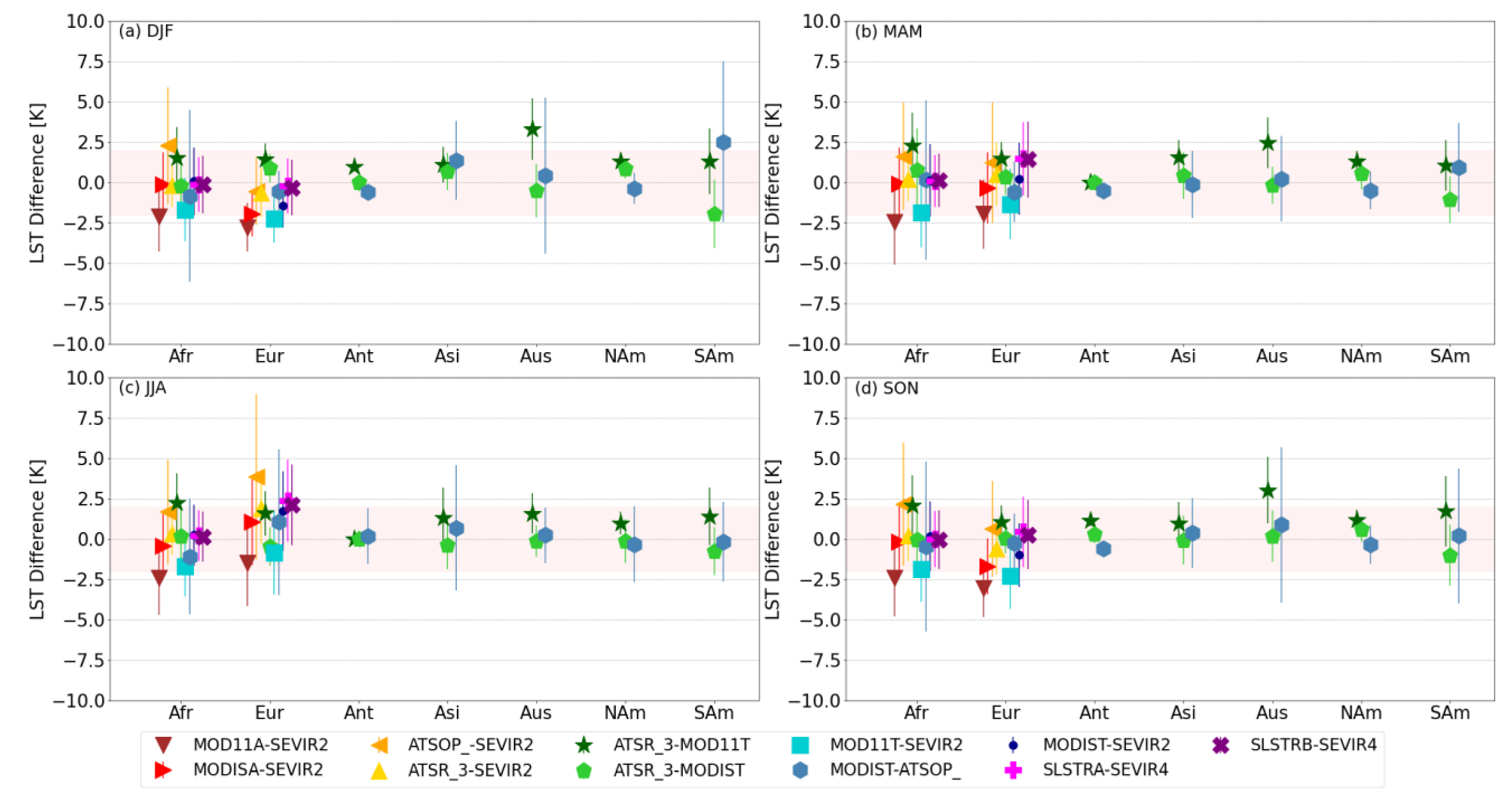
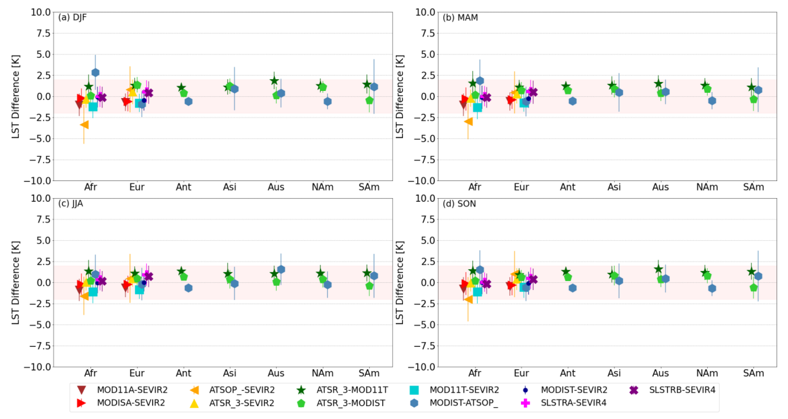
4.1. Continental Intercomparisons Stratified by Seasons

Seasonal median and RSD values of the satellite–satellite differences are shown in Figure 1 for day-time data and in Figure 2 for night-time data. Due to the large averaged areas and the period of 3 years, regional and temporal differences are smoothed out. Thus, these results provide an overview of the seasonal differences at each continent for each satellite data pair. Here, to provide a global overview, polar–polar satellite intercomparisons over continents outside the SEVIRI disk, i.e., Antarctica (Ant), Asia (Asi), Australia (Aus), North America (NAm) and South America (SAm), are shown together with the results for Africa (Afr) and Europe (Eur). The next sections will then focus on the results for Africa and Europe in order to analyse all data sets over a common area, which is limited to SEVIRI’s field of view. Further details about the global analysis will be available in the Product Validation and Intercomparison Report v2 on the LST_cci website (https://climate.esa.int/en/projects/land-surface-temperature/key-documents/, accessed on 14 March 2023).

The higher median differences in day-time data (Figure 1) were observed for ATSR_3–MODIST, which were within 2 K at most continents but reach values of up to 3 K, e.g., over Australia in DJF. Median day-time differences within ±1 K were observed for data pairs formed by LST_cci data sets. Similar differences were found for all data sets at night-time (Figure 2). For most cases, the median differences were within ±1.5 K. For day-time as well as for night-time, ATSR_3–MODIST showed lower differences than ATSR_3-MOD11T and MODIST-ATSOP_ over most continents and for most seasons.

Over Africa and Europe, where all satellite data pairs were intercompared, larger median differences were observed for ATSOP_-SEVIR2, absolute median differences were up to 3.8 K, while MOD11T-SEVIR2 and MOD11A-SEVIR2 showed larger negative differences than the other data pairs. All LST_cci data sets showed a better consistency between them. At night-time, absolute median differences of LST_cci data set comparisons were lower than 0.5 K over Africa and 1.0 K over Europe. For day-time comparisons, absolute median differences of up to 2 K were observed. These differences were larger over Europe, probably caused by differences in the viewing geometry between the polar and geostationary orbit sensors for pixels closer to the SEVIRI disk edge.

The largest RSDs of the differences were observed for MODIST-ATSOP_ and ATSOP_-SEVIR2 satellite data pairs over all continents. However, common RSD between 1 and 2 K were observed for the other combined data sets over all continents, except over Antarctica. In Antarctica, the RSD was lower than 1 K for the three analysed data pairs and for all seasons, except for day-time MODIST-ATSOP_ in JJA, which showed a slightly larger RSD. This is probably due to the lower change of LST with time over ice and the low effect of surface structures in the different viewing geometry of the intercompared satellites.

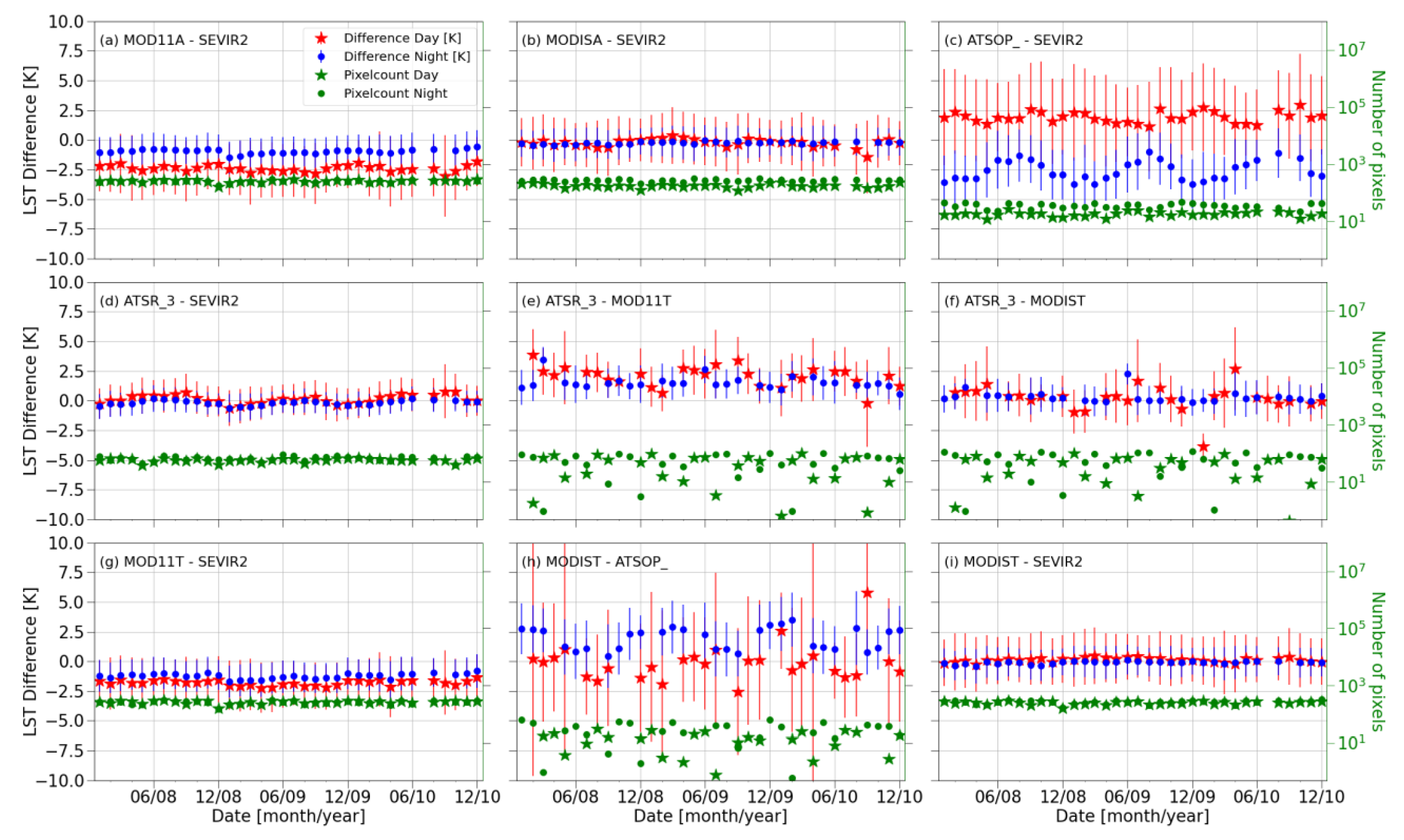
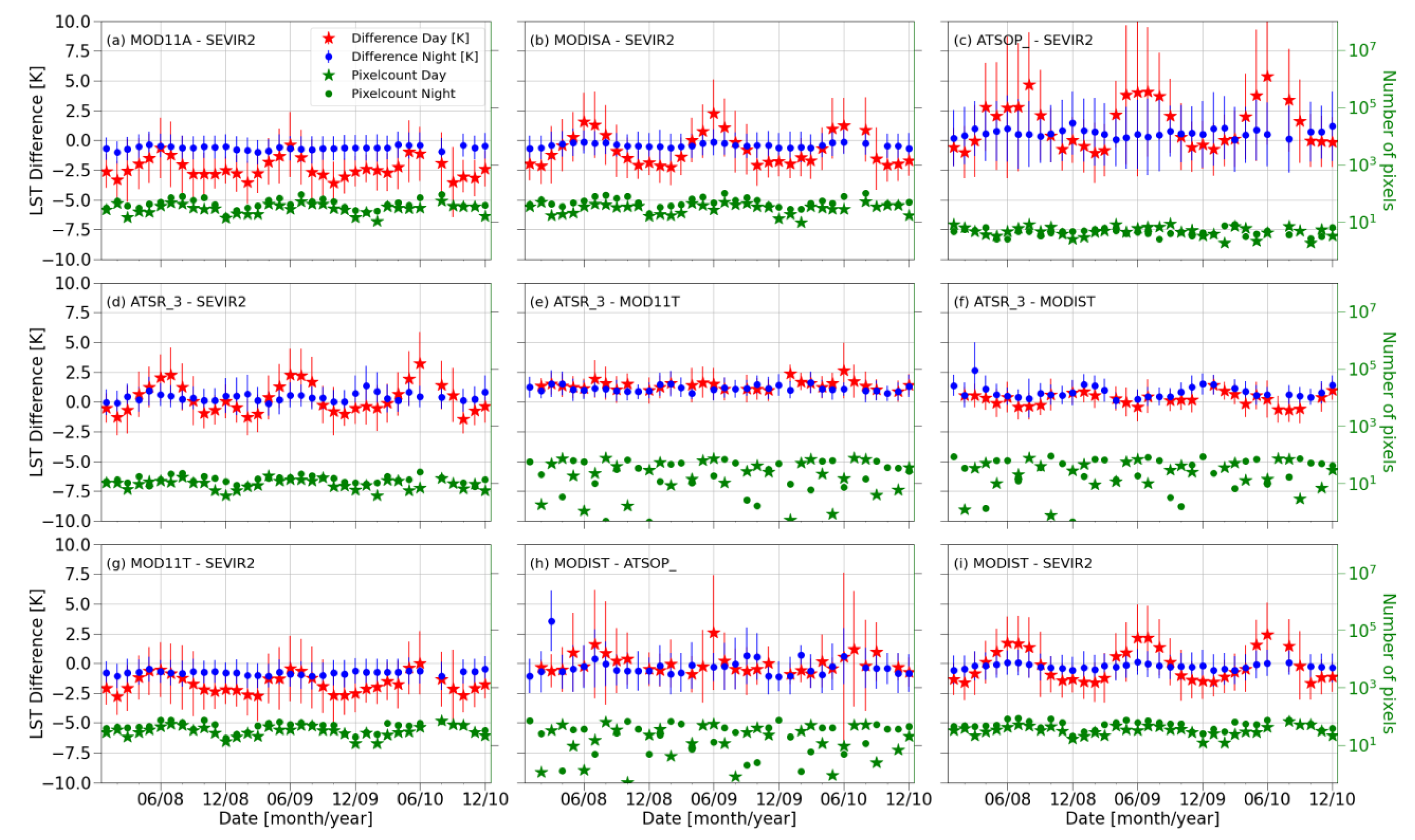
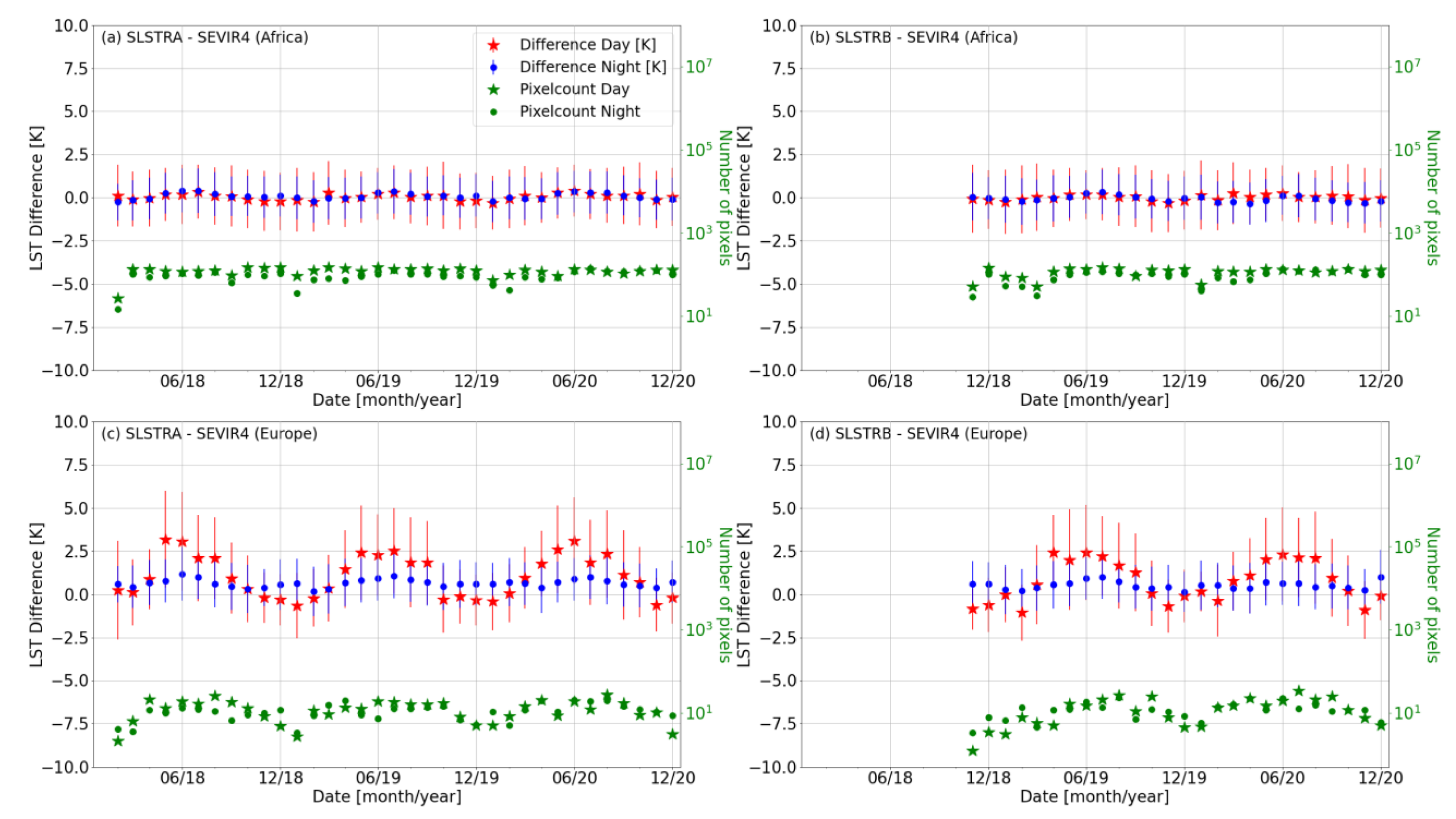
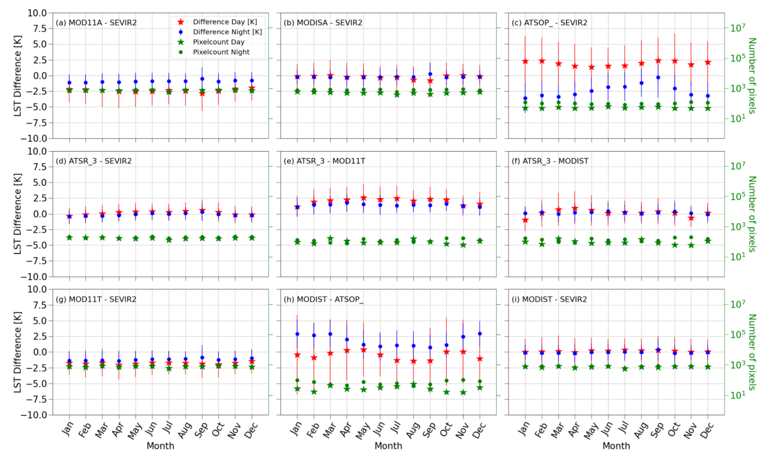
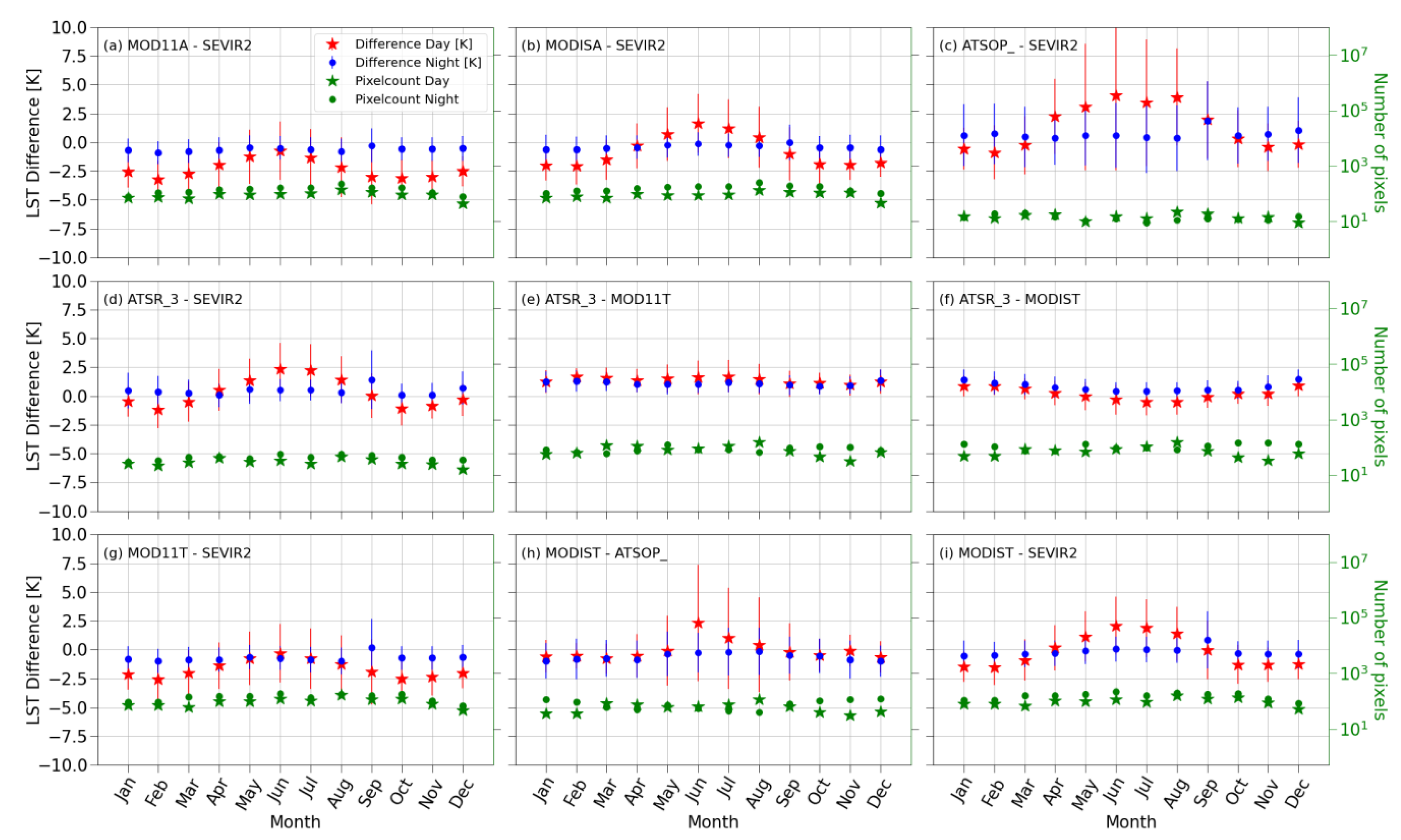
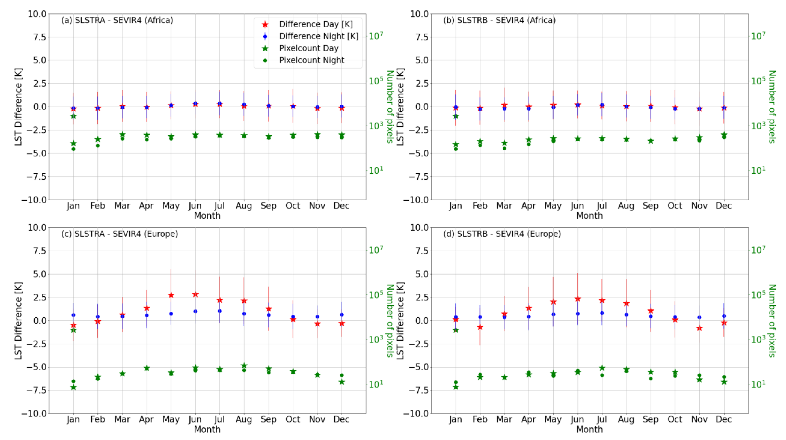
4.2. Monthly Time Series

Monthly median values were analysed over Africa and Europe for the time period covered by each data set, i.e., 2008–2010 for MODISA/T, ATSR_3, ATSOP_ and SEVIR2 data sets and 2018–2020 for SLSTRA/B and SEVIR4 data sets. Figure 3 and Figure 4 show the median of differences for the data pairs analysed in 2008–2010 over Africa and Europe, respectively, and the corresponding RSD represented as error bars. Figure 5 shows the monthly time series for the intercompared satellite data sets in 2018–2020. Day-time intercomparisons showed median differences between −3.9 and 5.4 K and RSD between 0.6 and 7.1 K. At night-time, median of differences between −3.8 and 4.7 K and RSD between 0.5 and 3.2 K were observed. The larger RSDs were observed for the ATSOP_-SEVIR2 data pair.

Results in Figure 3 and Figure 4 show that the satellite data pair ATSOP_-SEVIR2 had the largest absolute median difference over Africa and Europe, followed by MODIST-ATSOP_. The intercomparisons between the operational and LST_cci MODIS data sets and SEVIR2 gave the highest number of datapoints. MOD11A-SEVIR2 and MOD11T-SEVIR2 showed larger negative differences compared to the MODIST-SEVIR2 and MODISA-SEVIR2 data sets over Africa and Europe, and larger RSDs at day-time for the latter. The MODIS LST_cci data sets covered differences with SEVIR2 within ±2.5 K, while MODISA-SEVIR2 and MODIST-SEVIR2 differences ranged from −3 to 0 K. Differences for ATSR_3-SEVIR2 were lower than those observed for ATSR_3-MODIST and ATSR_3-MOD11T over Africa. However, these results were reversed over Europe, where the comparison of ATSR_3 against SEVIR2 showed higher differences than both MODIS data sets. Regarding the intercomparison of SLSTRA and SLSTRB with SEVIR4 (Figure 5), small differences were observed over Africa, but positive median differences with a clear seasonality were observed over Europe for both data sets. To better distinguish seasonal characteristics in the intercompared data sets, Figure 6, Figure 7 and Figure 8 show the monthly aggregated median differences for all available intercomparisons in 2008–2010 over Africa (Figure 6) and Europe (Figure 7) and for the period 2018–2020 for SLSTR-A/B (Figure 8).

No clear seasonal variation was observed over Africa (Figure 6) except for ATSOP_-SEVIR2 and MODIST-ATSOP_, probably due to the high number of pixels between the tropics, where seasonalities are not as pronounced as for medium and high latitudes. However, all data sets compared against SEVIR2 and SEVIR4 over Europe showed a seasonal cycle of the median differences, with an annual amplitude up to 4.5 K (e.g., Figure 7b), as well as of the number of datapoints (Figure 4 and Figure 5). For the LST_cci data sets (Figure 7b,d,f,h,i and Figure 8c,d), the monthly median differences were around 0 K, with positive differences in summer and negative in winter.

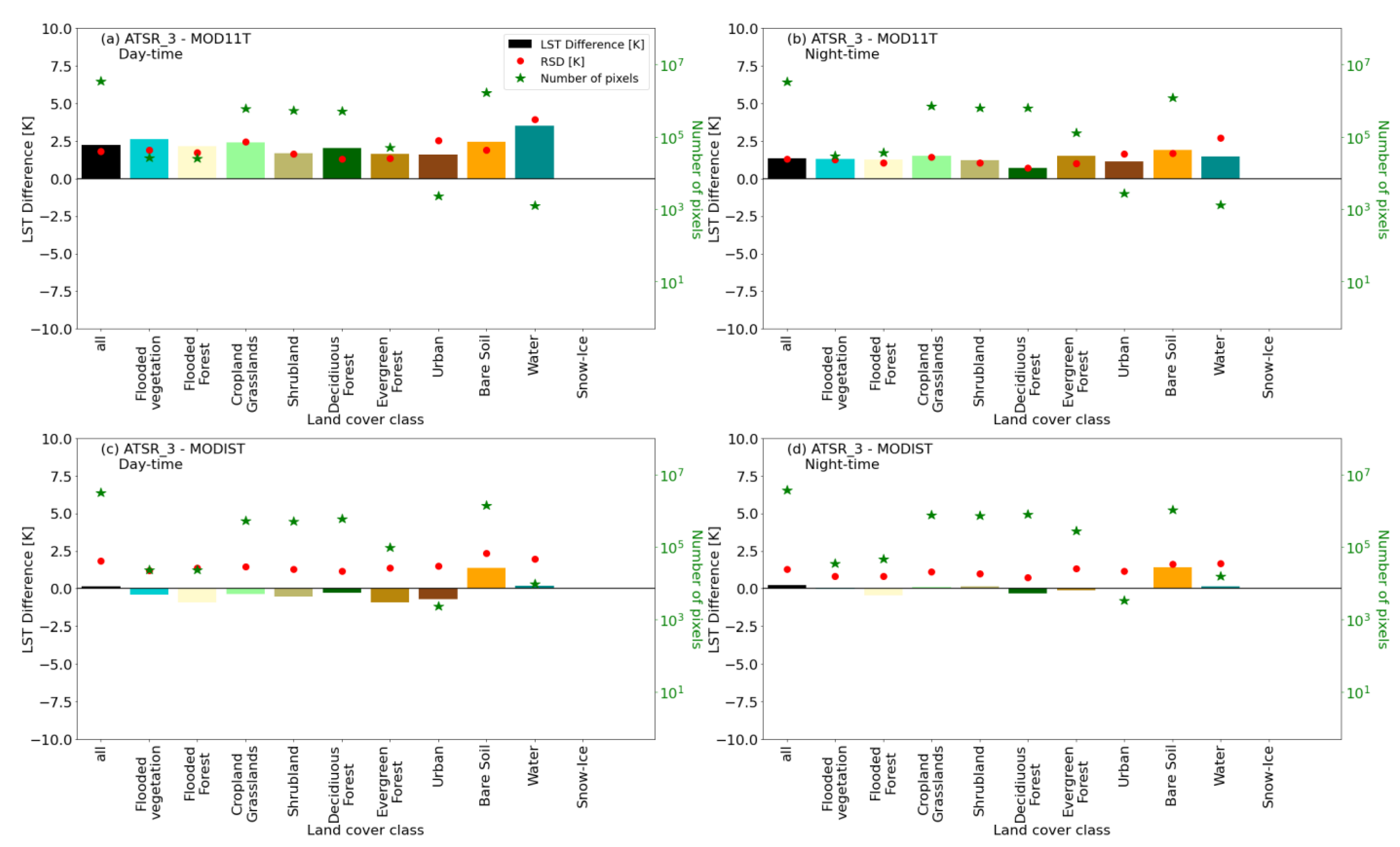
4.3. Land Cover Analysis

The satellite data pairs were analysed according to the pixel’s land cover class (Table 2). Figure 9 and Figure 10 show seasonal median differences and RSD for NASA’s operational and LST_cci MODIS data sets intercompared with SEVIR2 (Figure 9) and ATSR_3 (Figure 10) for each land cover class. These data pairs were selected as representative examples of intercomparisons between polar–geostationary orbit sensors and polar–polar orbit sensors. Additionally, the number of datapoints for each land cover class is shown. The most frequent land cover class over Africa was bare soil. Over Europe, the most frequent class was the generic cropland and grassland class.

Differences for winter and summer day-time MODIST-SEVIR2 and MOD11T-SEVIR2 data pairs over Europe are shown in Figure 9. Negative median differences were observed in winter (DJF) for both MODIST-SEVIR2 and MOD11T-SEVIR2. However, in summer the LST_cci data set showed positive differences (Figure 9b), while NASA’s operational data set yielded negative differences over most land cover classes (Figure 9d). Larger differences were observed over bare soils for MOD11T-SEVIR2 in winter and MODIST-SEVIR2 in summer, but also the corresponding RSD was larger than for most land covers, i.e., only water and snow-ice land covers showed larger RSDs. For example, in summer, the RSD for MOD11T-SEVIR2 (Figure 9b) showed values up to 5 K. Although low median values were found for summer in the MOD11T-SEVIR2 data set (except for the snow-ice class), the corresponding RSDs were larger than for the other data sets, with RSD values larger than 2.5 K for most land covers. For both intercompared data sets, summer RSDs are larger than winter RSDs, which is probably related to a higher impact of viewing geometry differences in summer, when the temperature differences between sunlit and shaded areas are larger. In winter, slightly larger RSDs were observed for the shrubland class, but similar to those observed over forests and urban areas. Similar results were obtained over Africa: as for MODIST-SEVIR2, in summer for ATSOP_-SEVIR2 (not shown), positive differences were observed, while they were negative in winter for most land covers. For night-time data, all data sets provided lower differences than for day-time. Regarding SLSTRA/B-SEVIR4 data sets (not shown), larger differences than those observed for the other data sets were found, which were extremely large in some cases at day-time, up to 10 K, but lower (around 2.5 K) for night-time data.

Night-time and day-time median differences of ATSR_3-MODIST and ATSR_3-MOD11T data sets are shown in Figure 10 for each land cover and summer season as a representative example of polar–polar orbit satellite data pair. Positive differences were observed for all land cover classes in the ATSR_3-MOD11T data set, which were larger at day-time with median differences of up to 3 K, while they were around 1 K for night-time data. However, ATSR_3 showed good agreement with MODIST for day-time and night-time, with differences of around 0 K for all land cover classes except for bare soils. For the latter, positive differences were found at day-time and night-time with similar differences below 2 K, although the RSDs were slightly larger at day-time (day-time RSD of 2.5 K and night-time of RSD of 2 K). Regarding the RSD, for most land cover classes, similar values between 2 and 2.5 K were observed for the ATSR_3-MOD11T day-time data set. While RSDs around 1.5 K were observed for night-time intercomparisons.

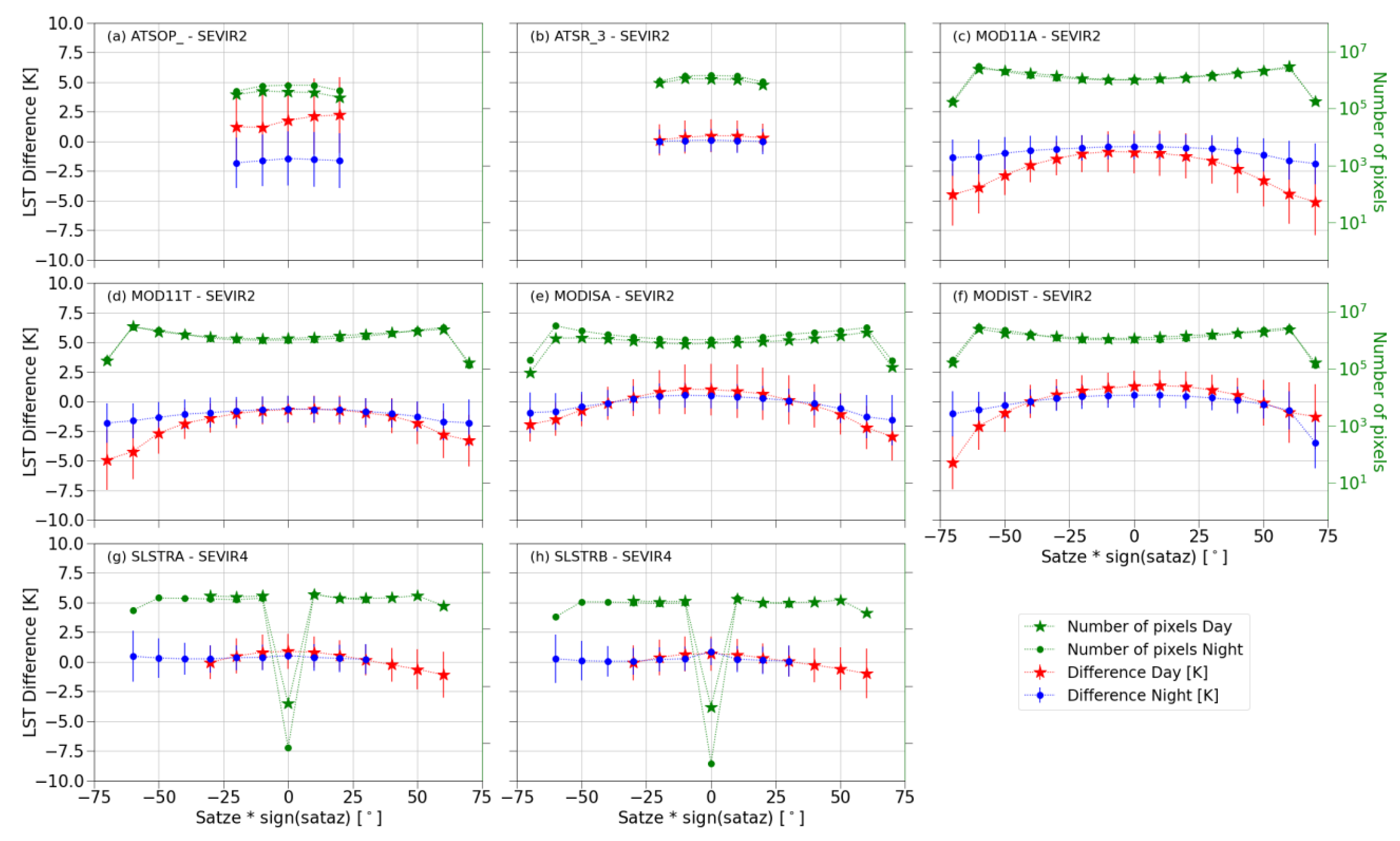
4.4. Intercomparison Analysis Considering the Viewing Geometry

Similar results were observed over Europe and Africa when comparing the median differences with the viewing geometry for each satellite–satellite data pair. Since no significant seasonal variation was found for the different viewing geometries, for each combination of polar–geostationary orbit satellite data pair over Africa, only summer median differences stratified by viewing geometry are shown in Figure 11. For day-time and night-time data, the number of datapoints in each viewing geometry bin is also shown. For ATSOP_ and ATSR_3 data sets, no data were found for zenith viewing angles larger than 22°, which is due to the narrow field of view of AATSR. Similarly, because of the asymmetric swath of SLSTR, only satze*sign(sataz) between −35° and 60° were found for the day-time data and between −60° and 35° for the night-time data. For the viewing zenith angles ranging from −10° to 10°, the number of SLSTRA/B-SEVIR4 datapoints was considerably lower than for larger viewing zenith angles. The number of MODIS datapoints increased symmetrically with viewing zenith angle except for bins at ±65°, because these two bins exceed the swath of MODIS.

No significant variation with viewing zenith angle was observed for the ATSR_R-SEVIR2 and ATSOP_-SEVIR2 data sets because of the small range of viewing angles. However, an asymmetric variation of the differences for day-time data was observed for the four MODIS data sets. The differences increase from nadir to large negative values. In the case of MODIST and MOD11T data sets, these differences became larger for negative sataz values, but for MODISA and MOD11A, larger for positive sataz values. This is related to the local overpass time of the MODIS sensors; since the descending orbit (day-time) MODIS-TERRA overpass is in the morning, it observes more shadowy than sunlit areas when looking from west to east, i.e., for negative sataz. In contrast, the daily MODISA overpass occurs in the early afternoon and therefore more shadow areas are seen for the east to west satellite view, i.e., at positive sataz. At night-time, when LST is not affected by solar irradiance and thermal homogeneity is higher, the decrease in median differences is symmetric for all data sets and smaller than at day-time. SLSTRA-SEVIR4 and SLSTRB-SEVIR4 showed no significant variation with zenith angle for the night-time data, but a slight decrease of median differences for zenith angles larger than 40° at day-time.

5. Conclusions

Ten LST products (i.e., ATSR_3, MODISA, MODIST, SLSTRA, SLSTRB, SEVIR2, SEVIR4, MOD11A, MOD11T and ATSOP_) were intercompared in eleven different combinations of satellite–satellite data pairs: eight polar–geostationary orbit satellite data sets and three polar–polar orbit satellite data sets. Each data set was analysed and investigated for monthly and seasonal median differences over Europe and Africa. A larger median difference was observed for ATSOP_-SEVIR2 over Europe in winter and over Africa in summer. Additionally, the three polar–polar orbit satellite data sets were investigated over all continents, yielding similar results over most of them. Overall, the satellite data pairs comparing two LST_cci data sets agreed better with each other (median differences < 2 K) than pairs involving an LST operational product, i.e., NASA operational MODIS LST product (MOD11A and MOD11T) or ESA’s AATSR LST product (ATSOP_).

For day-time data over Europe, a significant seasonality was observed in the intercomparisons of monthly averaged differences between polar and geostationary orbit sensors (i.e., SEVIR2 and SEVIR4 data); in contrast, no seasonality was observed for day-time data over Africa. This could be caused by differences in sensor viewing geometries for polar and geostationary satellites, e.g., Europe is mainly represented by pixels near the edge of the SEVIRI disk. Pairs of night-time LST_cci data sets over Europe and Africa data showed good agreement, while the operational products generally underestimated about 1 K SEVIR2 LST. A similar underestimation of about 2 K was also observed for day-time data and indicates that there is a bias between NASA’s operational MODIS LST product and the LST_CCI MODIS data sets. These results agree with those in [36], who found that MODIS MOD11 and MYD11 LST products underestimated in situ data at most of the investigated sites. In Ref. [36], the authors reported mean biases of −2.1 K and −0.7 K for day-time and night-time data, respectively, which are similar to the differences between the operational MODIS LSTs and SEVIR2 data determined in this study.

Additionally, the median differences obtained for each satellite–satellite data pair were analysed stratified by land cover class and satellite viewing geometry. For both continents, the analysis revealed a lower agreement between data sets over bare soil areas. However, no significant differences in bias or RSD were observed between vegetated land cover classes, e.g., cropland and grasslands, shrubland, evergreen forest and deciduous forest. Furthermore, no land cover class showed a clear seasonality of median differences, although the performance of some satellite data pairs depended on the season, e.g., in winter, MODIST-SEVIR2 day-time data over Europe showed negative differences for all land cover classes but positive ones in summer. Overall, when considering all land covers, the best agreement was observed for the ATSR_3-MODIST data set, both at day-time and night-time; only some pixels classified as bare soil showed larger discrepancies.

Furthermore, for large zenith angles in the intercomparison between MODIS and SEVIR2, an increase of absolute median differences was observed. This increase was symmetric for night-time data and is probably related to differences between the field of view of the two sensors but also to differences in their view angles, which results in differences in observed canopy fractions, as well as in an emissivity anisotropy over arid areas [37]. Since a large extent of its observed Earth disk is desert, emissivity anisotropy is particularly relevant for SEVIRI. Furthermore, the observed dependencies of night-time biases on view angle agree with results reported in [38] for night-time LST from the Advanced Very High-Resolution Radiometer (AVHRR) and SEVIRI LST. In contrast, at day-time, the differences were considerably larger and asymmetric with respect to nadir; this suggests that these differences are linked to illumination geometry and reflect the viewing geometry dependence of shadow and sunlit areas in the sensor’s field of view. As a consequence, the observed negative differences were larger for negative azimuthal viewing angles of MODIS-TERRA, but they were larger for positive azimuthal viewing angles of MODIS-AQUA.

Overall, despite their retrieval with different split-window algorithms, all LST_CCI data sets had a good correlation between them. Although the intercomparisons of the LST_CCI data sets with SEVIR2 and SEVIR4 data showed better agreement than the corresponding intercomparisons for the operational LST data products, in most cases, the intercomparisons yielded median differences of less than 2 K, which is the uncertainty associated with the LST_cci SEVIR2 and SEVIR4 products.

References

1. GCOS. The 2022 GCOS ECVs Requirements (GCOS 245); World Meteorological Organization: Geneva, Switzerland, 2022. [Google Scholar]
2. GCOS. The Global Observing System for Climate: Implementation Needs; World Meteorological Organization: Geneva, Switzerland, 2016; Volume 200, p. 341. [Google Scholar]
3. Hollmann, R.; Merchant, C.J.; Saunders, R.; Downy, C.; Buchwitz, M.; Cazenave, A.; Chuvieco, E.; Defourny, P.; De Leeuw, G.; Forsberg, R.; et al. The ESA Climate Change Initiative: Satellite Data Records for Essential Climate Variables. Bull. Am. Meteorol. Soc. 2013, 94, 1541–1552. [Google Scholar] [CrossRef] [Green Version]
4. Plummer, S.; Lecomte, P.; Doherty, M. The ESA Climate Change Initiative (CCI): A European Contribution to the Generation of the Global Climate Observing System. Remote Sens. Environ. 2017, 203, 2–8. [Google Scholar] [CrossRef]
5. Perry, M.; Ghent, D.J.; Jiménez, C.; Dodd, E.M.A.; Ermida, S.L.; Trigo, I.F.; Veal, K.L. Multisensor Thermal Infrared and Microwave Land Surface Temperature Algorithm Intercomparison. Remote Sens. 2020, 12, 4164. [Google Scholar] [CrossRef]
6. Cheval, S.; Dumitrescu, A.; Amihăesei, V.; Irașoc, A.; Paraschiv, M.G.; Ghent, D. A Country Scale Assessment of the Heat Hazard-Risk in Urban Areas. Build. Environ. 2023, 229, 109892. [Google Scholar] [CrossRef]
7. Cheval, S.; Dumitrescu, A.; Irașoc, A.; Paraschiv, M.G.; Perry, M.; Ghent, D. MODIS-Based Climatology of the Surface Urban Heat Island at Country Scale (Romania). Urban Clim. 2022, 41, 101056. [Google Scholar] [CrossRef]
8. Sismanidis, P.; Bechtel, B.; Perry, M.; Ghent, D. The Seasonality of Surface Urban Heat Islands across Climates. Remote Sens. 2022, 14, 2318. [Google Scholar] [CrossRef]
9. Karagali, I.; Barfod Suhr, M.; Mottram, R.; Nielsen-Englyst, P.; Dybkjær, G.; Ghent, D.; Høyer, J.L. A New Level 4 Multi-Sensor Ice Surface Temperature Product for the Greenland Ice Sheet. Cryosphere 2022, 16, 3703–3721. [Google Scholar] [CrossRef]
10. Good, E.J.; Aldred, F.M.; Ghent, D.J.; Veal, K.L.; Jimenez, C. An Analysis of the Stability and Trends in the LST_cci Land Surface Temperature Datasets Over Europe. Earth Space Sci. 2022, 9, e2022EA002317. [Google Scholar] [CrossRef]
11. Mallick, K.; Baldocchi, D.; Jarvis, A.; Hu, T.; Trebs, I.; Sulis, M.; Bhattarai, N.; Bossung, C.; Eid, Y.; Cleverly, J.; et al. Insights Into the Aerodynamic Versus Radiometric Surface Temperature Debate in Thermal-Based Evaporation Modeling. Geophys. Res. Lett. 2022, 49, e2021GL097568. [Google Scholar] [CrossRef]
12. Guillevic, P.; Göttsche, F.; Nickeson, J.; Hulley, G.; Ghent, D.; Yu, Y.; Trigo, I.; Hook, S.; Sobrino, J.A.; Remedios, J.; et al. Land Surface Temperature Product Validation Best Practice Protocol. Version 1.1. In Best Practice for Satellite-Derived Land Product Validation; Land Product Validation Subgroup (WGCV/CEOS): London, UK, 2018; p. 58. [Google Scholar] [CrossRef]
13. Göttsche, F.M.; Olesen, F.S.; Trigo, I.F.; Bork-Unkelbach, A.; Martin, M.A. Long Term Validation of Land Surface Temperature Retrieved from MSG/SEVIRI with Continuous in-Situ Measurements in Africa. Remote Sens. 2016, 8, 410. [Google Scholar] [CrossRef] [Green Version]
14. Martin, M.A.; Ghent, D.; Pires, A.C.; Göttsche, F.M.; Cermak, J.; Remedios, J.J. Comprehensive in Situ Validation of Five Satellite Land Surface Temperature Data Sets over Multiple Stations and Years. Remote Sens. 2019, 11, 479. [Google Scholar] [CrossRef] [Green Version]
15. Pérez-Planells, L.; Niclòs, R.; Puchades, J.; Coll, C.; Göttsche, F.M.; Valiente, J.A.; Valor, E.; Galve, J.M. Validation of Sentinel-3 Slstr Land Surface Temperature Retrieved by the Operational Product and Comparison with Explicitly Emissivity-Dependent Algorithms. Remote Sens. 2021, 13, 2228. [Google Scholar] [CrossRef]
16. Ghent, D.; Corlett, G.K.; Göttsche, F.M.; Remedios, J.J. Global Land Surface Temperature From the Along-Track Scanning Radiometers. J. Geophys. Res. Atmos. 2017, 122, 12167–12193. [Google Scholar] [CrossRef] [Green Version]
17. Martins, J.P.A.; Trigo, I.F.; Ghilain, N.; Jimenez, C.; Göttsche, F.-M.; Ermida, S.L.; Olesen, F.-S.; Gellens-Meulenberghs, F.; Arboleda, A. An All-Weather Land Surface Temperature Product Based on MSG/SEVIRI Observations. Remote Sens. 2019, 11, 3044. [Google Scholar] [CrossRef] [Green Version]
18. Coll, C.; Wan, Z.; Galve, J.M. Temperature-Based and Radiance-Based Validations of the V5 MODIS Land Surface Temperature Product. J. Geophys. Res. Atmos. 2009, 114, 1–15. [Google Scholar] [CrossRef] [Green Version]
19. Wan, Z. New Refinements and Validation of the Collection-6 MODIS Land-Surface Temperature/Emissivity Product. Remote Sens. Environ. 2014, 140, 36–45. [Google Scholar] [CrossRef]
20. Perez-Planells, L.; Niclos, R.; Valor, E.; Gottsche, F.-M. Retrieval of Land Surface Emissivities Over Partially Vegetated Surfaces From Satellite Data Using Radiative Transfer Models. IEEE Trans. Geosci. Remote Sens. 2022, 60, 1–21. [Google Scholar] [CrossRef]
21. Hook, S.J.; Vaughan, R.G.; Tonooka, H.; Schladow, S.G. Absolute Radiometric In-Flight Validation of Mid Infrared and Thermal Infrared Data From ASTER and MODIS on the Terra Spacecraft Using the Lake Tahoe, CA/NV, USA, Automated Validation Site. IEEE Trans. Geosci. Remote Sens. 2007, 45, 1798–1807. [Google Scholar] [CrossRef]
22. Hook, S.J.; Cawse-Nicholson, K.; Barsi, J.; Radocinski, R.; Hulley, G.C.; Johnson, W.R.; Rivera, G.; Markham, B. In-Flight Validation of the ECOSTRESS, Landsats 7 and 8 Thermal Infrared Spectral Channels Using the Lake Tahoe CA/NV and Salton Sea CA Automated Validation Sites. IEEE Trans. Geosci. Remote Sens. 2020, 58, 1294–1302. [Google Scholar] [CrossRef]
23. Merchant, C.J.; Matthiesen, S.; Rayner, N.A.; Remedios, J.J.; Jones, P.D.; Olesen, F.; Trewin, B.; Thorne, P.W.; Auchmann, R.; Corlett, G.K.; et al. The Surface Temperatures of Earth: Steps towards Integrated Understanding of Variability and Change. Geosci. Instrum. Methods Data Syst. 2013, 2, 305–321. [Google Scholar] [CrossRef] [Green Version]
24. Martin, M. CCI Land. Surface Temperature Product. Validation and Intercomparison Report (PVIR). 2020. Available online: https://admin.climate.esa.int/media/documents/LST-CCI-D4.1-PVIR_-_i1r0_-_Product_Validation_and_Intercomparison_Report.pdf (accessed on 26 June 2022).
25. Wan, Z.; Dozier, J. A Generalized Split-Window Algorithm for Retrieving Land-Surface Temperature from Space. IEEE Trans. Geosci. Remote Sens. 1996, 34, 892–905. [Google Scholar] [CrossRef] [Green Version]
26. Prata, F. Land Surface Temperature Measurement from Space: AATSR Algorithm Theoretical Basis Document. In Contract Report to ESA; CSIRO Atmospheric Research: Aspendale, VIC, Australia, 2002; Volume 2002, pp. 1–34. [Google Scholar]
27. Kirches, G.; Brockman, C.; Boettcher, M.; Peters, M.; Bontemps, S.; Lamarche, C.; Schlerf, M.; Santoro, M.; Defourny, P. Land Cover CCI Product User Guide; Version 2. 2017. Available online: https://maps.elie.ucl.ac.be/CCI/viewer/download/ESACCI-LC-Ph2-PUGv2_2.0 (accessed on 26 June 2022).
28. Hersbach, H.; Bell, B.; Berrisford, P.; Hirahara, S.; Horányi, A.; Muñoz-Sabater, J.; Nicolas, J.; Peubey, C.; Radu, R.; Schepers, D.; et al. The ERA5 Global Reanalysis. Q. J. R. Meteorol. Soc. 2020, 146, 1999–2049. [Google Scholar] [CrossRef]
29. Ghent, D.; Veal, K.; Trent, T.; Dodd, E.; Sembhi, H.; Remedios, J. A New Approach to Defining Uncertainties for MODIS Land Surface Temperature. Remote Sens. 2019, 11, 1021. [Google Scholar] [CrossRef] [Green Version]
30. Borbas, E.; Hulley, G.; Feltz, M.; Knuteson, R.; Hook, S. The Combined ASTER MODIS Emissivity over Land (CAMEL) Part 1: Methodology and High Spectral Resolution Application. Remote Sens. 2018, 10, 643. [Google Scholar] [CrossRef] [Green Version]
31. Ghent, D.; Dodd, E.; Veal, U.K.; Perry, M.; Carlos, U.; Estellus, J.; Ermida, S. CCI Land. Surface Temperature Algorithm Theoretical Basis Document; Institute for Computational Earth System Science: Santa Barbara, CA, USA, 2021. [Google Scholar]
32. Bicheron, P.; Defourny, P.; Brockmann, C.; Schouten, L.; Vancutsem, C.; Huc, M.; Bontemps, S.; Leroy, M.; Achard, F.; Herold, M.; et al. GLOBCOVER 2009 Products Description and Validation Report; Medias France: Paris, France, 2011; Volume 136. [Google Scholar]
33. Caselles, E.; Valor, E.; Abad, F.; Caselles, V. Automatic classification-based generation of thermal infrared land surface emissivity maps using AATSR data over Europe. Remote Sens. Environ. 2012, 124, 321–333. [Google Scholar] [CrossRef] [Green Version]
34. Goldberg, M.; Ohring, G.; Butler, J.; Cao, C.; Datla, R.; Doelling, D.; Gärtner, V.; Hewison, T.; Iacovazzi, B.; Kim, D.; et al. The Global Space-Based Inter-Calibration System. Bull. Am. Meteorol. Soc. 2011, 92, 467–475. [Google Scholar] [CrossRef]
35. Wilrich, P.T. Robust Estimates of the Theoretical Standard Deviation to Be Used in Interlaboratory Precision Experiments. Accredit. Qual. Assur. 2007, 12, 231–240. [Google Scholar] [CrossRef]
36. Duan, S.-B.; Li, Z.-L.; Li, H.; Göttsche, F.-M.; Wu, H.; Zhao, W.; Leng, P.; Zhang, X.; Coll, C. Validation of Collection 6 MODIS Land Surface Temperature Product Using in Situ Measurements. Remote Sens. Environ. 2019, 225, 16–29. [Google Scholar] [CrossRef] [Green Version]
37. Ermida, S.L.; Trigo, I.F.; Hulley, G.; DaCamara, C.C. A Multi-Sensor Approach to Retrieve Emissivity Angular Dependence over Desert Regions. Remote Sens. Environ. 2020, 237, 111559. [Google Scholar] [CrossRef]
38. Trigo, I.F.; Ermida, S.L.; Martins, J.P.A.; Gouveia, C.M.; Göttsche, F.-M.; Freitas, S.C. Validation and Consistency Assessment of Land Surface Temperature from Geostationary and Polar Orbit Platforms: SEVIRI/MSG and AVHRR/Metop. ISPRS J. Photogramm. Remote Sens. 2021, 175, 282–297. [Google Scholar] [CrossRef]
Figure 1. Seasonal day-time median differences over each continent for all satellite–satellite data pairs. The error bar is the RSD of the differences for each satellites data pair. The coloured area indicates the range of median differences within ±2 K.
Remotesensing 15 03281 g001
Figure 2. Seasonal night-time median differences over each continent for all satellite–satellite data pairs. The error bar is the RSD of the differences for each satellite data pair. The coloured area indicates the range of median differences within ±2 K.
Remotesensing 15 03281 g002
Figure 3. Day-time (red stars) and night-time (blue dots) monthly median differences and RSD for all satellite–satellite intercomparisons in the period 2008–2010 over Africa. The number of averaged pixels (green stars) is given on the right axis.
Remotesensing 15 03281 g003
Figure 4. Day-time (red stars) and night-time (blue dots) monthly median differences and RSD for all satellite–satellite intercomparisons in the period 2008–2010 over Europe. The number of averaged pixels (green stars) is given on the right axis.
Remotesensing 15 03281 g004
Figure 5. Day-time (red stars) and night-time (blue dots) monthly median differences and RSD for SLSTRA/B-SEVIR4 intercomparisons in the period 2018–2020 over Africa (a,b) and Europe (c,d). The number of averaged pixels (green stars) is given on the right axis.
Remotesensing 15 03281 g005
Figure 6. Day-time (red stars) and night-time (blue dots) monthly aggregated median differences and RSD for all satellite–satellite intercomparisons in the period 2008–2010 over Africa.
Remotesensing 15 03281 g006
Figure 7. Day-time (red stars) and night-time (blue dots) monthly aggregated median differences and RSD for all satellite–satellite intercomparisons in the period 2008–2010 over Europe.
Remotesensing 15 03281 g007
Figure 8. Day-time (red stars) and night-time (blue dots) monthly aggregated median differences and RSD for SLSTRA/B-SEVIR4 intercomparisons in the period 2018–2020 over Africa (a,b) and Europe (c,d).
Remotesensing 15 03281 g008
Figure 9. Winter ‘DJF’ and Summer ‘JJA’ day-time differences of MODIST-SEVIR2 and MOD11T-SEVIR2 data sets for each generic LCC (Table 2) over Europe. The differences are shown for: (a) MODIST-SEVIR2 DJF, (b) MODIST-SEVIR2 JJA, (c) MOD11T-SEVIR2 DJF and (d) MOD11T-SEVIR2 JJA.
Remotesensing 15 03281 g009
Figure 10. Summer (JJA) differences of ATSR_3-MOD11T and ATSR_3-MODIST data sets for each generic LCC (Table 2) over Africa. The differences are shown for: (a) ATSR_3-MOD11T day-time, (b) ATSR_3-MOD11T night-time, (c) ATSR_3-MODIST day-time and (d) ATSR_3-MODIST night-time.
Remotesensing 15 03281 g010
Figure 11. Summer median differences against the polar viewing geometry for the polar–geostationary orbit satellite data pairs over Africa: (a) ATSOP_-SEVIR2, (b) ATSR_3-SEVIR2, (c) MOD11A-SEVIR2, (d) MOD11T-SEVIR2, (e) MODISA-SEVIR2, (f) MODIST-SEVIR2, (g) SLSTRA-SEVIR4 and (h) SLSTRB-SEVIR4.
Remotesensing 15 03281 g011