Abstract
The visual object tracking technology of remote sensing images has important applications in areas with high safety performance such as national defense, homeland security, and intelligent transportation in smart cities. However, previous research demonstrates that adversarial examples pose a significant threat to remote sensing imagery. This article first explores the impact of adversarial examples in the field of visual object tracking in remote sensing imagery. We design a classification- and regression-based loss function for the popular Siamese RPN series of visual object tracking models and use the PGD gradient-based attack method to generate adversarial examples. Additionally, we consider the temporal consistency of video frames and design an adversarial examples attack method based on momentum continuation. We evaluate our method on the remote sensing visual object tracking datasets SatSOT and VISO and the traditional datasets OTB100 and UAV123. The experimental results show that our approach can effectively reduce the performance of the tracker.
1. Introduction
Visual object tracking (VOT) refers to the process of finding a target to be tracked in the first frame of a video, with the aim of accurately locating the target’s position in subsequent frames and precisely outlining it with anchor box. Compared to traditional VOT methods, satellite video object tracking benefits from a wider shooting range, often resulting in higher efficiency in monitoring targets in applications such as military reconnaissance [1,2,3], traffic monitoring [4,5,6], and wildlife tracking [7,8,9].
The success of visual object tracking heavily relies on the features of the template, and deep learning networks have been remarkably successful in feature extraction. As a result, deep learning network models have become a major focus of research in VOT. Remote sensing image (RSI) visual tracking can be divided into two categories: offline tracking and online tracking. Online tracking methods can be further divided into correlation-filter-based methods, tracking by detection, deep-learning-based models, and optical-flow-based methods. Neural network models are typically designed to be end-to-end, meaning that the entire model’s input and output are observable, and the model performs all necessary computations during the end-to-end process. This design simplifies the entire system, and the neural network can automatically learn these steps, accelerating the development process. However, the end-to-end design turns deep-learning-based models into “black boxes”, and Szegedy et al. [10] were the first to discover the existence of adversarial examples in natural datasets, which can render a trained classifier model ineffective. The researchers in [11] proposed the backdoor attack on the VOT task, so the deep neural network model also suffers from various security problems.
When deploying deep learning models in the real world, it is important to consider their robustness and their ability to resist interference from malicious input data. Adversarial examples occur during the testing phase and involve the addition of carefully crafted perturbations to input samples. These perturbations are designed to be imperceptible to the human eye but have the ability to render deep neural network models ineffective. There are currently two methods for generating adversarial examples. The first is gradient-based methods, such as L-BFGS [12], FGSM [13], and PGD [14], which use the gradient information of the model to generate adversarial examples. During the neural network training phase, the loss function is minimized through the gradient descent algorithm to achieve optimal network weight parameters. The gradient-based method can iteratively perturb the input data by quickly calculating the model’s gradient information. The second method is optimization-based methods, such as C&W [15], which minimize a loss function to find an adversarial example that is similar to the original sample, while causing the model to misclassify it. These algorithms are mainly focused on natural images, but Czaja et al. [16] were the first to reveal the existence of adversarial examples in the remote sensing field.
Adversarial examples research is essential in designing secure and reliable deep neural network models for remote sensing images, especially in military contexts. Currently, there have been studies on adversarial examples in remote sensing image (RSI) classification [17,18,19,20] and detection [21,22,23]. The authors of Ref. [24] proposed the first method for generating adversarial examples in RSI. Several basic CNN models widely used in RSI recognition systems were trained, and various attack algorithms were used to generate different adversarial examples. The experimental results have demonstrated that adversarial examples indeed pose a significant threat to high-accuracy CNN models in RSI (Remote Sensing Imagery) recognition. Furthermore, the similarity between the adversarial example and the corresponding class significantly influences the success of the attack. The authors of Ref. [25] investigated the FGSM and BIM [26]. The authors of Ref. [27] attacked CNN-based RSI classification models, such as InceptionV1 [28], ResNet [29], and AlexNet [30], and the results showed that some models’ fooling rates exceeded 80%. The authors of Ref. [27] performed targeted and untargeted attacks based on FGSM and L-BFGS on RSI classification models and proposed corresponding defense measures. The authors of Ref. [31] generated adversarial examples using PGD [14] to attack eight classifiers, including ResNet V1 [28], VGG-16 [32], GoogleLeNet [28], and InceptionV3 [33], and showed that this attack method was more effective in lowering the accuracy of RSI classification models than Xu’s method. Xu et al. [34] proposed a black-box attack method called Mixup-Attack and Mixcut-Attack, which targeted the shallow features of a given proxy model to discover common vulnerabilities among different networks. The proposed method could generate transferable adversarial examples that successfully deceived deep neural network models in classification and semantic segmentation tasks. Bai et al. [35] pointed out that Xu’s universal adversarial example study did not fully reveal the weaknesses of the victim model as long as it was deceived, regardless of the final prediction result. Therefore, the study proposed two variants of universal adversarial attacks for RSI, namely targeted universal adversarial examples and source-targeted universal adversarial examples. The latter only targeted specific classes, referred to as source targets, while other classes could still be correctly recognized by the classification model.
Lu et al. [36] proposed an attack method for RSI detection, which focuses on addressing the problem of large-scale variations in aircraft remote sensing images, leading to a mismatch between the adversarial patch and the size of the aircraft. They designed a universal adversarial patch, Patch-Noobj, by reducing the confidence of the bounding boxes below a threshold in the detector. This patch can be transferred to YOLOv3 [37], YOLOv5, and Faster R-CNN [38] models. Zhang et al. [39] proposed an attack that simultaneously targets both the digital and physical domains, attacking the YOLOv3 and YOLOv5 detection models. They designed an adversarial sticker through joint optimization of confidence loss and detection loss for the bounding box. Deng et al. [40] tackled the problem of adversarial patches that are easily noticeable due to their bright colors in the RSI domain. They employed a style transfer method to generate a rust-style adversarial patch, which visually appears more natural. They attacked the YOLOv3 model and achieved a digital attack success rate of up to 95.7%, and physical attack success rates of 70.6% and 65.3% indoors and outdoors, respectively.
In recent years, researchers have paid attention to the impact of adversarial examples on static remote sensing images, but there has been little exploration of the impact of adversarial samples on video frames of remote sensing images. Research on adversarial attacks can reveal the fragility of neural network designs, which provides a challenge for researchers to consider designing more secure and robust neural network models while pursuing more efficient models. The study of adversarial samples can also reveal the fragility and inexplicability of neural networks, which is crucial for the highly secure field of remote sensing data applications. Therefore, understanding the weaknesses of visual object tracking models in processing remote sensing images is important, and it is urgent to develop robust remote sensing visual object tracking models. This paper takes the visual object tracking models in the field of remote sensing as the background and generates adversarial examples with the function of destroying the model. This article chooses the popular SiamRPN-based trackers. The main contributions of this paper are summarized as follows.
- To the best of our knowledge, this is the first study on adversarial example attacks in the field of RSI visual object tracking. This work can reveal design weaknesses in VOT models for remote sensing images.
- For the RPN-based Siamese Network, we design the loss function based on pseudo-label classification and anchor box regression and adopt the strongest attack method in the first stage of PGD, using an iterative method to generate adversarial examples for RSI. Considering the timing of video frames, a momentum-based inter-frame adversarial examples addition method is designed.
- We integrate the VISO dataset, which is suitable for the VOT and SatSOT VOT tracking dataset for remote sensing, to verify the effect of the adversarial sample attack on the two datasets. The experiment proves that our method of generating adversarial samples can effectively reduce the success rate and precision rate of the RPN-based Siamese Network.
The rest of this paper is organized as follows. The second section is the materials and methods, which introduces the related work of visual object tracking and adversarial examples and introduces our adversarial example generation method. The third section is the results, which expounds the evaluation criteria and specific implementation details of the network, as well as the attack effect and ablation experiment of our method on the RSI VOT task. Section 4 is the discussion and Section 5 is the conclusion.
2. Materials and Methods
In this section, we review the related work of VOT trackers, adversarial examples, and the method of our adversarial examples generation.
2.1. Visual Object Tracking Trackers
In visual object tracking, there are two common types: online update and no update. The choice between these two types depends on the specific algorithm and application requirements. Online update refers to dynamically updating the target model or features during the tracking process to adapt to variations in the target’s appearance caused by factors such as lighting changes or occlusions. Online update allows the algorithm to adjust the target model to better track the target as the conditions evolve. On the other hand, no update means relying solely on the initial frame’s target features and not updating the target model or features during the tracking process. The algorithm maintains the stability of the target model throughout the tracking process without performing online updates. In practical applications, choosing the appropriate update strategy based on the target’s characteristics and tracking requirements is crucial.
2.1.1. Online Update VOT Trackers
Danelljan et al., proposed ATOM [41], which is an algorithm used for VOT. It employs online learning and adaptive model updating strategies. The ATOM algorithm utilizes an online learning strategy to update the target model. By updating the target’s appearance model frame by frame, it adapts to changes in the target’s appearance and the environment. Bhat et al., introduced DIMP [42], which is an algorithm used for object tracking. It employs an indirect modeling strategy to predict the target’s location. The DIMP algorithm aims to address the challenges of target localization and ambiguity in object tracking. The core idea of the DIMP algorithm is to indirectly learn the target’s appearance model by predicting its position in the next frame. It utilizes a differentiable predictor to generate estimates of the target’s position and optimizes the predictor’s parameters through training. The design concept and parameter updating strategy of the DIMP algorithm make it an effective approach for object tracking. Zhang et al. [43] proposed a different approach from ATOM and presented a dual-template-based online tracking strategy. Using two branches of Siamese networks, it employs coarse similarity (CS) and fine similarity (FS). CS measures the similarity between candidates in the search region and the target template, while FS determines whether a candidate is a distractor or a potential target. Specifically, while keeping the fixed template from the initial frame, an additional dynamic template is introduced using a simple yet effective updating strategy to adapt to changes in the object.
2.1.2. No Update VOT Trackers
The visual object tracking model with an online update mechanism can better cope with environmental changes such as occlusion and lighting, but the update mechanism will cause more computing resource consumption. The Siamese-based models without an online update mechanism can better balance the speed and accuracy of tracking and has become a relatively mature algorithm in the field of visual object tracking.
SiamFC [44] is a target tracking algorithm based on the Siamese network. It uses a convolutional neural network (CNN) to extract the features of the target, and then uses the cosine similarity to calculate the similarity between the features to obtain the position of the target. The tracking speed is fast but the accuracy is relatively low.
SiamRPN [45] is a deep-learning-based visual object tracking algorithm designed to track the position of a specific object in a video. SiamRPN adopts the Siamese network structure, which can capture the features of the target through training and track the target based on its features during testing. The network structure of SiamRPN consists of two parts: a feature extractor for extracting target features and a region proposal generator for predicting target locations. SiamRPN introduces the the RPN (Region Proposal Network) module into the region proposal generator, which can effectively generate candidate target boxes in object detection tasks. In SiamRPN, the RPN module is modified to adapt to the visual object tracking task and generate rotation-invariant candidate target boxes. In addition, SiamRPN uses region regression methods to accurately predict the target position. During testing, the feature of the first frame target image is first extracted, the region proposal generator is then used to generate candidate target boxes, and the classifier and regressor are used to select the best target box. In the subsequent frames, the image feature of the current frame is extracted, and the candidate target box is generated using the previous frame target position and the region proposal generator. Then, the classifier and regressor are used to select the best target box.
DaSiamRPN [46] is a deep-learning-based visual-object tracking algorithm that improves the tracking performance of the SiamRPN algorithm. The network architecture of DaSiamRPN is similar to SiamRPN, consisting of a feature extractor and a region generator. However, DaSiamRPN modifies the region generator of SiamRPN by introducing an attention mechanism to more accurately predict the object position. Specifically, DaSiamRPN adds an Adaptive Spatial Attention Module to the region generator, which adjusts the attention at different locations based on the current object position and feature map to improve the robustness of object features. Additionally, DaSiamRPN adopts a new tracking strategy called “bounding-box-regression-based online updating”, which updates the object position online to improve tracking accuracy and robustness. Specifically, DaSiamRPN uses the Bounding Box Regression method to update the object position by regressing the offset between the current and previous object positions. During training, DaSiamRPN uses a similar method to SiamRPN to train the network and improve its generalization ability and robustness by training on a large-scale dataset. A global search strategy is also used to expand DaSiamRPN, enabling the model to adapt to long-term tracking. During testing, DaSiamRPN tracks the object in a similar way to SiamRPN, but the introduction of the Adaptive Spatial Attention Module and the new tracking strategy significantly improves its tracking performance. DaSiamRPN improves the weak discriminative ability of SiamRPN. However, these methods can only use shallow network architectures such as AlexNet for feature extraction and cannot utilize deeper networks such as ResNe and Inception, because deeper networks cannot satisfy the strict translation invariance requirements of features.
To solve this, SiamRPN++ [47] found that using uniform sampling to offset the target near the center can mitigate the effects of breaking strict translation invariance, eliminating position bias and enabling modern networks to be applied to tracking. The Depthwise Cross-Correlation fusion method is also used to reduce the model’s burden, further improving tracking accuracy. SiamRPN++ uses an adaptive spatial attention module for its region proposal network, with more candidate bounding boxes and the inclusion of reinforcement learning strategies that learn from tracking history to improve performance. During training, SiamRPN++ uses large-scale datasets for training, and employs data augmentation techniques such as MixUp to improve network robustness and generalization. During testing, SiamRPN++ tracks objects using a similar approach to SiamRPN and DaSiamRPN, but with its improved backbone network, additional attention mechanisms, and reinforcement learning strategies for even better tracking performance. The models used in this article are Siamese models with RPNs, specifically SiamRPN, DaSiamRPN, and SiamRPN++.
2.2. Adversarial Examples
This section introduces the basic methods for generating adversarial examples. They can be divided into the gradient-based methods and the optimization-based methods.
2.2.1. Basic Adversarial Examples
The Fast Gradient Sign Method (FGSM)
FGSM is a gradient-based adversarial examples generation method. It can be expressed as Formula (1). In Formula (1), x is the input of the neural network model, θ represents the weight that was trained for the neural network model, and since adversarial examples occur in the testing phase, the parameter θ is fixed. ∇ × J(θ, x, y) represents the partial derivative of the loss function with respect to the input. The sign (∙) function is used to determine the direction for calculating the partial derivative of the loss function with respect to the input. The parameter ε controls the magnitude of the perturbation.
x′ = x + ε ∙ sign (∇x J(θ, x, ytrue))
The Basic Iterative Method (BIM)
The Basic Iterative Method (BIM) is a variant of FGSM that performs multiple iterations of FGSM. The “Clip” function is used to prevent some pixels from exceeding a certain threshold during the iteration process. BIM restricts the magnitude of the generated perturbation, ensuring that the resulting adversarial examples are within the ε-neighborhood of each pixel. X is the original input sample; initializes the adversarial example as the original sample; represents the adversarial example after N + 1 iterations; Clip is a function that clips pixel values to a specified range, in this case, it limits each pixel value to the ε-neighborhood of X. is a parameter that controls the size of the perturbation in each iteration, and sign( ) represents the sign function applied to the gradient of the loss function with respect to the input . This function determines the direction of the gradient, aiming to maximize the loss function and cause the model to misclassify the example. is the true label of the example.
Therefore, this formula generates an adversarial example by iteratively applying a perturbation to the original input sample. At each iteration, the gradient of the loss function with respect to the current adversarial example is computed, and the sign of the gradient is taken to determine the direction of the perturbation. The perturbation is scaled by a factor α and added to the current adversarial example. Finally, the resulting adversarial example is clipped to the ε-neighborhood of the original input to ensure that the perturbation is not too large.
Project Gradient Descent (PGD)
Another gradient-based attack method is Projected Gradient Descent (PGD). PGD is an extension of the BIM attack method, where the algorithm starts with randomly perturbing the original sample within its neighborhood, and iteratively generates adversarial examples by updating the perturbation based on the gradients of the loss function. PGD has shown a significant improvement in performance, with good transferability and robustness against defenses. After each update, PGD clips the adversarial example to the ε-neighborhood of the original sample. The PGD attack is initiated from a random starting point within the norm ball, and it has been shown to generate stronger attacks than BIM with random initialization. Therefore, we select PGD as the strongest one-step attack to generate our adversarial examples.
Equation (3) represents the iterative update rule of the Projected Gradient Descent (PGD) attack method, where is the adversarial example at iteration t, is the loss function with respect to the model parameters , and is the step size. The gradient of the loss function with respect to the input is computed and multiplied by the sign function, which is then added to the current adversarial example . The resulting perturbation is clipped to ensure that the new adversarial example remains within the ε-neighborhood of the original sample. The operation ∏ represents the projection onto the ε-ball centered at the original sample.
C & W (Carlini & Wagner Attack)
In addition to gradient-based attacks, there are also optimization-based attacks. The commonly used distance measures between the adversarial sample and the original sample x are and norm distances. Currently, the most commonly used distance metrics are , , and . measures the number of pixels that have been tampered with in the corresponding positions between the adversarial and original samples. measures the Euclidean distance between the two samples. The distance is defined as the maximum change among all modified pixels. Formula (4) represents the p-norm distance of a vector X, which is calculated as the p-th root of the sum of the absolute values raised to the power of p, where n is the dimensionality of the vector. In other words, it measures the length or distance of a vector in a p-dimensional space.
2.2.2. Adversarial Examples for Visual Object Tracking
In the traditional computer vision domain, there have been studies on adversarial example generation methods for the VOT task. The research of [48] analyzes the vulnerabilities of Siamese-network-based object trackers, and it is the first work to investigate targeted and untargeted attacks on Visual Object Tracking. It proposes a Fast Attack Network (FAN) that utilizes drift loss and embedded feature loss to generate adversarial examples for attacking Siamese trackers. Chen et al. [49] proposed the one-shot attack principle to address the real-time requirement, which cannot be met by iterative adversarial examples generation through the online forward–backward propagation of gradients. This algorithm introduces perturbations to the initial frame of a video using an optimization-based approach guided by batch confidence loss and feature space loss functions. To improve the efficiency of the attack, an attention mechanism is applied to the loss functions. However, this method does not consider model re-initialization for the VOT task’s template, and it focuses on generating adversarial examples specifically for certain targets, resulting in poor generalization of the adversarial examples.
To address these limitations, Liu et al. [50] proposed the “Efficient Universal Shuffle Attack for visual object tracking” (EUSA) method. This algorithm adopts a greedy strategy to resample the dataset and selects vulnerable videos using gradients to obtain the model’s feature representations. As a result, it generates adversarial perturbations that are unrelated to the specific video and insensitive to the template, using only a small subset of videos. This approach overcomes the poor generalization issue of one-shot attacks targeting specific targets. To enhance the effectiveness of the attack, a triple loss incorporating features, confidence, and shape is designed to generate adversarial examples. The experimental results demonstrate the effectiveness of this method due to the one-shot attack nature. The research of [51] develops a semi-white-box attack method that generates adversarial examples using a generator. Once the generator is trained, the Unified Multi-Scenario Attacking Network (UEN) can provide real-time adversarial examples for input images, requiring interaction with the target model. This algorithm considers all scenarios of single-object tracking attacks, including non-target attacks, target attacks, and sticker attacks. The online attack algorithm obtains gradients through forward–backward propagation and generates adversarial examples iteratively, which outperforms offline attacks and produces more general adversarial examples. Chen et al. [52] proposed the hijacking attack algorithm, which designs an attack function based on the predicted shape and position of the anchor box. The hijacking attack loss function is optimized to generate adversarial examples. Additionally, an adaptive optimization strategy is proposed to alleviate gradient conflicts during loss function optimization.
2.3. Methodology
In this section, we mainly introduce our attack method, including the datasets used in the experiments and the deep learning tracking models.
2.3.1. Experimental Setup
In this section, we conduct experiments to validate the performance of the proposed approach. We implement our codes in a Linux environment equipped with an Intel i7-10700K, 64 GB of memory, and an RTX 3090 GPU. We implement the proposed framework on Pytorch (https://pytorch.org/, accessed on 10 April 2023).
2.3.2. Datasets
- SatVideoDT2022(VISO) [53]
VISO is the first satellite video motion object detection and video tracking challenge, aimed at addressing the lack of high-quality and well-annotated public remote sensing datasets and comprehensive performance benchmarks. The competition provides datasets for satellite video motion object detection and tracking, which are captured by the Jilin-1 satellite platform and consist of 114 satellite videos, referred to as the VISO dataset. We selected the VOT dataset from this competition, which includes common challenges for object tracking, such as lighting variations, fast motion, similar appearances, and complete occlusion. Since this article explores the damage caused by adversarial examples to visual object tracking models in remote sensing datasets, severe occlusion can harm the accuracy of the VOT model. Therefore, we remove the data with severe occlusion and fewer frames, which cannot demonstrate tracking performance well, and remove videos with fewer than 100 frames. Ultimately, we form a dataset with visual object tracking videos of three categories: cars, airplanes, and ships. Since this dataset is for remote sensing satellites, it is commonly affected by low resolution and insufficient information. The dataset is open-source and available for download at https://satvideodt.github.io/, accessed on 10 April 2023.
- 2.
- SatSOT [54]
SatSOT is a dataset for deep learning in the field of remote sensing, and it is the first densely annotated satellite video single-object tracking benchmark dataset, consisting of 105 sequences. This dataset includes various types of optical remote sensing images covering different geographic areas, such as cities, forests, rural areas, and mountainous regions. The scale of the SatSOT dataset is very large, containing a large number of different scenes, and includes four categories of objects: cars, airplanes, ships, and trains. The average length of a sequence in SatSOT is 263 frames. The objects in the SatSOT dataset have large scales and complex backgrounds, as well as challenges such as occlusion and motion blur, making object tracking very challenging. Additionally, the motion patterns of the objects in the dataset vary over time, with some objects moving in a straight line and others moving in a curve. Therefore, this dataset can effectively evaluate the robustness and stability of object tracking algorithms.
The SatSOT dataset is a relatively new dataset that can help researchers better understand the performance and limitations of applying object tracking algorithms in remote sensing images. The SatSOT dataset also provides a public platform for researchers to share their research results and promote the development of remote sensing image analysis. The dataset can be downloaded from the following website http://www.csu.cas.cn/gb/kybm/sjlyzx/gcxx_sjj/sjj_wxxl/202106/t20210607_6080256.html, accessed on 12 April 2023.
- 3.
- UAV123 [55]
UAV123 is a video tracking dataset captured from low-altitude unmanned aerial vehicles (UAVs), consisting of 123 video sequences. Each video sequence encompasses various tracking scenarios such as farmland, forest, and ocean, providing a diverse range of scenes that closely simulate real-world environments captured by UAVs. UAV123 offers rich annotation information, which proves valuable for developing novel single-object tracking algorithms in the field of UAVs. In addition to precise annotation information, UAV123 provides performance metrics for evaluating algorithm performance, enabling the assessment of single-object tracking algorithms in UAV visual tasks. The dataset can be downloaded from the following website https://cemse.kaust.edu.sa/ivul/uav123, accessed on 14 April 2023.
- 4.
- Object Tracking Benchmark 100 (OTB-100) [56]
OTB-100 (Object Tracking Benchmark 100) consists of 100 datasets and is a relatively small-scale object tracking dataset. The dataset contains 25% grayscale images and focuses on the visual-object tracking problem in each video. Each video presents challenges that need to be addressed, such as occlusion, size variations, and lighting conditions. The OTB-100 dataset has several notable characteristics. Firstly, it provides accurate ground truth annotations for the single object in each frame. These annotations are carefully provided by human annotators with high-quality labeling. This allows researchers to evaluate their tracking algorithms accurately and precisely for each video.
In summary, the OTB-100 dataset is a small yet accurate object tracking dataset, featuring precise annotations and evaluation metrics. It provides challenging single-object tracking tasks and is suitable for researchers to evaluate and compare the performance of different object tracking algorithms. The dataset is open-source and available for download at http://cvlab.hanyang.ac.kr/tracker_benchmark/datasets.html, accessed on 14 April 2023.
2.3.3. Trackers
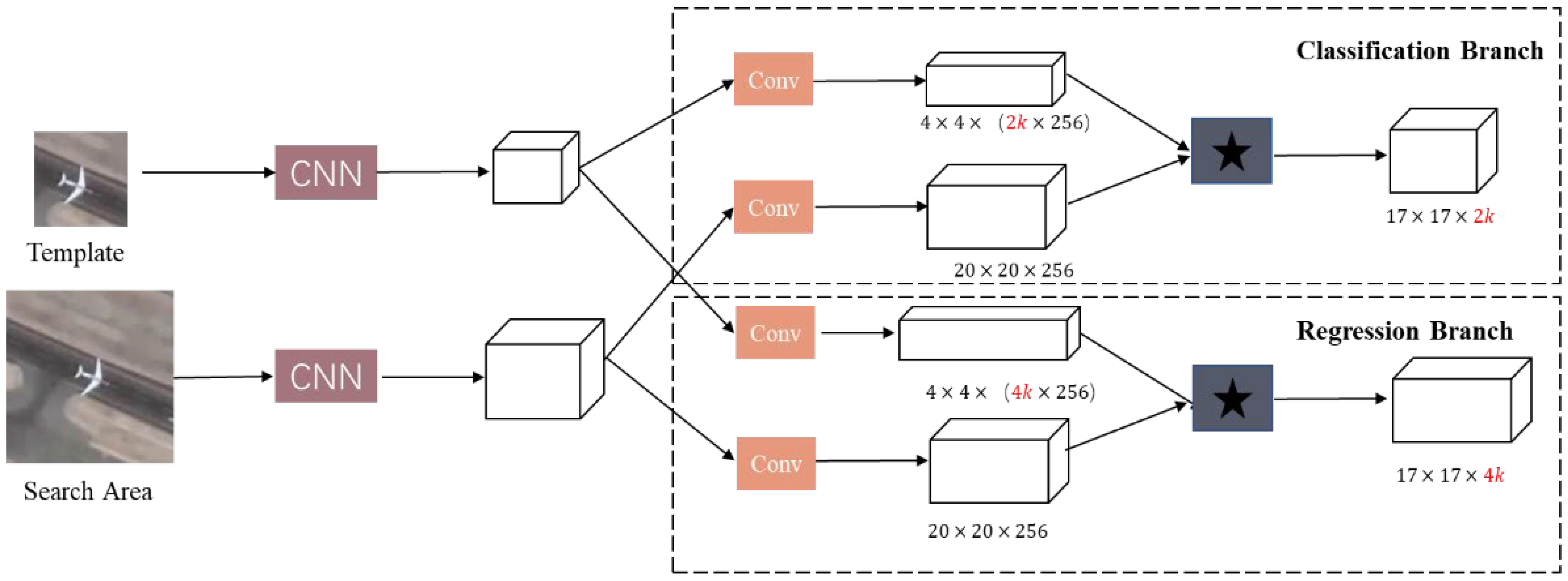
The trackers we choose are Siamese-RPN-based trackers, including SiamRPN, DaSiamRPN, and SiamRPN++, of which the backbones are AlexNet, ResNet, and MobileNet [57]. The gradient-based adversarial examples method we design is based on the fact that the models mentioned above use the RPN’s classification and regression branches to accurately locate the tracked object and tightly box it with anchor boxes. The RPN simultaneously sends fused features to the classification network and regression network for optimization of classification loss and regression loss during training. The overall framework of SiamRPN-like models can be seen in Figure 1.
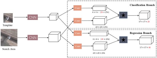
Figure 1.
The structure of SiamRPN-based trackers.
2.3.4. Methods
In this part, we introduce our attack method for trackers of RSI. Let T denote the template and S the search area of one image frame. Define and as the classification and regression cost functions, respectively. Then, the original lost function of the VOT task is given by Formula (5):
where M is the proposal number, λ is a weight coefficient, and and are the predicted labels for classification and regression, respectively. On the other hand, inspired by [58], we design our adversarial examples loss. Let denote the adversarial search area; therefore, the bounding box regression cost function can be expressed as Formula (6):
where is the pseudo-regression label conditioned on adversarial examples. In particular, is composed of four entries that represent the location of the bounding box. Thus, the entries for the adversarial label can be given by Formula (7):
where δ and represent the distance offset and scale variation, respectively. Therefore, the adversarial cost function targets making and the same when applying the predicted and pseudo-labels. Hence, the adversarial cost function can be expressed as Formula (8):
Now, we introduce the update rule for the adversarial search area. For the k-th frame, in light of the timeliness across frames, we partition all frames into multiple groups, each containing τ frames in order. Then, we take the perturbation of the (k − 1)-th frame as the initial perturbation of the k-th frame. Specifically, the adversarial search area of the k-th frame is given by Formula (9).
where is the index of the first frame in the corresponding group. Accordingly, the adversarial example is updated by the PGD as Formula (3).
Figure 2 illustrates the generation of RSI adversarial examples. The adversarial attack takes place in the test phase such that the model parameters are kept fixed. In particular, we solely add adversarial examples in the search area. Then, the detailed procedure can be described as follows. First, the clear template and the clear search area are input into the VOT tracker for feature extraction, followed by computing the gradients toward a cost function. We discuss the cost functions in the next subsections. Thereafter, the generated adversarial example, the search area, and the template are input into the VOT tracker for tracking. The main idea of this approach is to damage the weight parameters in the training phase by searching the gradient ascent direction.

Figure 2.
Pipeline of the generation of RSI adversarial examples.
The overall algorithm process is summarized in Algorithm 1 below.
| Algorithm 1: Adversarial Generation with , and Time Awareness. | ||
| Input: | Video frame , Template , search area , number of iterations frame interval | |
| Output: Adversarial search area , adversarial example | ||
| 1: Initialize: | ||
| 2: Compute: | ||
| 3: if r==1 then | ||
| 4: | ||
| 5: | = | |
| 6: else | ||
| 7: | for n = 1, … do | |
| 8: | Update by (9) | |
| 9: | Update by (10) | |
| 10: | end | |
| 11: | ||
| 12: | ||
| 13: end | ||
3. Results
This section introduces the evaluation metrics, details of the experiment, the final results, and the ablation experiment.
3.1. Evaluation Criteria
We adopt the evaluation standards of the natural dataset OTB [34], which mainly uses two types of evaluation indicators: Average Pixel Error (APE) and Average Overlap Rate (AOR). APE measures the average distance between the predicted bounding box and the ground truth bounding box, while AOR measures the average ratio of the intersection area to the union area between the predicted bounding box and the ground truth bounding box.
3.1.1. Average Pixel Error (APE)
APE, also known as a precision plot, refers to the average pixel distance between the predicted bounding box and the ground truth bounding box. It is a metric used to measure the closeness of two rectangles, where a larger value indicates a larger error. The APE value can be presented as a precision plot, which shows the percentage of videos where the distance between the two boxes is less than a given threshold. Different thresholds can yield different percentages, and a curve can thus be obtained. However, the drawback of this method is that it cannot reflect the variations in the size and scale of the target object.
3.1.2. Average Overlap Rate (AOR)
AOR is the average intersection over union (IoU) between the predicted bounding box and the ground truth, calculated over all frames in a video sequence. It is used to measure the degree of overlap between two boxes, indicating the success of object tracking. This can be presented as a Success plot, which shows the percentage of frames that have an IoU greater than a given threshold. The threshold value can vary, resulting in different percentages, and a curve can be plotted to represent the success rate. The range of values for the IoU threshold is 0 to 1. AOR can be represented by Formula (11). The formula calculates the overlap ratio between the predicted anchor box and the ground truth box, where O is the overlap ratio, is the predicted box, is the ground truth box, ∩ denotes the intersection of the two boxes, and ∪ denotes the union of the two boxes. The resulting ratio ranges from 0 to 1, with 1 indicating a perfect match between the predicted and ground truth boxes.
3.2. Implementation Details
Adversarial examples occur during the testing phase, so the model parameters are fixed. We use the pre-trained model parameters provided in Pysot (https://github.com/STVIR/pysot, accessed on 6 April 2023) for our method. In our approach, to ensure that the adversarial examples are imperceptible, we set τ = 10, which resets the adversarial example every 10 frames as we accumulate them frame by frame. For single-object tracking, to ensure real-time performance, we perform only two iterations of gradient descent per frame, with small steps and multiple iterations per frame to compensate. Therefore, N = 2, S = 0.3 in PGD attacks, and the original loss function λ = 5.
3.3. Results
To validate the effectiveness of our designed adversarial examples, we conduct attacks on trackers based on the RPN using adversarial examples on the SatSOT dataset and the VISO dataset. We select the DaSiamRPN, SiamRPN, and three different backbone models of SiamRPN++, where SiamRPN++_A represents the SiamRPN++ model based on AlexNet, SiamRPN++_M represents the SiamRPN++ model based on MobileNet, and SiamRPN++_R represents the SiamRPN++ model based on ResNet50. Table 1 shows the tracking results of the original datasets on the five models and the tracking results after incorporating our designed adversarial examples.

Table 1.
The attack performance of adversarial examples on the VOT model.
According to the results in the table, we find that the attack effect of DaSiamRPN is best, with the largest decrease in accuracy and precision. The attack effects of SiamRPN and SiamRPN++ models with different backbones are significant, but the overall attack effect is similar. Other SiamRPN algorithms can only distinguish the target from the background without semantic information and perform poorly when there is interference. That is, the DaSiamRPN model has better discrimination and focuses more on distinguishing background information. However, remote sensing images face serious challenges in visual object tracking tasks due to their large coverage area, severe occlusion, and small target size. Models that focus more on semantic background information are more susceptible to adversarial examples. In order to verify that the method of our adversarial examples generation is still effective against traditional 2D datasets, we conduct our attack method on OTB100 and UAV123 datasets. Table 2 shows the attack performance of adversarial examples against VOT models on OTB100 and UAV123 datasets. We can see that the precision results and success rates of the three trackers are significantly reduced after being attacked.

Table 2.
The attack performances of adversarial examples against VOT models on OTB100 and UAV123 datasets.
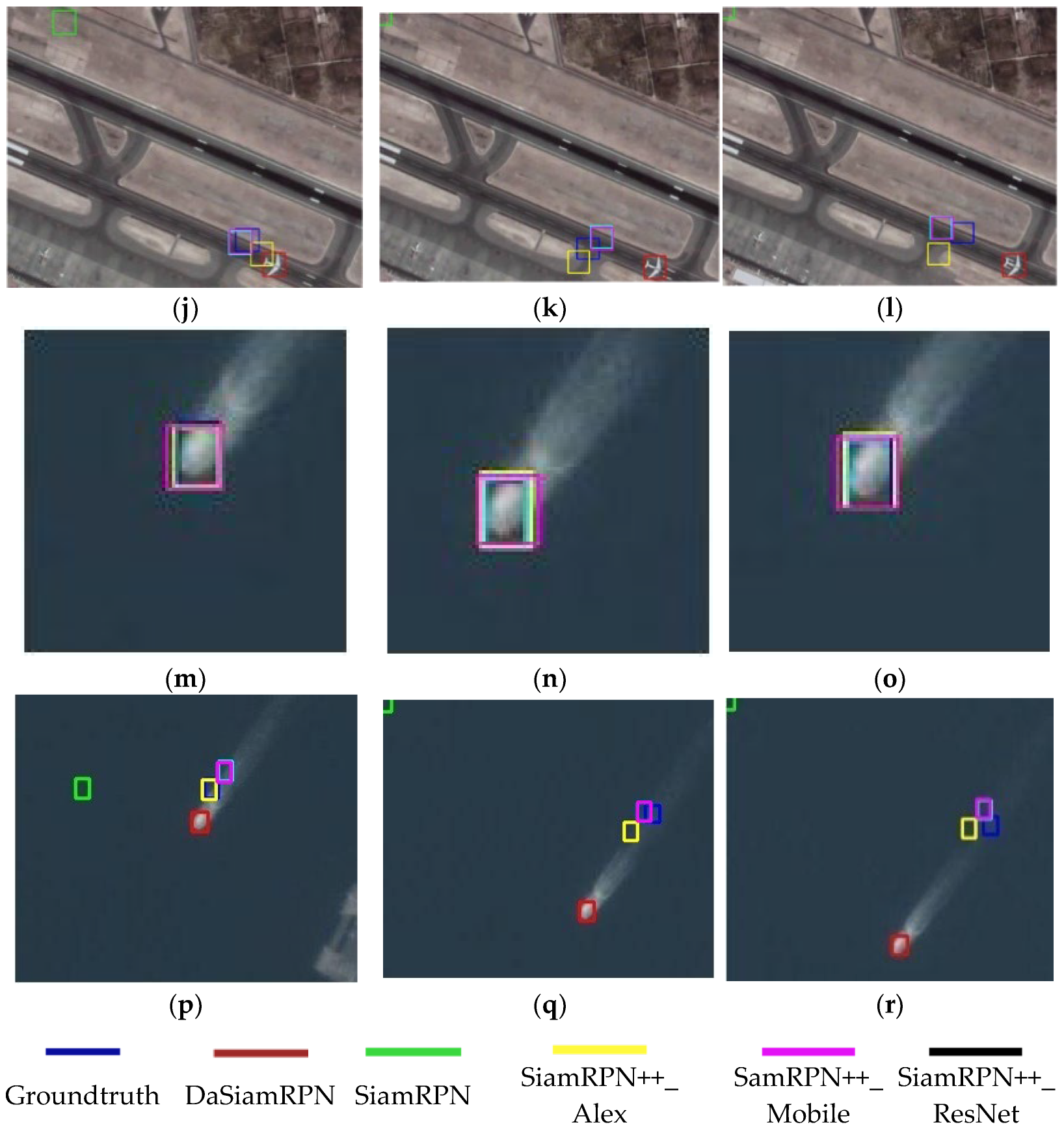
In order to illustrate the damage to the neural network model by adding video frames with adversarial examples, we show the tracking effect of 5 visual-object tracking models on 3 videos. The blue box represents the ground truth of the object. Boxes of other colors represent the tracking results of different models, while red represents the DASianRPN model, green represents the SiamRPN model, yellow box is the SiamRPN++ model based on AlexNet, the pink box is the SiamRPN++ model based on MobileNet, and the black box is the SiamRPN++ model based on ResNet. Each image shows the tracking results and ground truth for 5 VOT models. Specifically as shown in Figure 3.
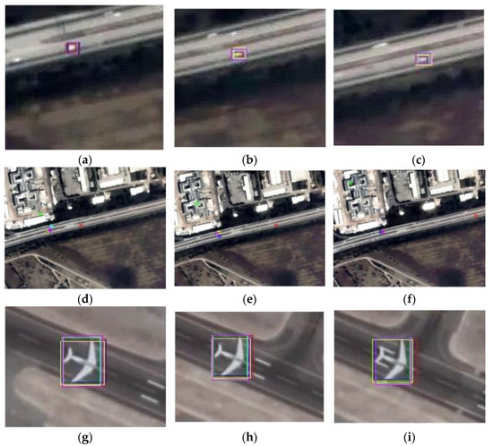
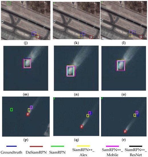
Figure 3.
Illustration the tracking results of 5 model in 3 videos with and without adversarial examples. (a) The original tracking result of the car at frame 100, (b) The original tracking result of the car at frame 200, (c) The original tracking result of the car at frame 300, (d) The attacked tracking result of the car at frame 100, (e) The attacked tracking result of the car at frame 200, (f) The attacked tracking result of the car at frame 300, (g) The original tracking result of the plane at frame 150, (h) The original tracking result of the plane at frame 300, (i) The original tracking result of the plane at frame 450, (j) The attacked tracking result of the plane at frame 150, (k) The attacked tracking result of the plane at frame 300, (l) The attacked tracking result of the plane at frame 450, (m) The original tracking result of the ship at frame 100, (n) The original tracking result of the ship at frame 200, (o) The original tracking result of the ship at frame 300, (p) The attacked tracking result of the ship at frame 100, (q) The attacked tracking result of the ship at frame 200, (r) The attacked tracking result of the ship at frame 300.
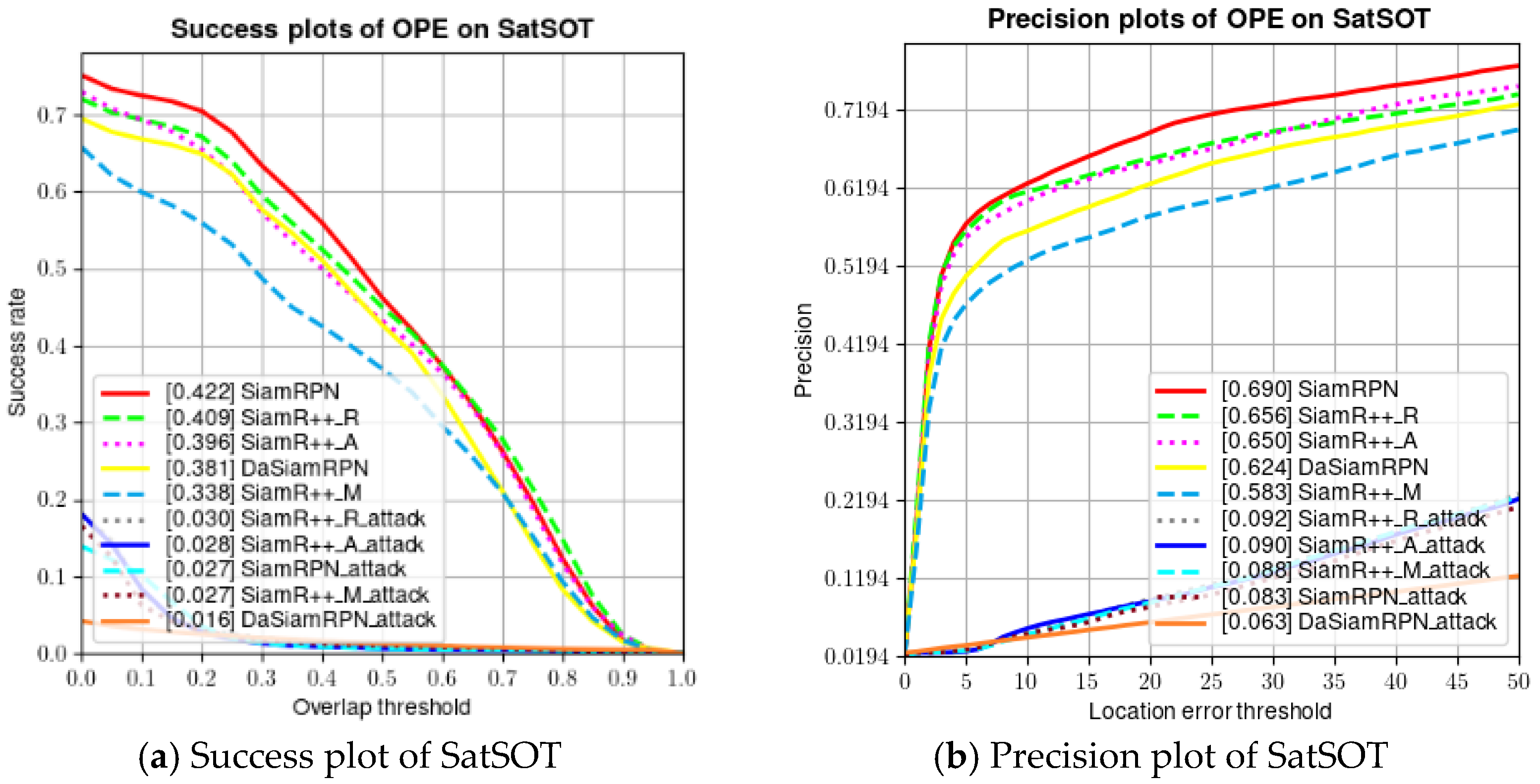
Figure 4 shows success plots and the precision plots on the SatSOT dataset. SiamRPN has the best performance on tracking the SatSOT dataset. From Figure 4, we can clearly see the damage of the adversarial example to the VOT model: both the success rate and accuracy of model tracking are greatly reduced.
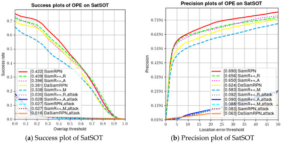
Figure 4.
Evaluation results of trackers without adversarial attacks on SatSOT dataset.
3.4. Ablation Experiment
To analyze the effect of classification loss and regression loss on the attack performance of the tracking model, we conduct ablation experiments on the loss functions as shown in Table 3. We select the SatSOT dataset, where represents the classification loss function and represents the regression loss function. We evaluate DaSiamRPN, SiamRPN, and SiamRPN++ based on AlexNet, MobileNet, and ResNet50. The results show that the attack performance is best when both loss functions are combined, resulting in the highest success rate and accuracy reduction of the tracking model.

Table 3.
Influence of classification loss and regression loss on attack effect.
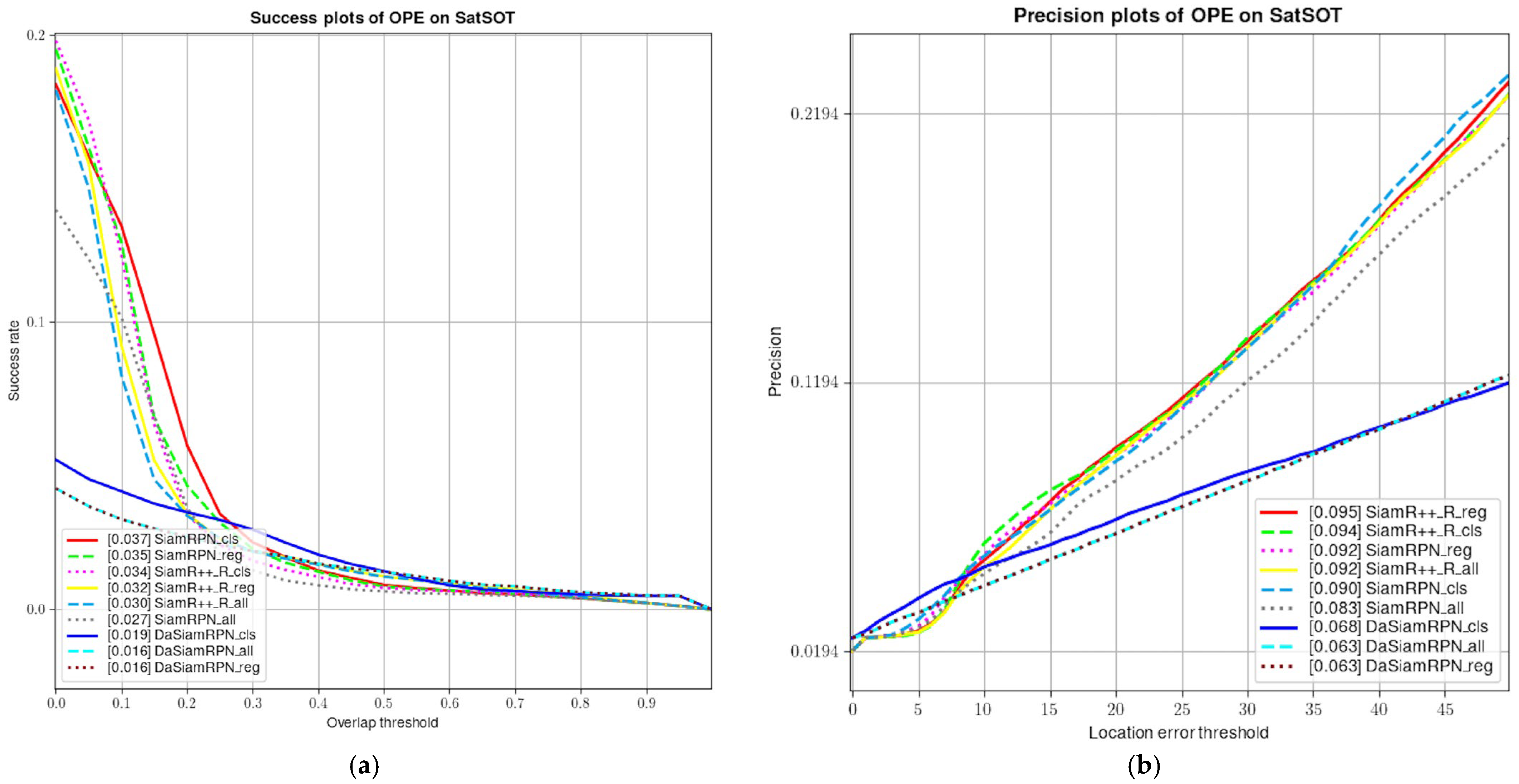
We conduct experiments on the SatSOT dataset using the SiamRPN++ model with a ResNet50 backbone. Specifically, we generate adversarial examples by adding only the classification loss, only the regression loss, or both loss functions simultaneously. The results are shown in Figure 5, which indicates that the adversarial examples generated by adding both loss functions have the best attack performance, followed by the adversarial examples generated by adding the regression loss function. This demonstrates the effectiveness of using multiple loss functions to generate adversarial examples in this scenario.
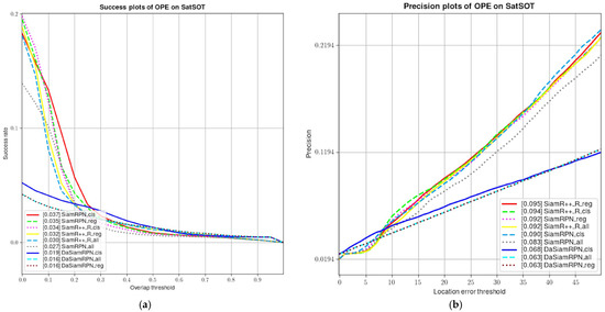
Figure 5.
The effect of different loss functions on the attack effect. (a) Success plot of attacked models on SatSOT, (b) Precision plot of attacked models on SatSOT.
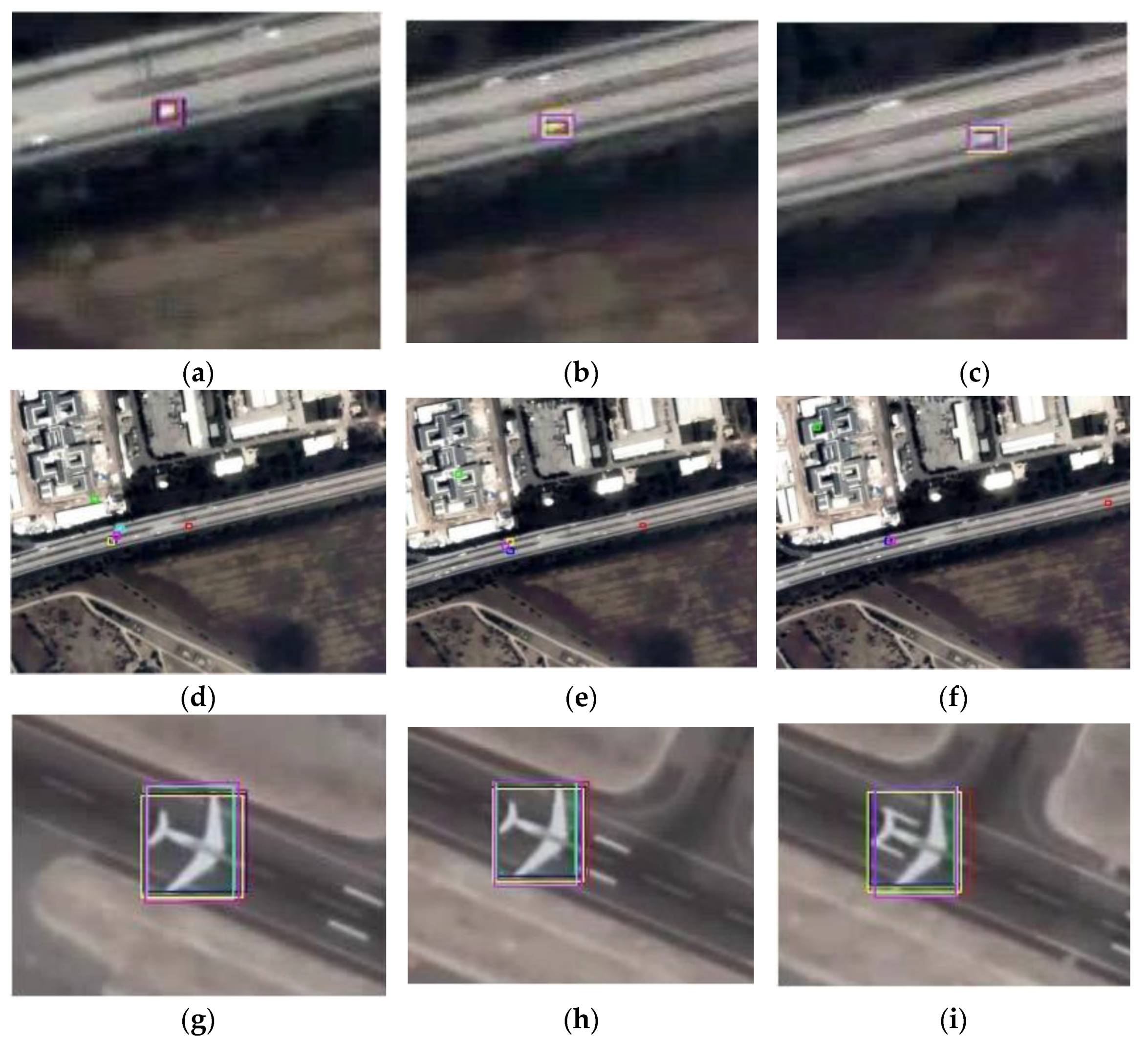
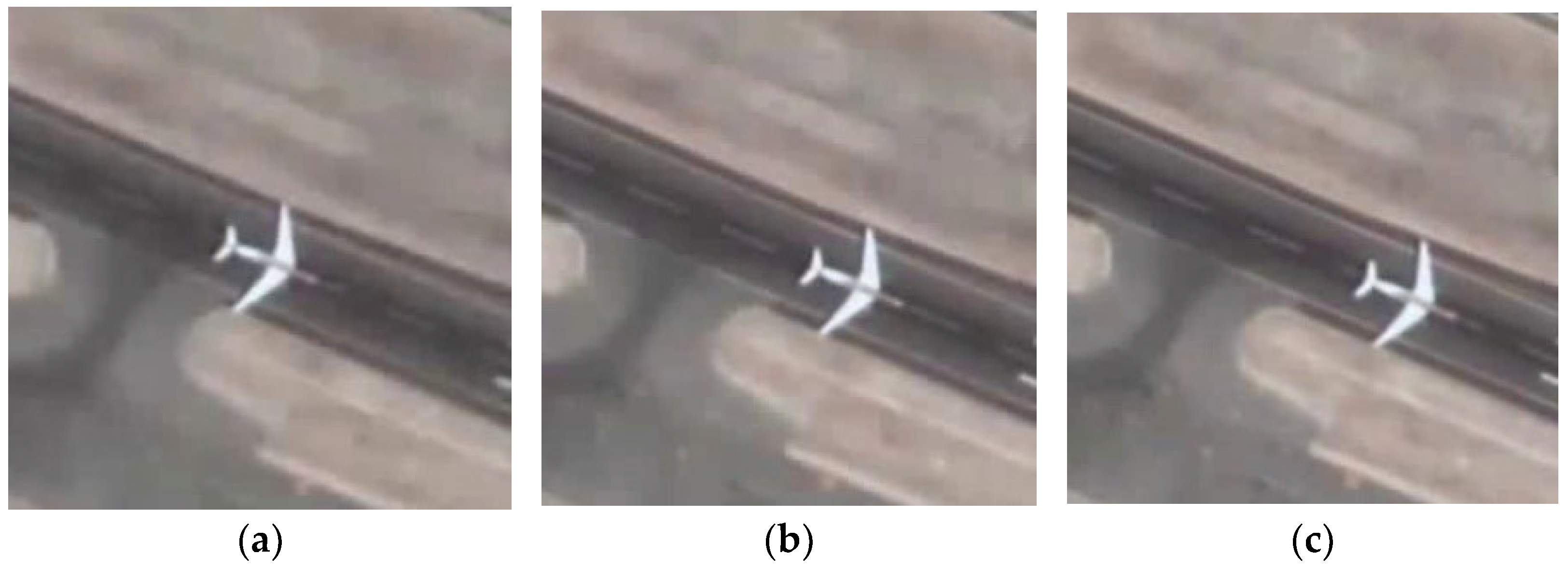
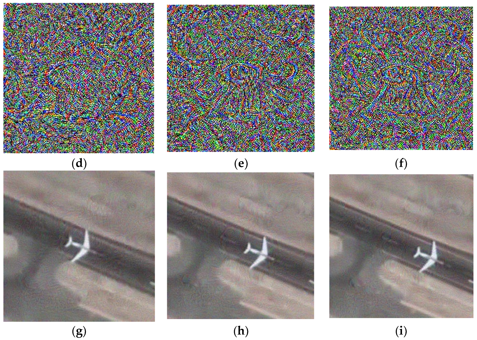
Adversarial examples are crafted with the intention to deceive machine learning models, and it is desirable to minimize the distortion to the original image while creating such examples. In this case, we present the original search regions, adversarial examples, and search regions with adversarial examples for the 5th, 100th, and 150th frames of the SatSOT dataset. Figure 6 showcases the obtained results by displaying the images, printing the adversarial examples, and comparing them with the original images. Through this evaluation, we can assess the effectiveness of adversarial examples and observe the impact of perturbations on the images. Notably, our adversarial examples not only lead to the failure of the tracking model but also possess the ability to deceive the human eye. In this evaluation process, we print the search regions that are fed into the neural network model, which are a small part of the entire input image. Due to the small size of the target in remote sensing images, adding adversarial examples to this part can not only reduce the computational resources required but also make the added perturbations more covert within the entire video frame. Therefore, our algorithm is proven to be an effective method for adversarial example generation, as it enhances the practicality and concealment of the attack while ensuring its effectiveness.
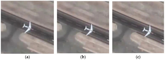

Figure 6.
A comparison between the original images and the images with added adversarial examples. The first row displays the search area of the neural network in the 5th, 100th, and 150th frames of the plane dataset. The second row shows the adversarial examples generated from the frames mentioned above. The third row displays the search area after adding the adversarial examples to the original frames. (a) Clear area of the 5th frame, (b) Clear area of the 100th frame, (c) Clear area of the 150th frame, (d) Adversarial example of the 5th frame, (e) Adversarial example of the 100th frame, (f) Adversarial example of the 150th frame, (g) Attacked area of the 5th frame, (h) Attacked area of the 100th frame, (i) Attacked area of the 150th frame.
4. Discussion
In this article, we explore for the first time the adversarial examples problem in the field of single-object tracking in remote sensing images. Remote sensing technology utilizes sensors on high-altitude platforms such as satellites and aircraft to observe and detect ground objects in a non-contact manner. Remote sensing can obtain remote sensing image data; monitor, measure, and analyze the Earth’s surface; and is widely used in fields such as agriculture, forestry, water conservancy, urban planning, environmental monitoring, meteorological forecasting, geological exploration, marine research, and military. Remote sensing technology can provide large-scale, multi-temporal, high-resolution, and high-precision geographic information, providing an important means for people to understand and explore the Earth. Remote sensing technology is widely used in various fields such as the military, resource exploration, environmental protection, disaster monitoring, and urban planning. In the military field, remote sensing technology can be used for reconnaissance and the monitoring of targets, supporting the formulation and implementation of combat plans. In the field of resource exploration, remote sensing technology can be used for mineral resource exploration and agricultural production monitoring. In the field of environmental protection, remote sensing technology can be used to monitor atmospheric pollution, water quality pollution, land degradation, etc. In the field of disaster monitoring, remote sensing technology can be used for rapid response and the loss assessment of disasters such as earthquakes, floods, and fires. In the field of urban planning, remote sensing technology can be used for urban planning, land use, and traffic management. Due to the ability of remote sensing technology to obtain large amounts of data and information, it has important application value in many fields. These important applications require a high robustness of deep learning models based on remote sensing.
In the field of visual object tracking, the RPN is often used as the downstream network model to approximate the position of the object and accurately frame the shape of the object. Based on this, we design a gradient-accumulation-based attack method for the RPN model commonly used in visual object tracking models. The RPN is composed of classification and regression branches. The classification branch mainly distinguishes the foreground and background of the region, and the regression branch divides the region into unequal proportions of anchor boxes to frame the target. Our intention for designing adversarial examples is to disrupt these two branches of the RPN. We confuse the ability of the classification module to distinguish between background and foreground, and give the regression branch a direction momentum so that it can be shifted while giving the anchor box a shrinking index and so that the shape of the anchor box gradually changes as the frame is pushed. Unlike the attack on static images in classification and detection, visual object tracking has a high requirement for the temporal consistency of the model. However, the adversarial examples generated by gradient-propagation-based methods are relatively time-consuming. To solve this problem, we consider the temporal consistency of the frame. We use small step iterations per frame to cumulatively add adversarial examples for each frame, instead of multiple iterations per frame. Through experiments and visualizations of perturbed images and original images, our adversarial examples can effectively disrupt the single-object tracking model. Our attack method is carried out in the digital domain, which only simulates the process of attacking the model. In the future, our work will focus on the physical domain, attacking in the real world.
5. Conclusions
In this paper, we proposed an adversarial examples method for visual object tracking in remote sensing images. By simultaneously designing classification and regression losses and utilizing the temporal information of video frames, our adversarial examples can accumulate across frames, leading to more effective attacks. We evaluated our method based on Region Proposal Networks (RPNs) on Siamese networks and demonstrated its effectiveness in attacking the model’s tracking performance. Our adversarial examples generation method not only renders the visual object tracking network ineffective but also deceives the human eye, making the attack more practical and harder to detect. Overall, our method presents a novel and effective approach for adversarial examples attacks in the field of remote sensing image analysis. We believe that this proposed method can contribute to the development of more robust and secure machine learning models for visual object tracking in remote sensing applications.
Author Contributions
Methodology and writing, Y.Z.; funding acquisition, J.L.; data curation, L.W. and C.Z. All authors have read and agreed to the published version of the manuscript.
Funding
This research received no external funding.
Data Availability Statement
Our datasets are all public datasets available at the links provided in the article.
Conflicts of Interest
The authors declare no conflict of interest.
References
- Depczyński, M.; Markiewicz, S.; Wrzosek, M. Challenges and Threats to Military Reconnaissance and Radio Combat from the Aspect of the Anti-Access System. J. Slav. Mil. Stud. 2022, 35, 73–93. [Google Scholar] [CrossRef]
- Bateman, A. Trust but verify: Satellite reconnaissance, secrecy and arms control during the Cold War. J. Strateg. Stud. 2023, 1–25. [Google Scholar] [CrossRef]
- Mirmina, S.; Schenewerk, C. National security and military uses of outer space. In International Space Law and Space Laws of the United States; Edward Elgar Publishing: Cheltenham, UK, 2022; pp. 272–293. [Google Scholar]
- Vohra, D.; Garg, P.K.; Ghosh, S. Real-time vehicle detection for traffic monitoring by applying a deep learning algorithm over images acquired from satellite and drone. Int. J. Intell. Unmanned Syst. 2022. [Google Scholar] [CrossRef]
- Pérez-Martínez, P.J.; Magalhães, T.; Maciel, I.; de Miranda, R.M.; Kumar, P. Effects of the COVID-19 pandemic on the air quality of the metropolitan region of São Paulo: Analysis based on satellite data, monitoring stations and records of annual average daily traffic volumes on the main access roads to the city. Atmosphere 2022, 13, 52. [Google Scholar] [CrossRef]
- van Lint, H.; Valkenberg, A.; van Binsbergen, A. Transitions towards Sustainable Mobility; Springer: Berlin/Heidelberg, Germany, 2011. [Google Scholar]
- Forrest, S.; Recio, M.; Seddon, P. Moving wildlife tracking forward under forested conditions with the SWIFT GPS algorithm. Anim. Biotelemetry 2022, 10, 19. [Google Scholar] [CrossRef]
- Webster, E.G.; Hamann, M.; Shimada, T.; Limpus, C.; Duce, S. Space-use patterns of green turtles in industrial coastal foraging habitat: Challenges and opportunities for informing management with a large satellite tracking dataset. Aquat. Conserv. Mar. Freshw. Ecosyst. 2022, 32, 1041–1056. [Google Scholar] [CrossRef]
- Mesquita, G.P.; Mulero-Pázmány, M.; Wich, S.A.; Rodríguez-Teijeiro, J.D. A practical approach with drones, smartphones, and tracking tags for potential real-time animal tracking. Curr. Zool. 2023, 69, 208–214. [Google Scholar] [CrossRef]
- Szegedy, C.; Zaremba, W.; Sutskever, I.; Bruna, J.; Erhan, D.; Goodfellow, I.; Fergus, R. Intriguing properties of neural networks. arXiv 2013, arXiv:1312.6199. [Google Scholar]
- Li, Y.; Zhong, H.; Ma, X.; Jiang, Y.; Xia, S.-T. Few-shot backdoor attacks on visual object tracking. arXiv 2022, arXiv:2201.13178. [Google Scholar]
- Saputro, D.R.S.; Widyaningsih, P. Limited memory Broyden-Fletcher-Goldfarb-Shanno (L-BFGS) method for the parameter estimation on geographically weighted ordinal logistic regression model (GWOLR). AIP Conf. Proc. 2017, 1868, 040009. [Google Scholar]
- Goodfellow, I.J.; Shlens, J.; Szegedy, C. Explaining and harnessing adversarial examples. arXiv 2014, arXiv:1412.6572. [Google Scholar]
- Madry, A.; Makelov, A.; Schmidt, L.; Tsipras, D.; Vladu, A. Towards deep learning models resistant to adversarial attacks. arXiv 2017, arXiv:1706.06083. [Google Scholar]
- Carlini, N.; Wagner, D. Towards evaluating the robustness of neural networks. In Proceedings of the 2017 IEEE Symposium on Security and Privacy (SP), San Jose, CA, USA, 22–26 May 2017; pp. 39–57. [Google Scholar]
- Czaja, W.; Fendley, N.; Pekala, M.; Ratto, C.; Wang, I.-J. Adversarial examples in remote sensing. In Proceedings of the 26th ACM SIGSPATIAL International Conference on Advances in Geographic Information System, Washington, DC, USA, 6–9 November 2018; pp. 408–411. [Google Scholar]
- Pang, Y.; Cheng, S.; Hu, J.; Liu, Y. Robust Satellite Image Classification with Bayesian Deep Learning. In Proceedings of the 2022 Integrated Communication, Navigation and Surveillance Conference (ICNS), Dulles, VA, USA, 5–7 April 2022; pp. 1–8. [Google Scholar]
- Papp, D.; Ma, Z.; Buttyan, L. Embedded systems security: Threats, vulnerabilities, and attack taxonomy. In Proceedings of the 2015 13th Annual Conference on Privacy, Security and Trust (PST), Izmir, Turkey, 21–23 July 2015; pp. 145–152. [Google Scholar]
- Pelletier, C.; Valero, S.; Inglada, J.; Champion, N.; Marais Sicre, C.; Dedieu, G. Effect of training class label noise on classification performances for land cover mapping with satellite image time series. Remote Sens. 2017, 9, 173. [Google Scholar] [CrossRef]
- Garrity, S.R.; Allen, C.D.; Brumby, S.P.; Gangodagamage, C.; McDowell, N.G.; Cai, D.M. Quantifying tree mortality in a mixed species woodland using multitemporal high spatial resolution satellite imagery. Remote Sens. Environ. 2013, 129, 54–65. [Google Scholar] [CrossRef]
- Tanıl, Ç.; Khanafseh, S.; Pervan, B. Detecting global navigation satellite system spoofing using inertial sensing of aircraft disturbance. J. Guid. Control Dyn. 2017, 40, 2006–2016. [Google Scholar] [CrossRef]
- Yu, D.-Y.; Ranganathan, A.; Locher, T.; Capkun, S.; Basin, D. Short paper: Detection of GPS spoofing attacks in power grids. In Proceedings of the 2014 ACM Conference on Security and Privacy in Wireless & Mobile Networks, Oxford, UK, 23–25 July 2014; pp. 99–104. [Google Scholar]
- Jovanovic, A.; Botteron, C.; Fariné, P.-A. Multi-test detection and protection algorithm against spoofing attacks on GNSS receivers. In Proceedings of the 2014 IEEE/ION Position, Location and Navigation Symposium-PLANS 2014, Monterey, CA, USA, 5–8 May 2014; pp. 1258–1271. [Google Scholar]
- Chen, L.; Zhu, G.; Li, Q.; Li, H. Adversarial example in remote sensing image recognition. arXiv 2019, arXiv:1910.13222. [Google Scholar]
- Chen, L.; Li, H.; Zhu, G.; Li, Q.; Zhu, J.; Huang, H.; Peng, J.; Zhao, L. Attack selectivity of adversarial examples in remote sensing image scene classification. IEEE Access 2020, 8, 137477–137489. [Google Scholar] [CrossRef]
- Kurakin, A.; Goodfellow, I.; Bengio, S. Adversarial machine learning at scale. arXiv 2016, arXiv:1611.01236. [Google Scholar]
- Xu, Y.; Du, B.; Zhang, L. Assessing the threat of adversarial examples on deep neural networks for remote sensing scene classification: Attacks and defenses. IEEE Trans. Geosci. Remote Sens. 2020, 59, 1604–1617. [Google Scholar] [CrossRef]
- Szegedy, C.; Liu, W.; Jia, Y.; Sermanet, P.; Reed, S.; Anguelov, D.; Erhan, D.; Vanhoucke, V.; Rabinovich, A. Going deeper with convolutions. In Proceedings of the IEEE Conference on Computer Vision and Pattern Recognition, Boston, MA, USA, 7–12 June 2015; pp. 1–9. [Google Scholar]
- He, K.; Zhang, X.; Ren, S.; Sun, J. Deep residual learning for image recognition. In Proceedings of the 2016 IEEE Conference on Computer Vision and Pattern Recognition (CVPR), Las Vegas, NV, USA, 27–30 June 2016; pp. 770–778. [Google Scholar]
- Krizhevsky, A.; Sutskever, I.; Hinton, G.E. Imagenet classification with deep convolutional neural networks. Commun. ACM 2017, 60, 84–90. [Google Scholar] [CrossRef]
- Jiang, Y.; Yin, G.; Yuan, Y.; Da, Q. Project gradient descent adversarial attack against multisource remote sensing image scene classification. Secur. Commun. Netw. 2021, 2021, 1–13. [Google Scholar] [CrossRef]
- Simonyan, K.; Zisserman, A. Very deep convolutional networks for large-scale image recognition. arXiv 2014, arXiv:1409.1556. [Google Scholar]
- Szegedy, C.; Vanhoucke, V.; Ioffe, S.; Shlens, J.; Wojna, Z. Rethinking the inception architecture for computer vision. In Proceedings of the 2016 IEEE Conference on Computer Vision and Pattern Recognition (CVPR), Las Vegas, NV, USA, 27–30 June 2016; pp. 2818–2826. [Google Scholar]
- Xu, Y.; Ghamisi, P. Universal adversarial examples in remote sensing: Methodology and benchmark. IEEE Trans. Geosci. Remote Sens. 2022, 60, 1–15. [Google Scholar] [CrossRef]
- Bai, T.; Wang, H.; Wen, B. Targeted Universal Adversarial Examples for Remote Sensing. Remote Sens. 2022, 14, 5833. [Google Scholar] [CrossRef]
- Lu, M.; Li, Q.; Chen, L.; Li, H. Scale-adaptive adversarial patch attack for remote sensing image aircraft detection. Remote Sens. 2021, 13, 4078. [Google Scholar] [CrossRef]
- Redmon, J.; Farhadi, A. Yolov3: An incremental improvement. arXiv 2018, arXiv:1804.02767. [Google Scholar]
- Girshick, R. Fast R-CNN. In Proceedings of the 2015 IEEE International Conference on Computer Vision (ICCV), Santiago, Chile, 7–13 December 2015; pp. 1440–1448. [Google Scholar]
- Zhang, Y.; Zhang, Y.; Qi, J.; Bin, K.; Wen, H.; Tong, X.; Zhong, P. Adversarial Patch Attack on Multi-Scale Object Detection for UAV Remote Sensing Images. Remote Sens. 2022, 14, 5298. [Google Scholar] [CrossRef]
- Deng, B.; Zhang, D.; Dong, F.; Zhang, J.; Shafiq, M.; Gu, Z. Rust-Style Patch: A Physical and Naturalistic Camouflage Attacks on Object Detector for Remote Sensing Images. Remote Sens. 2023, 15, 885. [Google Scholar] [CrossRef]
- Danelljan, M.; Bhat, G.; Khan, F.S.; Felsberg, M. Atom: Accurate tracking by overlap maximization. In Proceedings of the 2019 IEEE/CVF Conference on Computer Vision and Pattern Recognition (CVPR), Long Beach, CA, USA, 15–20 June 2019; pp. 4660–4669. [Google Scholar]
- Bhat, G.; Danelljan, M.; Gool, L.V.; Timofte, R. Learning discriminative model prediction for tracking. In Proceedings of the IEEE/CVF International Conference on Computer Vision, Seoul, Republic of Korea, 2 November 2019; pp. 6182–6191. [Google Scholar]
- Zhang, D.; Zheng, Z.; Li, M.; He, X.; Wang, T.; Chen, L.; Jia, R.; Lin, F. Reinforced similarity learning: Siamese relation networks for robust object tracking. In Proceedings of the 28th ACM International Conference on Multimedia, Seattle, WA, USA, 12–16 October 2020; pp. 294–303. [Google Scholar]
- Bertinetto, L.; Valmadre, J.; Henriques, J.F.; Vedaldi, A.; Torr, P.H. Fully-convolutional siamese networks for object tracking. In Proceedings of the Computer Vision–ECCV 2016 Workshops, Amsterdam, The Netherlands, 8–10, 15–16 October 2016; Part II 14. pp. 850–865. [Google Scholar]
- Li, B.; Yan, J.; Wu, W.; Zhu, Z.; Hu, X. High performance visual tracking with siamese region proposal network. In Proceedings of the 2018 IEEE/CVF Conference on Computer Vision and Pattern Recognition, Salt Lake City, UT, USA, 18–23 June 2018; pp. 8971–8980. [Google Scholar]
- Zhu, Z.; Wang, Q.; Li, B.; Wu, W.; Yan, J.; Hu, W. Distractor-aware siamese networks for visual object tracking. In Proceedings of the European Conference on Computer Vision (ECCV), Munich, Germany, 8–14 September 2018; pp. 101–117. [Google Scholar]
- Li, B.; Wu, W.; Wang, Q.; Zhang, F.; Xing, J.; Yan, J. Siamrpn++: Evolution of siamese visual tracking with very deep networks. In Proceedings of the 2019 IEEE/CVF Conference on Computer Vision and Pattern Recognition (CVPR), Long Beach, CA, USA, 15–20 June 2019; pp. 4282–4291. [Google Scholar]
- Liang, S.; Wei, X.; Yao, S.; Cao, X. Efficient adversarial attacks for visual object tracking. In Proceedings of the Computer Vision–ECCV 2020: 16th European Conference, Glasgow, UK, 23–28 August 2020; Part XXVI 16. pp. 34–50. [Google Scholar]
- Chen, X.; Yan, X.; Zheng, F.; Jiang, Y.; Xia, S.-T.; Zhao, Y.; Ji, R. One-shot adversarial attacks on visual tracking with dual attention. In Proceedings of the IEEE/CVF Conference on Computer Vision and Pattern Recognition, Seattle, WA, USA, 14–19 June 2020; pp. 10176–10185. [Google Scholar]
- Liu, S.; Chen, Z.; Li, W.; Zhu, J.; Wang, J.; Zhang, W.; Gan, Z. Efficient universal shuffle attack for visual object tracking. In Proceedings of the ICASSP 2022-2022 IEEE International Conference on Acoustics, Speech and Signal Processing (ICASSP), Singapore, 23–27 May 2022; pp. 2739–2743. [Google Scholar]
- Chen, X.; Fu, C.; Zheng, F.; Zhao, Y.; Li, H.; Luo, P.; Qi, G.-J. A Unified Multi-Scenario Attacking Network for Visual Object Tracking. In Proceedings of the AAAI Conference on Artificial Intelligence, Online, 2–9 February 2019; pp. 1097–1104. [Google Scholar]
- Yan, X.; Chen, X.; Jiang, Y.; Xia, S.-T.; Zhao, Y.; Zheng, F. Hijacking tracker: A powerful adversarial attack on visual tracking. In Proceedings of the ICASSP 2020-2020 IEEE International Conference on Acoustics, Speech and Signal Processing (ICASSP), Barcelona, Spain, 4–8 May 2020; pp. 2897–2901. [Google Scholar]
- Yin, Q.; Hu, Q.; Liu, H.; Zhang, F.; Wang, Y.; Lin, Z.; An, W.; Guo, Y. Detecting and tracking small and dense moving objects in satellite videos: A benchmark. IEEE Trans. Geosci. Remote Sens. 2021, 60, 1–18. [Google Scholar] [CrossRef]
- Zhao, M.; Li, S.; Xuan, S.; Kou, L.; Gong, S.; Zhou, Z. SatSOT: A benchmark dataset for satellite video single object tracking. IEEE Trans. Geosci. Remote Sens. 2022, 60, 1–11. [Google Scholar] [CrossRef]
- Mueller, M.; Smith, N.; Ghanem, B. A benchmark and simulator for uav tracking. In Proceedings of the Computer Vision–ECCV 2016: 14th European Conference, Amsterdam, The Netherlands, 11–14 October 2016; Proceedings Part I 14. pp. 445–461. [Google Scholar]
- Wu, Y.; Lim, J.; Yang, M.H. Object tracking benchmark. IEEE Trans. Pattern Anal. Mach. Intell. 2015, 37, 1834–1848. [Google Scholar] [CrossRef] [PubMed]
- Howard, A.G.; Zhu, M.; Chen, B.; Kalenichenko, D.; Wang, W.; Weyand, T.; Andreetto, M.; Adam, H. Mobilenets: Efficient convolutional neural networks for mobile vision applications. arXiv 2017, arXiv:170404861. [Google Scholar]
- Jia, S.; Ma, C.; Song, Y.; Yang, X. Robust tracking against adversarial attacks. In Proceedings of the European Conference on Computer Vision, Glasgow, UK, 23–28 August 2020; pp. 69–84. [Google Scholar]
Disclaimer/Publisher’s Note: The statements, opinions and data contained in all publications are solely those of the individual author(s) and contributor(s) and not of MDPI and/or the editor(s). MDPI and/or the editor(s) disclaim responsibility for any injury to people or property resulting from any ideas, methods, instructions or products referred to in the content. |
© 2023 by the authors. Licensee MDPI, Basel, Switzerland. This article is an open access article distributed under the terms and conditions of the Creative Commons Attribution (CC BY) license (https://creativecommons.org/licenses/by/4.0/).

