Article

Adapting an Existing Empirical Algorithm for Microwave Land Surface Temperature Retrieval in China for AMSR2 Data

1
Shaanxi Key Laboratory of Earth Surface System and Environmental Carrying Capacity, College of Urban and Environmental Sciences, Northwest University, Xi’an 710127, China
2
Institute of Earth Surface System and Hazards, College of Urban and Environmental Sciences, Northwest University, Xi’an 710127, China
3
State Key Laboratory of Tibetan Plateau Earth System, Environment and Resources, Institute of Tibetan Plateau Research, Chinese Academy of Sciences, Beijing 100101, China
*
Author to whom correspondence should be addressed.
Remote Sens. 2023, 15(13), 3228; https://doi.org/10.3390/rs15133228
Submission received: 15 May 2023 / Revised: 19 June 2023 / Accepted: 20 June 2023 / Published: 22 June 2023

Abstract

:
To extend the time span of the microwave (MW) land surface temperature (LST) dataset in China, this study proposed an optimized empirical algorithm for Advanced Microwave Scanning Radiometer 2 (AMSR2) LST retrieval based on the algorithm for its predecessor, the AMSR-Earth Observing System (AMSR-E). A modified comprehensive classification system of environmental variables (CCSEV) that considered the impact of landform, landcover, atmospheric conditions, and solar radiation on the variation of LST was first constructed, and the LST for each class in the CCSEV was then retrieved through stepwise regression using the brightness temperature in different AMSR2 channels. The results indicate that the annual RMSE of the AMSR2 LST, compared to the reference Moderate Resolution Imaging Spectroradiometer (MODIS) LST from 2012 to 2020, varies between 3.26 K and 3.61 K in the daytime and 2.76 K and 2.96 K in the nighttime, respectively. The RMSE of the AMSR2 LST compared to the field measurements at the sites of the Beidahe river basin and Naqu regions varies between 4.16 K and 5.26 K in the daytime and 2.4 K and 5.17 K in the nighttime. The accuracy is relatively low in the warmer months and daytime due to the stronger solar radiation, and is also relatively low in western China due to the dominate highly fluctuating topography and barren and arid landcover. Generally, the accuracy of the AMSR2 LST is comparable with that of the AMSR-E LST retrieved by the predecessor algorithm, which facilitates coherent long-term applications using AMSR series LST datasets.

1. Introduction

Land surface temperature (LST) is an important parameter of the Earth’s surface and has a significant impact on the ecological system of the Earth. It is a reflection of the distribution of heat energy on the Earth’s surface and impacts various ecological elements such as the atmosphere, soil, water, vegetation, animals, and microbes [1,2,3,4,5,6,7], etc. For example, the LST affects the heat exchange near the surface, which can create different weather, change the form of water and soil, promote or inhibit the growth of plants and microbes, and impact the activity of animals. Remote sensing technology is a practical way to obtain surface parameters, including the LST, on a large spatial scale, which significantly benefits the above-mentioned research areas.
LST retrieval algorithms for thermal infrared (TIR) are currently well-developed and achieve high accuracy. They are already applied to retrieve LST products from various TIR [8,9,10,11,12] sensors. However, these products are restricted to clear-sky conditions and characterized by serious spatiotemporal discontinuities [13] because the TIR signal cannot penetrate clouds. Passive microwave (MW), by contrast, has the ability to penetrate clouds and exhibits unique advantages in all-weather applications; however, the generated LST data have the defect of lower spatial resolution and accuracy. The fusion of MW and TIR LSTs is an effective method to develop all-weather LSTs with a higher resolution [13,14,15,16,17,18], and can synthesize the advantages of both TIR and MW LSTs. Accordingly, improving the accuracy of MW LST retrieval is a critical factor that determines the quality of fused spatial continuous LST data.
Many studies have focused on the retrieval of the LST from different MW sensors [19,20,21,22,23,24]. The algorithms for MW LST retrieval are generally grouped into physical models, empirical statistical models, and machine learning models, in which empirical statistical models are most commonly applied due to their simplicity. This type of model retrieves the LST based on the regression relationship between the MW brightness temperature (BT) and reference LST (e.g., in situ measurements and TIR products); therefore, they do not need to deal with the complex radiation transfer processes and parameters in the radiation transfer equation (RTE). Nevertheless, they are usually region-specific in order to ensure accuracy. The exploration of proper channel combinations and spatiotemporal partitions are the two major concerns for the development of empirical statistical models. For channel combinations, McFarland, Miller, and Neale [20] pointed out that the most applicable channels for MW LST retrieval are vertical polarized 37 and 89 GHz. Subsequently, several studies concluded that two sets of vertical polarized channel differences are able to reduce the impact of soil moisture and water vapor—including 36.5 GHz minus 23.8 GHz and 36.5 GHz minus 18.7 GHz [25,26]—and that the quadratic items can further improve the accuracy [27]. For spatiotemporal partitions, combining different multiple regression models designed for specific environmental conditions has been preferred by researchers, given that the LST is comprehensively affected by various environmental factors. McFarland, Miller, and Neale [20] retrieved the MW LST in the Great Plains of the United States by combining the regression models designed for different landcover (LC) types. Then, Hollinger [28] and Owe and Van De Griend [26] introduced the seasonal and diurnal timescale into the algorithm. Zhou, Dai, Zhang, Zhao, and Li [23] established a classification system to retrieve the LST involving diurnal and seasonal timescales and various LC types, and Zhang and Cheng [29] further optimized the seasonal timescale to months and introduced the influence of topography on LST retrieval.
Advanced Microwave Scanning Radiometers on satellite Aqua (AMSR-E) and satellite Global Change Observation Mission 1st-Water (AMSR2) are MW sensors that share an identical transit time with the TIR sensor Moderate Resolution Imaging Spectroradiometer (MODIS) on Aqua. The BT data from these two MW sensors, joining with MODIS LST, are therefore regularly used in the study of LST fusion. To improve the quality of the fused all-weather LST data [18], Zhang and Cheng [29] proposed a comprehensive classification system of environmental variables (CCSEV) consisting of LC, topography, and near-surface air conditions to retrieve the AMSR-E LST using a stepwise regression model. This algorithm inherited and improved the mechanism of channel combinations and spatiotemporal partitions of the current empirical statistical models and has a relatively high accuracy compared with other contemporary algorithms. However, AMSR-E only provides data for 10 years—from August 2002 to September 2011—which does not meet the requirement of regional and global climate research on all-weather LST data for the long-term in order to review the variation in the climate-related parameters in the past and predict their trend in the future. AMSR2, which provides data beginning in July 2012, succeed AMSR-E, and has a higher spatial resolution and an additional channel at 7.3 GHz. Therefore, this study proposed an optimized algorithm for AMSR2 LST retrieval based on that developed by Zhang and Cheng [29] to promote the development of a long-term all-weather LST dataset, in which some defects that impact the retrieving accuracy have been fixed. The improvements mainly include: (1) The MODIS LC [30] and snow cover products [31] used to construct the CCSEV were replaced by more accurate GlobeLand30 LC [32] and new MODIS snow cover extent (SCE) [31] products in China to partition the boundaries of zones more accurately; (2) The number of zones of landform and vegetated LC and bareland was reduced from 71 to 62 to avoid the incapability of establishing the regression models in some classes due to their too-small volume; (3) The quality control of the MW BT data was more strict to exclude the impact of outlier values; (4) The replacement strategy of models in the classes with insufficient training samples was optimized to restrict the unreasonable growth of root mean square error (RMSE). In addition, some other processes in the LST retrieval were adjusted to fit the AMSR2 data as the number of BT channels was increased from 12 to 14, and the spatial resolution of the BT data was improved from 25 km to 10 km.

2. Study Area and Data

2.1. Study Area

The optimized algorithm for retrieving the AMSR2 LST was applied in the landmass of China (Figure 1), a landscape characterized by diverse and intricate environments. The terrain of China is mainly separated by three steps, with the altitude decreasing from the west to the east. The first step is the Qinghai-Tibet Plateau (QTP), located in the southwestern part of China, which includes high mountains, hills, and basins. The second step is located in the northwestern and central parts and includes mountains, hills, basins, and plateaus. The third step is located in the eastern part and includes plains and hills. The LC types are also varied, covering the whole landmass, comprised of forest, shrubland, cultivated land, grassland, tundra, waterbody, wetland, bareland, artificial surfaces, and glaciers, etc. The climates here include equatorial monsoon, warm temperature, desert, steppe, tundra, and snow types, etc. [33], ranging from tropic zones to cold zones, coastal to inland, and low altitude to high altitude. This specific environment of China makes LST retrieval more challenging.
The verification sites in the Beidahe River Basin (BRB) and Naqu region are used to evaluate the accuracy of the retrieved AMSR2 LST. These sites are located in QTP and its neighboring areas, a region that has a significant impact on the climatic characteristics in Central Asia. The BRB region is in the range of 39°00′–39°50′N and 97°15′–98°15′E. It pertains to the climate type of the transition from cold desert to tundra, and the topography is relatively fluctuating (average slope 14.22°). The Naqu region is in the range of 30°55′–31°10′N and 91°35′–91°50′E. It pertains to the tundra climate, and the topography is relatively gentle (average slope 6.94°). The LCs in these two regions are mainly bareland and grassland. Glaciers are also scattered at the summit or valley of some mountains in both regions, which are important sources of water for the river in the lower reaches.

2.2. Data

2.2.1. Satellite Data

The AMSR2 sensor includes horizontal and vertical polarized channels distributed in seven frequencies (6.9, 7.3, 10.7, 18.7, 23.8, 36.5 and 89 GHz). The transit time of AMSR2 is local 1:30 a.m. and 1:30 p.m., respectively. The level 3 AMSR2 BT dataset with 10 km resolution was adopted, which was obtained from the Japan Aerospace Exploration Agency (https://suzaku.eorc.jaxa.jp/GCOM_W/index.html (accessed on 1 June 2023)).
The MODIS level 3 LST product (MYD11A1) from the satellite Aqua was adopted as the reference because it shares an identical transit time with AMSR2. MYD11A1 consists of daily daytime and nighttime LST and corresponding quality control data. The MODIS LST dataset has an accuracy greater than 1 K over homogeneous surface [34]. The MYD11A1 dataset was obtained from the Land Processes Distributed Active Archive Center (https://ladsweb.modaps.eosdis.nasa.gov/ (accessed on 1 June 2023)).
The LC product GlobeLand30 [32] from the National Geomatics Center of China (http://www.ngcc.cn/ (accessed on 1 June 2023)) was adopted to construct the CCSEV. This product integrates the multispectral images from Landsat TM5, ETM+, OLI, Huanjing-1, and Gaofen-1. The current version consists of three annual datasets, including 2000, 2010, and 2020. For the region of China, the comparison with six other open LC products, including the widely applied MODIS product, found that GlobeLand30 has the highest overall accuracy of 82.4%. Although only 3 years of datasets with a 10-year interval were available, the annual GlobeLand30 dataset closest to the current year of AMSR2 was used to establish the annual CCSEV, considering that the interannual variation of LC among the adjacent years was negligible at the AMSR2 pixel scale.
The daily variation of snow cover also impacts the LST distribution, although it is not reflected in the annual LC datasets. A new MODIS SCE product over China [35], provided by the National Tibetan Plateau Third Pole Environment Data Center (https://data.tpdc.ac.cn/ (accessed on 1 June 2023)), is adopted in the construction of the CCSEV. This product has an overall accuracy of 93.15%, which is higher than the original MODIS snow cover product, MYD10A1F, by approximately 8.8%.
The elevation product from the Shuttle Radar Topography Mission (SRTM) was obtained in February 2000 and covers the land surface of the Earth between 60°N to 56°S. This product possesses relatively high accuracy and resolution [36], and has thus been used in many fields since its release [37,38]. There are two types of resolution for SRTM elevation data: 1″ and 3″. The 3″ resolution data is applied due to its wider applications and is downloaded from the Consultative Group on International Agricultural Research Consortium for Spatial Information (https://srtm.csi.cgiar.org/ (accessed on 1 June 2023)).

2.2.2. The Desert and Glacier Distribution Data

The dataset of desert in China [39] was produced on the basis of the aerial survey and field investigation conducted in the 1970s. This dataset maps the primary desert regions in the northern part of China, which was obtained from the Cold and Arid Regions Science Data Center (http://www.ncdc.ac.cn (accessed on 1 June 2023)). It is found that the GlobeLand30 mixed up a large proportion of glacier (i.e., permanent snow and ice) pixels with other LCs including cloud, bareland, grassland, and daily changing snow cover. Therefore, the Randolph Glacier Inventory version 6.0 (RGI 6.0) [40] was adopted to substitute for the glacier extent in the GlobeLand30 datasets, which was download from the Global Land Ice Measurements from Space website (http://www.glims.org/ (accessed on 1 June 2023)). It is assumed that in the AMSR2 pixel scale, the variation of glacier outlines from 2012 to 2020 can be ignored. The glacier pixels in GlobeLand30 that were not recognized as glaciers in RGI 6.0 were designated as the nearby LC types.

2.2.3. Soil Temperature Data

Compared with the surface temperature, the soil temperature is more commonly used to verify the accuracy of satellite-retrieved LST [15,18,41] because it is easier to measure and forms an observation network with a large coverage area. The field soil temperature measurements of the Naqu region came from the Central Tibet Plateau Soil Moisture and Temperature Monitoring Network (CTP-SMTMN, http://ismn.geo.tuwien.ac.at/ (accessed on 1 June 2023)), which collects the soil moisture and temperature observations at multiple depths every 30 min. The sites in this network are distributed along the roads in the Naqu region, with a relatively flat local terrain and altitudes ranging between 4468 m and 4837 m. The LC types of these sites are grassland and bareland. The observations at 0–5 cm deep were employed because they are the closest to the land surface. The field observations in the BRB region were collected by the authors using the Onset MX 2201 sensor, which recorded the soil temperature at 0–5 cm deep every 5 min at three sites, i.e., the Yumendong (YMD) site, the Diaodabangou (DDB) site, and the Qiyi Glacier (QYG) site (Figure 1). These three sites are placed at relatively flat local terrains with altitudes of 2350 m, 3450 m, and 4668 m, respectively. The LC types of these sites are bareland, grassland, and ice and snow. For AMSR2 LST validation, the soil temperature observations of the Naqu and BRB sites at the transit time of AMSR2 pixels were retained.

3. Method

3.1. The Theory of AMSR2 LST Retrieval

The MW RTE [27] expresses the components of MW radiation captured by the sensor and is the basis of MW LST retrieval.
T b = e τ T s + 1 e 1 τ τ T a   e w + 1 τ T a   s w
where Tb is the BT captured by the MW sensor in Kelvin (K), Ts is the LST in K, Ta ew and Ta sw are the mean atmospheric temperatures in the earthward and skyward directions in K; τ is the atmospheric transmittance and e is the land surface emissivity. This equation indicates the five parameters required to calculate the LST. Among them, Tb is a known parameter, e is relevant to the physical properties of specific LC and varies with the terrain fluctuation and the observation angle of the sensor. τ, Ta ew and Ta sw are relevant to the atmospheric components and solar radiation and change in space and time. With the exception of Tb, the accurate values of the remaining parameters are not easy to acquire on a large spatial scale.
Equation (1) shows that the LST and BT have a linear relationship, given e, τ, Ta ew and Ta sw, and this finding supports the application of the empirical statistical method to derive the LST from the MW BT in different environmental states. Therefore, the retrieval model of the MW LST can be written as the regression equation under the restriction of these environmental parameters, i.e.,
T s = f T b , T o p o ,   L , t , s
where Topo, L, t, and s are the restriction conditions of topography, LC, time, and space, respectively. To ensure the accuracy, a CCSEV based on these conditions is first constructed, where the inner homogeneity of each class should be as high as possible, and the f for each class is then regressed.
Based on the regression equation for the AMSR-E LST [29] and considering the number of AMSR2 channels, the initial equation for AMSR2 LST retrieval can be expressed as:
T s = A 0 + i = 1 7 A i h T b i h + A i v T b i v + B T b 36.5 v T b 18.7 v 2 + C T b 36.5 v T b 23.8 v 2 ,
where i represents the seven frequencies of AMSR2; h and v are the horizontal and vertical polarization; A0, Ai, B, C represent the coefficients of the prediction terms. All 14 channels of AMSR2 and the two additional quadratic terms for soil moisture and water vapor correction are involved in view of the complicated landscapes in China. Then, the stepwise regression is adopted to eliminate the unnecessary terms for the certain classes in which the participation of all the items may not achieve the best retrieval.

3.2. Estabishing the CCSEV

Although the LC datasets are replaced by more accurate ones, the number of zones for landform and LC decreases, and the minimum partition unit (i.e., the pixel size of AMSR2 BT data) shrinks, the procedure for establishing the annual CCSEV for AMSR2 LST retrieval is generally similar to that for AMSR-E [29], consisting of four major steps (Figure 2).
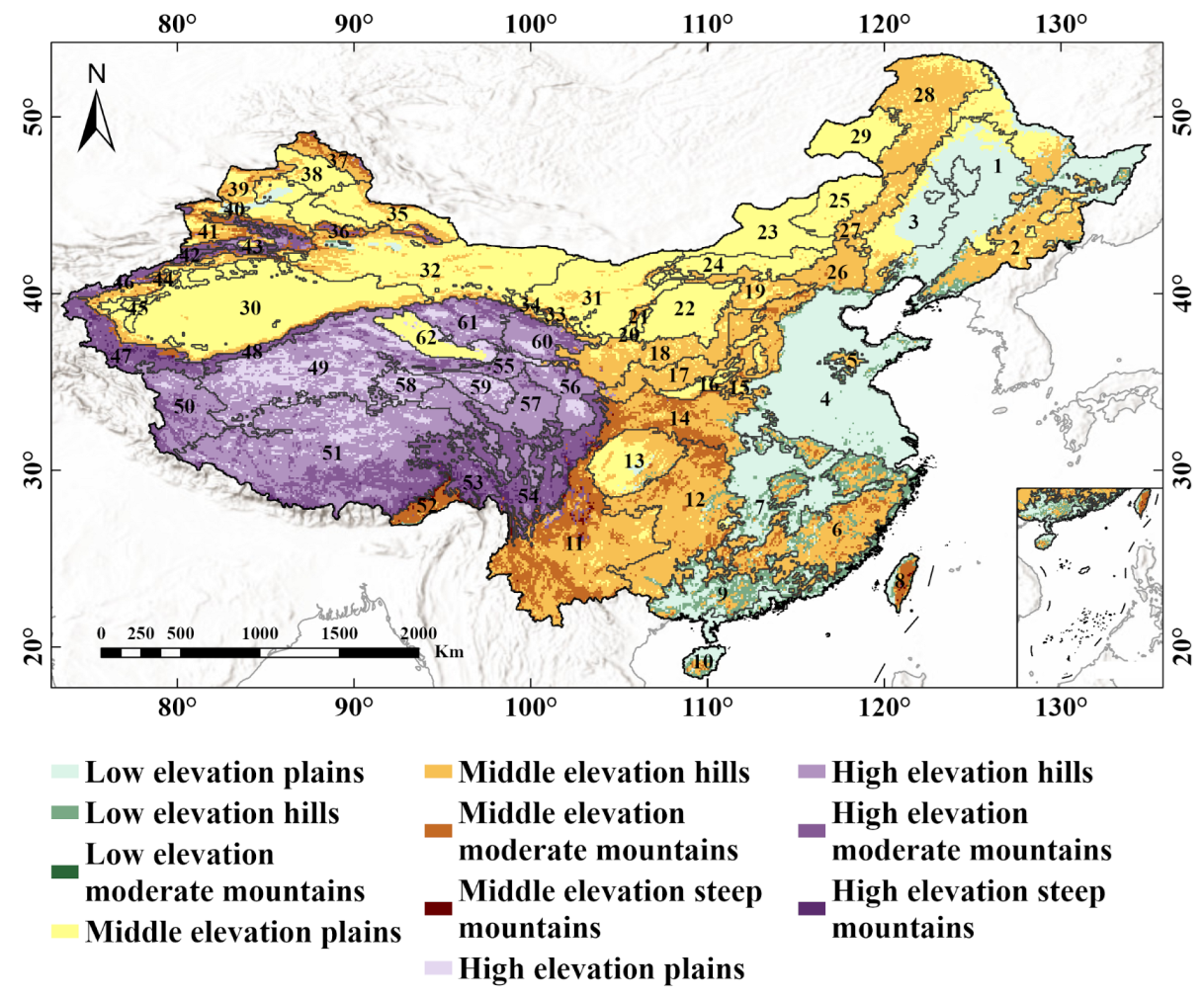
For the first step, the average elevation and topographic relief are appropriate for describing the correlation between the LST and landform on the AMSR2 pixel scale [29]. The average elevation affects the variation of the temperature in the vertical direction, while the topographic relief reflects the undulation of the terrain and affects the distribution of the temperature and its influence on the surroundings. These two parameters in the extent of AMSR2 pixel are calculated using the mean value and the value range of the SRTM pixels inside one AMSR2 pixel, respectively. A basic landform classification is obtained by overlapping the reclassified average elevation and topographic relief. Although there have been several different classification strategies for the basic landform types of China [42,43], they are basically the same on the scale of the AMSR2 pixel. A classification strategy identical to that in Zhang and Cheng [29] is adopted, with which 11 landform types are finally obtained (Figure A1). These landform types are assumed to be constant in the spatial scale of the AMSR2 pixel for the long-term.
For the second step, the MODIS LC product (MCD12Q1) with a classification accuracy of 75% used for AMSR-E [29] is replaced by the glacier-updated GlobeLand30 LC data. The MCD12Q1 data misclassified some LC types, particularly in the transition zones between the bareland and vegetation in Northwest China, while the GlobeLand30 data eliminated this problem significantly. As mentioned in Section 2.2.1, the annual GlobeLand30 dataset closest to the current year of AMSR2 was used to establish the CCSEV. These new LC data is first projected and resampled to match the basic landform type data. As counted from the GlobeLand30 data, there are nine different LC types in China (Figure A2), in which the vegetation associated (cultivated land, forest, grass land, shrubland) and barren LC types reaches 97.2%. Therefore, these two groups of LCs and the basic landform are separately overlaid to establish the landform, vegetated, and barren land classification system. It has been proven that landform impacts the distribution of the LST more than vegetation in the areas with large topographic fluctuations [29], so that merging the vegetated LC zones has little impact on the accuracy of the regression models in these fluctuating topographies (e.g., the zones in Southwestern China). Moreover, the overlaying of basic landform and vegetated and barren LCs generates plenty of scattered, small sliver polygons that lack samples for model regression. These polygons are merged into their surrounding large-size zones (widely spread in most zones). Some zones, especially in Northwest China, that are dominated with relatively flat terrain and bareland type, extend huge areas based on the current classification system. However, the deserts, which are mainly distributed in Northwest China and have distinct heat properties compared with the other LCs, are classified as bareland in the Globeland30 product. These zones are therefore divided into smaller zones according to the dataset of desert distribution in China. After the post-merging and dividing process, the classification system of landform and vegetated and barren land contains 62 zones (Figure 3).
For the third step, the other LC types taking up relatively small areas are introduced into the CCSEV, including wetland, waterbody, glacier, artificial, desert, and snow. The wetland is merged with waterbody due to their similarity. Desert is separated out using the dataset of deserts in China. The extent of snow cover changes every day and replaces the original LC, so it is necessary to include snow cover in the CCSEV. The regression models of most of the other LCs are not established according to the classification system in the second step due to their small areas. The 62 zones are therefore grouped into eight larger regions based on the landform and climate, as Figure 3 shows. The regression model for water, glacier, and artificial types are established according to the eight regions. The deserts in China are basically distributed as eight continuous large parts, according to which the regression models for deserts are established. Snow cover is unevenly spread in China. The western part and the eastern part of Northeast China and the QTP are the regions extensively covered by snow in cold months, while the other parts are scattered with snow infrequently. Therefore, the regression models for Northeast China and the QTP are established according to the 62 zones, while the regression models for other parts are established according to the eight regions. With the exception of the daily changing snow cover, the other LCs are considered to be varied throughout the annual cycle.
By upscaling the LC data to the spatial scale of the AMSR2 data, the problem of mixed pixels arises. An assumption is put forward to facilitate the LST retrieval; that is, that an AMSR2 pixel will be treated as ‘pure’ in case any LC type takes up over 60% of the pixel area, otherwise it is mixed.
For the fourth step, the day–night cycle and monthly intervals are introduced for the classification in the temporal scale. Seasonal or long-term intervals have generally been applied for establishing the regression model in previous studies. However, it has been proven that using monthly intervals is more reasonable in the context of China [29] due to its complex and various landscapes. Seasonal or long-term intervals ignore the huge climate diversities. For example, the seasons are divided into spring, summer, autumn, and winter in most regions of China, but the duration of each season varies spatially. The cold seasons last longer in northern or high-altitude regions, and shorter in southern or low-altitude regions. The use of monthly intervals overcomes this problem. Finally, the CCSEV for each year can be established according to the above steps.

3.3. Data Processing and Model Construction

Some data processing is necessary ahead of constructing the regression models, mainly including the quality control of the AMSR2 data and the upscaling of the MODIS LST. There is no quality screening data for the AMSR2 BT dataset; therefore, the abnormal values are removed using two indices, i.e., the polarization ratio (PR) used in Zhang and Cheng [29] and the newly introduced BT value thresholds. The pixels with an illogical PR value [44]—i.e., the polarized BT ratio of horizontal to vertical at the identical frequency greater than 1—are first removed, and the pixels with a horizontal BT greater than 310 K, vertical BT greater than 300 K, and non-water area BT less than 180 K at all channels are then removed. The MODIS LST are upscaled to the pixel size of the AMSR2 BT data before constructing the regression model; however, the topographic effect cannot be ignored because fluctuating topographies account for a large proportion of the area in China. The LST upscaling model proposed by Liu et al. [45], which considers the heat reflection of adjacent pixels, is applied in this study. To ensure the representativeness, only the upscaled MODIS LST pixels with a proportion of available pixels more than 60% are retained.
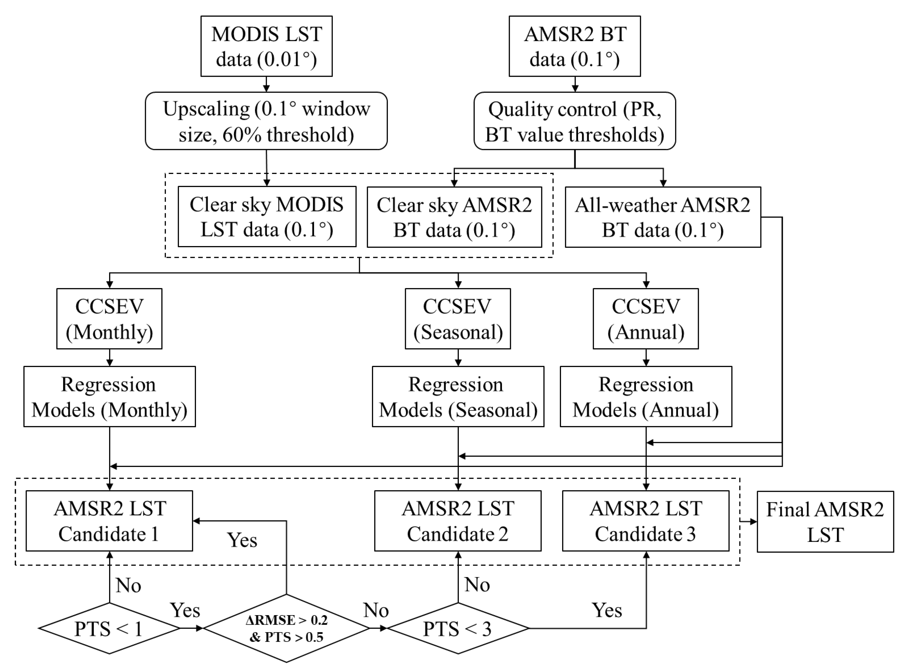
After the data processing, the regression models for all of the classes in the CCSEVs in terms of the years 2012 to 2020 are constructed (Figure 4). Some classes may have insufficient samples for model training due to cloud contamination, data quality control, and class dimension; the CCSEVs that replaced the monthly interval with seasonal intervals and annual intervals are therefore constructed as alternatives. To implement the replacement, two indices, i.e., the proportion of training samples (PTS) and RMSE, are introduced. The PTS indicates the ratio between the number of available pixels in a class (Na) and the number of pixels that this class covers in space (Nc). The RMSE is calculated between the retrieved AMSR2 LST and the reference MODIS LST.
P T S = N a / N c
R M S E = 1 n i = 1 n x i y i 2
where n is the sample number of LST pixels, x i is the value of the AMSR2 LST at pixel i, and y i is the value of the MODIS LST at pixel i. If the PTS of the monthly class is less than 1, the model lacks representativeness and should be replaced with the corresponding seasonal model. If the PTS of the alternative seasonal model is still less than 3, replace it with the annual model. Considering that the replacement may significantly increase the RMSE due to the uneven temporal distribution of the samples, a restrictive condition is added. That is, if the growth of the RMSE is greater than 0.2 and the PTS of the monthly class is more than 0.5, cancel the replacement. For mixed pixels, the LST is calculated by adding up the area-weighted LST for every LC used.

4. Results

4.1. Performance of the AMSR2 LST Retrieval Algorithm

The PTS and RMSE are used to assess the performance of the regression models for deriving the AMSR2 LST. The PTS measures the representativeness, while the RMSE reflects the accuracy. Figure 5 presents the monthly and day–night statistics for these two indices through boxplots, taking 2017 as an example. The boxplots reflect the distribution of the PTS and RMSE for the zones of landform and LC. For the sake of comparison, the mean values for daytime and nighttime are both displayed in the daytime and nighttime boxplots.
As seen in Figure 5a, there are only four months with a PTS less than 1 (illustrated by the position of bottom cap line) in the daytime and nighttime, respectively. Moreover, the quantity of classes with a PTS value less than 1 is quite small in these months, taking up only 1.1% to 2.3% of the total class number. These statistics indicate that the regression models are representative for large masses of the classes. Both the daytimes and nighttimes of the winter months, including January and February, have the highest mean PTS—of over 15—among the whole year. The daytime mean PTSs in different months are nearly all lower than those in the nighttime, with an average of 1.46, except December. These phenomena can be explained by the generally larger cloud cover in non-winter months and daytime in China.
Compared with the other months, the mean RMSEs (Figure 5b) are higher in the spring and early summer months, including March, April, May, and June, for both daytime and nighttime, and are higher in the late autumn and early winter months, including October, November, and December, for nighttime, which indicates that the models are relatively low in accuracy in these months. The mean RMSEs in the daytime range between 2.42 and 3.85 K for all 12 months, which are higher than those in the nighttime, which range between 2.29 and 2.68 K. That is, the fluctuation in the mean RMSE in the daytime throughout the year is higher than that in the nighttime. In the daytime for all months, the RMSEs for different classes is generally spread over a larger range compared with those in the nighttime, showing larger cap ranges in the daytime than those in the nighttime for all months expect February. The cap range varies between 3.14 and 5.48 K in the daytime, and 2.76 and 4.36 K in the nighttime. Combined with the daytime and nighttime variation in the PTS among different months, the opposite trend in the PTS and RMSE in March, April, May, and June makes it clear that cloud cover is one of the sources of the error in the models.
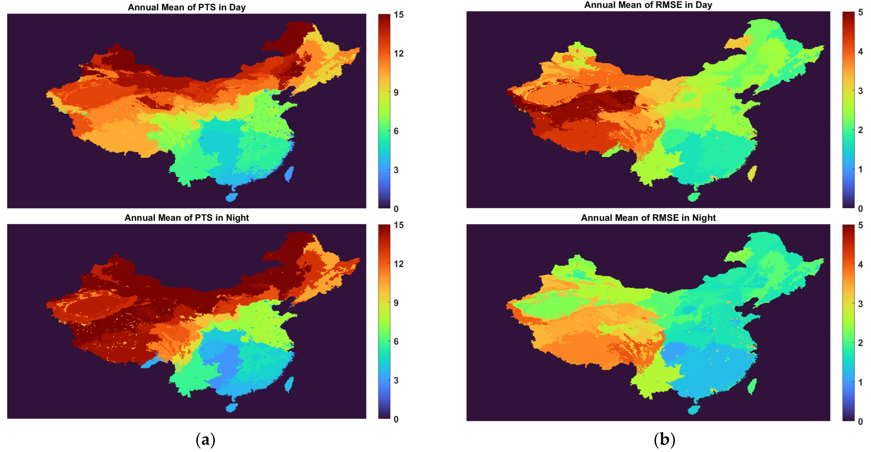
Figure 6 presents the spatial distribution of the mean PTSs and mean RMSEs in the zones of landform and LC in 2017. Similar to the situation in Figure 5a, the daytime PTSs of the zones across China are generally lower than those in the nighttime, and the daytime RMSEs are higher than those in the nighttime. In terms of space, both the daytime and nighttime zones in northern and western China have larger mean PTSs than those in central and southern China, meaning that the cloud cover is more frequent in the latter. The scattered ‘island’ zones of glacier, water, and artificial generally present explicitly different PTS values compared with the surrounding ‘ocean’ zones because of their huge area differences. The lowest mean PTSs for both daytime and nighttime occur in the artificial zone in Southwestern China, being 2.43 and 2.10, respectively. These values fall within the range defined as representative.
The mean RMSEs of the daytime zones are generally higher than those in the nighttime, consistent with the case in Figure 5b. In terms of space, the zones in western China have larger mean RMSEs than those in eastern China in both daytime and nighttime. It is notable that in the western China zones with higher PTSs, the RMSEs are also relatively large. Coupled with the effect of the significantly fluctuating topography, the RMSEs are relatively large in western China. In comparison, the RMSEs are small in the eastern China zones with lower PTSs; however, the PTSs are still in the range of representativeness. In the daytime, the western regions—including the QTP and the western part of Northwest China—have a larger overall mean RMSE of 3.78 K, while the remaining eastern regions have a lower overall mean RMSE of 2.44 K. In the nighttime, the western regions have a higher overall mean RMSE of 3.02 K, while the eastern regions have a lower overall mean RMSE of 1.88 K. The lowest and highest mean RMSEs appear in zone 9 and zone 47 in the daytime, being 1.64 K and 5.31 K, respectively, and in zone 13 and zone 53 in the nighttime, being 1.09 K and 4.06 K, respectively. These four zones are located in southern China, southwestern China, western QTP, and southeastern QTP, respectively.
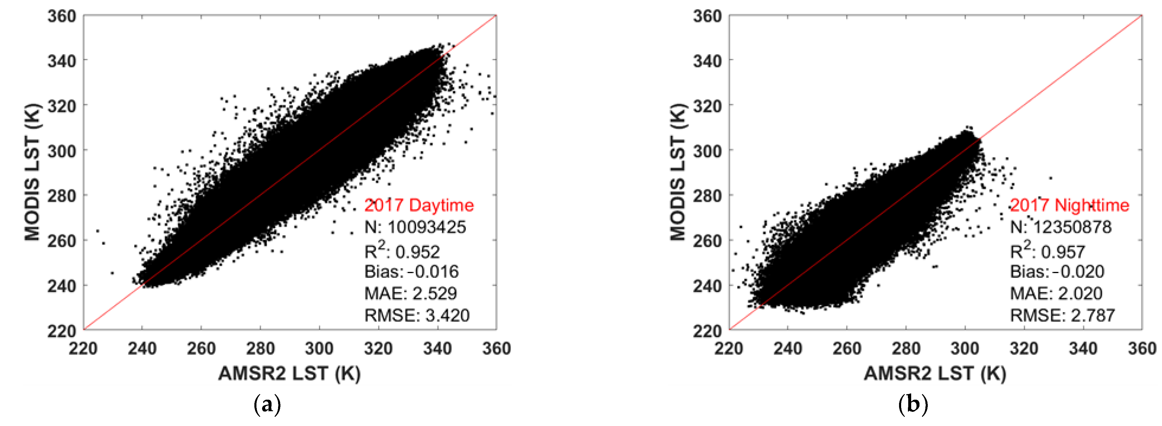
Figure 7 shows the verification of the daytime and nighttime AMSR2 LST in China with the MODIS LST in 2017. The R2 values are all higher than 0.95 and the bias values are all approximately −0.02 K, indicating that the proposed algorithm generally performs well. The RMSE of the AMSR2 LST is approximately 3.42 K in the daytime and 2.79 K in the nighttime, respectively.
The temporal and spatial distributions of the PTS and RMSE of the months and zones in the other years are very similar with those in 2017. Specifically, the quantity of zones with a PTS less than 1 is quite small between 2012 and 2020, taking up 0.1% to 2.0% of the number of classes for daytime or nighttime in each year. The annual mean PTSs range between 11.00 and 13.92 in the daytime and 12.07 to 15.39 in the nighttime in these years, except 2012, when the mean PTSs are 27.82 in the daytime and 30.81 in the nighttime because the retrieved AMSR2 LST are only available in the second half of the year. The daytime RMSEs in all months and zones in the other years are generally higher than those of the nighttime, and the RMSE showed an increasing trend in the spring and early summer months for both daytime and nighttime and an increasing trend in the late autumn and early winter months for nighttime. The annual mean RMSEs of the AMSR2 LST in China between 2012 and 2020 are listed in Table 1. It is not unexpected that the daytime RMSEs are higher than the nighttime RMSE in all of the years. The daytime RMSE ranges between 3.26 and 3.61 K, while the nighttime RMSE ranges between 2.76 and 2.96 K. In addition, the annual R2 of the AMSR2 and MODIS LSTs are all higher than 0.95 and up to 0.98 in these years.

4.2. Verification of AMSR2 LST with Field Observations

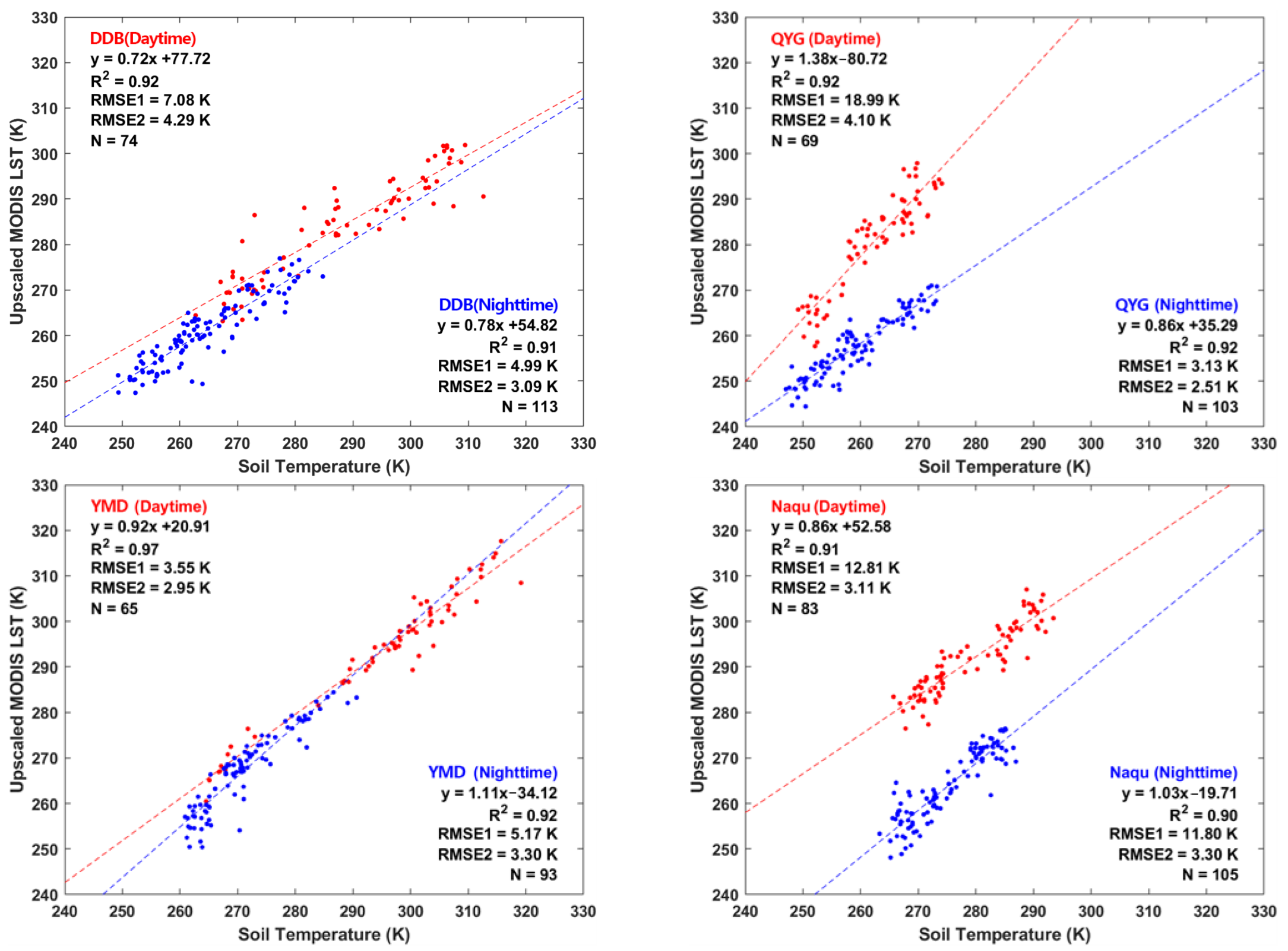
The comparison with the field observations can verify the accuracy of the AMSR2 LST in all-weather conditions. However, the field observations of the soil temperature and retrieved LST are different in terms of the spatial scale and physical definition. A commonly used method to weaken this influence is to calibrate the soil temperature by establishing a linear regression relationship with the reference LST at the AMSR2 LST pixel scale. This method is also applied in this study, in which the MODIS LST was treated as the reference and upscaled to the spatial resolution of the AMSR2 data before calibration. The DDB, QYG, and YMD sites in the BRB region provided the soil temperature observations from mid-August to December 2020, and the Naqu sites provided the observations from July to December 2012. The two sites in the Naqu region are inside one AMSR2 pixel, so the mean value of the soil temperature was used to fit the AMSR2 LST.
Figure 8 presents the calibration of the soil temperature for the verification sites in this study. The regression equation, R2, RMSE before calibration (RMSE1) and after calibration (RMSE2), and sample number (N) are also presented. It is noteworthy that the RMSE1 at the daytime QYG site (18.99 K) and both the daytime and nighttime Naqu sites (12.81 K and 11.80 K, respectively) are quite large due to the more heterogeneous landscape. In contrast, the RMSE1 in the other cases are relatively small because of the more homogeneous landscape. Nevertheless, the R2 for all sites is higher than 0.9 for both daytime and nighttime, which indicates that the soil temperature has a high correlation with the reference LST and the calibration of the field observations continues their variation trend but adjusts the values to the AMSR2 pixel scale. The RMSEs are therefore significantly decreased after calibration, especially in the daytime QYG (4.10 K) and the daytime and nighttime Naqu sites (3.10 K and 3.30 K, respectively).
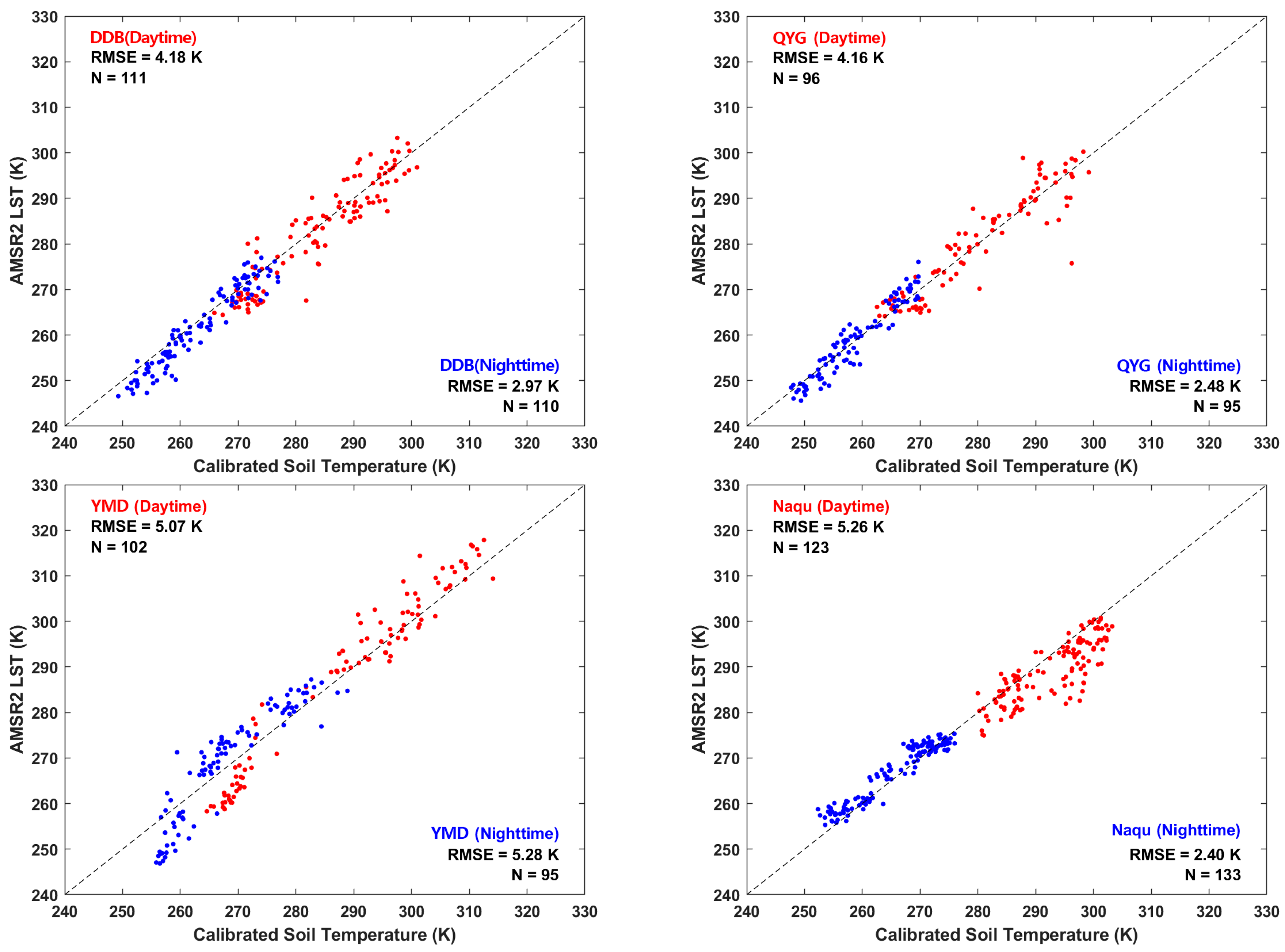
Figure 9 shows the verification of the AMSR2 LST with the calibrated soil temperature at the sites. The RMSEs of the AMSR2 LST at the DDB, QYG, YMD, and Naqu sites are 4.18 K, 4.16 K, 5.07 K, and 5.26 K in the daytime and 2.97 K, 2.48 K, 5.28 K, and 2.40 K in the nighttime, respectively. It is found that at the YMD site with bareland and flat topography, the RMSE of the AMSR2 LST is relatively high in both daytime and nighttime due to the strong penetrability of the MW signal into the arid surface. At the other sites, the RMSE of the retrieved AMSR2 LST is larger in the daytime, which confirms the pattern mentioned in Section 4.1.

4.3. The Spatiotemporal Variation of AMSR2 LST

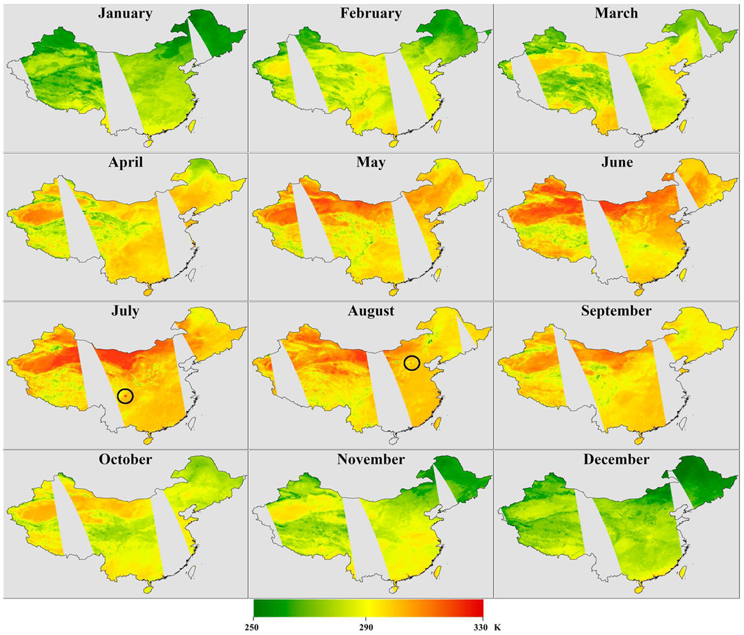
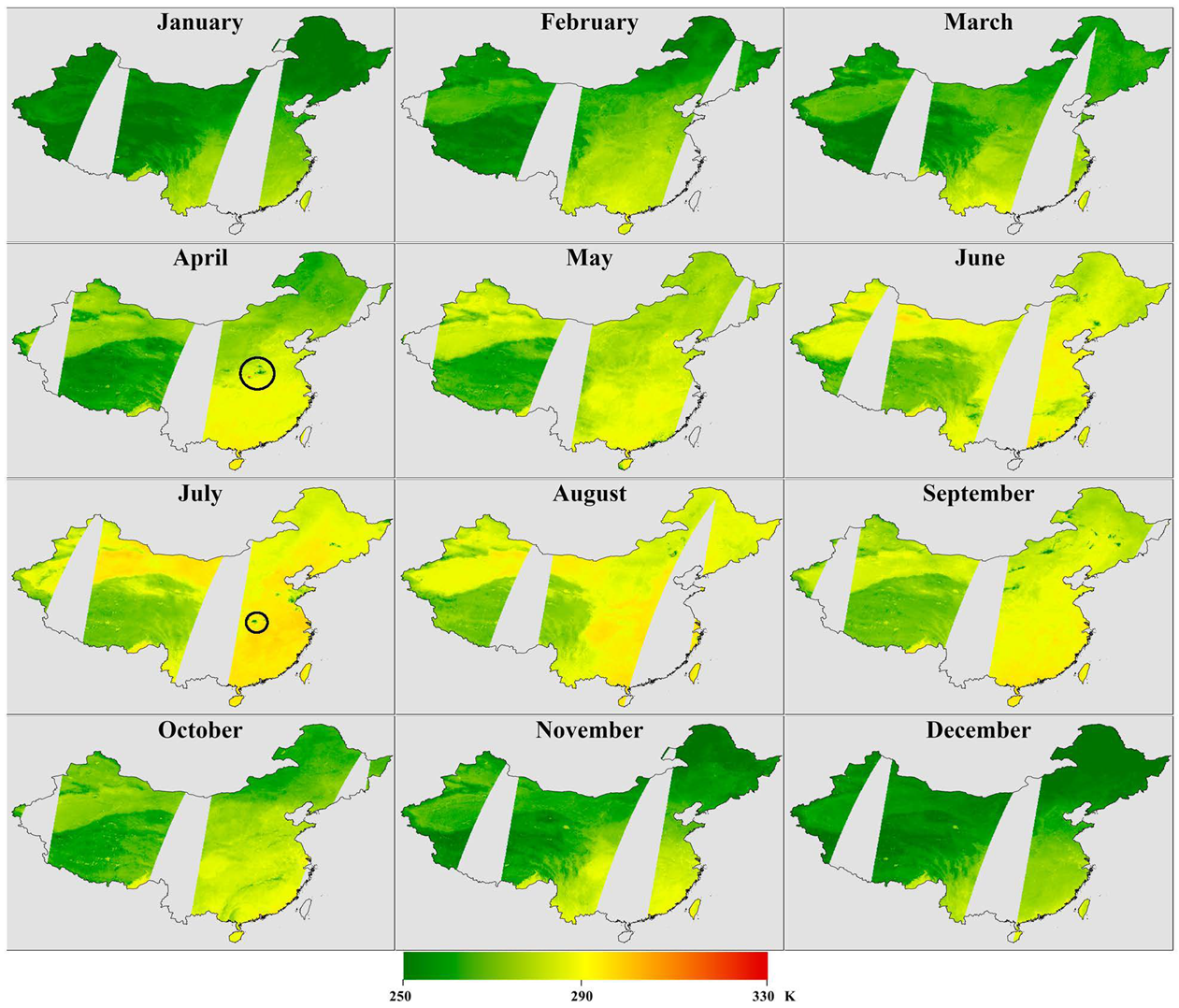
Figure 10 and Figure 11 present the AMSR2 LST images in China, taking the 15th day of every month during 2017 as an example. The gaps inside the extent of China are caused by the orbit of the AMSR2. These images correctly uncover the spatiotemporal distribution of the LST in China. In terms of time, the LST in both daytime and nighttime exhibits an overall trend of rising in the first half of the year and a trend of falling in the second half of the year. In terms of space, the QTP and Northeast China are two major regions controlled by a lower LST, while South China and the desert areas in northwestern China are controlled by a higher LST. However, some outliers still exist due to the incomplete data filter and algorithm design, shown via the black circles marked in Figure 10 and Figure 11. Therefore, the proposed algorithm for AMSR2 LST retrieval needs to be improved to remove these outliers.

5. Discussion

The performance of the algorithm is first assessed using two indicators—the PTS and the RMSE—in both the temporal scale and the spatial scale, in which the MODIS LST serves as the reference. Due to the optimization of the zones in the CCSEV, the quantity of classes with a PTS value less than 1 explicitly decreased from 10% to below 2% in the experimental years compared with that of the AMSR-E LST [29]. That is, more regression models are representative, which facilitates the performance of the optimized algorithm for AMSR2 LST retrieval. Although the comparison with the MODIS LST does not reflect the actual accuracy of the algorithm, the spatiotemporal variation in the performance of the algorithm can be evaluated using this method when other independent measurements of the LST are difficult to obtain continuously on a large spatial scale. In terms of time, the reason for the larger RMSE in the daytime and warm months is primarily solar radiation. The complex landscapes mean that the absorption of solar radiation and the emission of heat from the land surface vary greatly in the daytime and warm months, when the solar radiation is stronger. Consequently, the relationship between the BT and LST would also be very complicated. In terms of space, the reasons for the larger RMSEs in western China are mainly the LC and topography. Bareland and desert are the dominant LC types in arid western China, where the MW signal penetrates deeper layers below the surface. The terrain is also more fluctuating. Therefore, the distribution of the LST there is more complex. The regression models cannot represent the relationship between the BT and LST as well as that in eastern China, where the vegetation-related LCs dominate and the topography is relatively flat.
The locations for the zones with the lowest and highest mean RMSEs in the daytime and nighttime are very typical distributions of RMSE in accordance with the LC and landform, which further demonstrate the performance of the models under different landscapes. Zone 9, with the lowest mean RMSE in the daytime, is dominated by a relatively plain surface and cultivated land and forest. Zone 13, with the lowest mean RMSE in the nighttime, is dominated by quite weak fluctuating topography and cultivated land. Zone 47, with the highest mean RMSE in the daytime, is dominated by significantly fluctuating topography and bareland, grass land, and glacier. Zone 53, with the highest mean RMSE in the nighttime, is dominated by very fluctuating topography and bareland, grassland, and glacier.
Guided by the development of a more accurate product, the AMSR2 LST data in a certain experimental year are retrieved using the regression models constructed for their own year; therefore, the performance of the algorithm in different years is more stable than that for the AMSR-E LST [29], in which the regression models constructed by the training data of a specific year are applied in the retrieval of the LST in other years. The annual mean RMSEs of the AMSR2 LST in the experimental years are situated at 3.44 ± 0.18 K in the daytime and 2.86 ± 0.10 K in the nighttime, respectively. However, the annual mean RMSEs of the AMSR-E in non-training years decreased by 0.46 K in the daytime and 0.49 K in the nighttime, on average.
MODIS can only record the LST in clear sky conditions due to the nature of TIR sensors. As a key component making up the complete evaluation of the algorithm, the site measurements are introduced to evaluate the retrieved AMSR2 LST in all-weather conditions. In calibrating the soil temperature, the RMSE between the soil temperature and upscaled MODIS LST is quite large in some sites, including QYG and Naqu. In addition to the impact of the difference in the physical definition between these two types of temperatures, another important reason for large RMSEs lies in the scale effect. These sites are located in the mixed pixel of the AMSR2 scale, and the radiation features of various LCs in the pixel scale differ from each other greatly. The LC of the QYG site is snow and ice, while bareland and grassland occupy a large area inside the same pixel of the QYG site. The LC of the Naqu site is grassland, while water and bareland occupy a large area inside the same pixel of the Naqu sites. Moreover, the topography inside these two pixels is quite fluctuating, making the LST distribution complicated. In the daytime, the solar radiation enhances the unevenness of the temperature distribution. Although there are mixed pixels at the sites of DDB, QYG, and Naqu due to the varied LC types and fluctuating topography, the calibration of the soil temperature reduced the scale effect between the soil temperature and AMSR2 LST due to the higher R2, which results in a smaller RMSE after calibration at these sites, especially in the nighttime. Although the locations of the verification sites and the period of data in this study are different from those in previous studies, the accuracy of the retrieved AMSR2 LST in these studies [46] are equivalent in magnitude, being 4–5 K in the daytime and 2–4 K in the nighttime.

6. Conclusions

This study proposed an empirical algorithm to retrieve the AMSR2 LST. To ensure the continuity of the research of long-term series all-weather LST fusion, this algorithm was developed based on the algorithm in Zhang and Cheng [29], in which a CCSEV considering the combined influence of environmental variables was constructed for AMSR-E LST retrieval. The major modifications of the algorithm compared with that for AMSR-E LST retrieval were reflected in the optimization of the CCSEV establishment and model construction.
From the assessment of the AMSR2 LST retrieval algorithm, it can be concluded that: (1) The performance of the algorithm is mostly higher in the western China zones than in the eastern China zones, and generally higher in the daytime than in the nighttime; (2) The spatiotemporal distribution for the RMSE of the AMSR2 LST data is a consequence of the combined influence of cloud cover, solar radiation, LC, and topography; (3) The strong penetrability of the MW signal into the arid surface led to the relatively large RMSE in some sites (e.g., YMD) when verifying the AMSR2 LST through field observations.
The AMSR2 BT data has a higher resolution and more outliers compared with the AMSR-E BT data, which have been proven to have a negative effect on the accuracy of the retrieved LST data [47]; however, owing to the optimization of the algorithm, the AMSR2 LST retrieved in this study achieved comparable accuracy to that of the AMSR-E LST in Zhang and Cheng [29], in which the RMSE of the AMSR-E LST compared with the MODIS LST varies between 2.65 K and 3.48 K in the daytime and 2.08 K and 2.94 K in the nighttime in the years 2005 and 2009 to 2011. The comparable accuracy of these two datasets favors the all-weather LST fusion with the TIR LST and the analysis of a long-term series (since 2002) LST for climate research in China.
Although a retrieval algorithm with relatively high accuracy was developed, there are some defects in the retrieved AMSR2 LST that were not avoided. First, affected by the penetrability of the MW signal, the AMSR2 LST is actually the temperature at a certain depth below the land surface, and the depth is connected with the physical properties of the surface. This is why the accuracy of the AMSR2 LST in western China is lower. Second, the orbit gap takes up a large area of the extent of China, and the development of a filling algorithm is very critical but is not included in this study. Third, the outliers in the AMSR2 BT data were not fully removed using the PR and BT thresholds, resulting in some outliers in the final LST data. In addition, the AMSR2 LST is only verified at a few sites due to the lack of widespread field observations of the LST, which limits the reliability of the evaluation for the algorithm. This is a prevalent defect in the relevant research. To overcome this problem, the spatiotemporal continuous surface observations derived from the data assimilation system are developed by researchers (e.g., the daily soil temperature product at different depths provided by the China Meteorological Administration). Although the accuracy of this kind of dataset cannot catch up with the field observations at present, the constant improvement of their quality will make the verification of the satellite-derived LST data through these products more reliable in the future. Therefore, further efforts should be made to improve the accuracy of the AMSR2 LST by addressing these problems.

Author Contributions

Conceptualization, Q.Z. and N.W.; methodology, Q.Z.; validation, Q.Z. and Y.W.; formal analysis, Q.Z.; investigation, Q.Z. and Y.W.; resources, Q.Z., Y.W. and A.C.; data curation, Q.Z. and A.C.; writing—original draft preparation, Q.Z.; writing—review and editing, Q.Z., Y.W. and A.C.; visualization, Q.Z. and A.C.; supervision, Q.Z.; project administration, Q.Z. and N.W.; funding acquisition, Q.Z. and N.W. All authors have read and agreed to the published version of the manuscript.

Funding

This research was funded by the National Natural Science Foundation of China, grant number 42001293 and 42130516, and the Second Tibetan Plateau Scientific Expedition and Research Program, grant number 2019QZKK020102.

Data Availability Statement

The data presented in this study are available on request from the corresponding author. The data are not publicly available due to privacy.

Conflicts of Interest

The authors declare no conflict of interest. The funders had no role in the design of the study; in the collection, analyses, or interpretation of the data; in the writing of the manuscript; or in the decision to publish the results.

Abbreviations

AMSR2Advanced Microwave Scanning Radiometer 2
AMSR-EAdvanced Microwave Scanning Radiometer- Earth Observing System
BRBBeidahe River Basin
BTBrightness Temperature
CCSEVComprehensive Classification System of Environmental Variables
CTP-SMTMNCentral Tibet Plateau Soil Moisture and Temperature Monitoring Network
DDBDiaodabangou
ETM+Enhanced Thematic Mapper
LCLandcover
LSTLand Surface Temperature
MODISModerate Resolution Imaging Spectroradiometer
MWMicrowave
OLIOperational Land Imager
PRPolarization Ratio
PTSProportion of Training Samples
QTPQinghai-Tibet Plateau
QYGQiyi Glacier
RGI 6.0Randolph Glacier Inventory version 6.0
RMSERoot Mean Square Error
RTERadiation Transfer Equation
SCESnow-Cover-Extent
SRTMShuttle Radar Topography Mission
TM5Thematic Mapper 5
TIRThermal Infrared
YMDYumendong

Appendix A

The 62 zones and their spatial associations with the biogeographical division (based on landform and landcover) of China. Figure A1 and Figure A2 show the landform types and landcover types overlaying with the 62 zones, respectively. It is shown that most zones match the landform types or landcover types or both of them in boundary, while some zones have been adjusted according to the merging or dividing rules mentioned in Section 3.2. The adjustment of the zone boundaries ensures higher retrieval accuracy as much as possible.
Figure A1. The zones of landform, vegetated and bare land are numbered from 1 to 62 and overlay the basic landform types in China.
Remotesensing 15 03228 g0a1
Figure A2. The zones of landform, vegetated and bare land are numbered from 1 to 62 and overlay the landcover types in China.
Remotesensing 15 03228 g0a2

References

  1. Anderson, M.; Norman, J.; Kustas, W.; Houborg, R.; Starks, P.; Agam, N. A thermal-based remote sensing technique for routine mapping of land-surface carbon, water and energy fluxes from field to regional scales. Remote Sens. Environ. 2008, 112, 4227–4241. [Google Scholar] [CrossRef]
  2. Li, Z.; Tang, R.; Wan, Z.; Bi, Y.; Zhou, C.; Tang, B.; Yan, G.; Zhang, X. A review of current methodologies for regional evapotranspiration estimation from remotely sensed data. Sensors 2009, 9, 3801–3853. [Google Scholar] [CrossRef] [Green Version]
  3. Zhang, Y.; Cheng, J. Spatio-Temporal Analysis of Urban Heat Island Using Multisource Remote Sensing Data: A Case Study in Hangzhou, China. IEEE J. Sel. Top. Appl. Earth Obs. Remote Sens. 2019, 12, 3317–3326. [Google Scholar] [CrossRef]
  4. Zhou, J.; Chen, Y.; Wang, J.; Zhan, W. Maximum nighttime urban heat island (UHI) intensity simulation by integrating remotely sensed data and meteorological observations. IEEE J. Sel. Top. Appl. Earth Obs. Remote Sens. 2011, 4, 138–146. [Google Scholar] [CrossRef]
  5. Li, Z.-L.; Tang, B.-H.; Wu, H.; Ren, H.; Yan, G.; Wan, Z.; Trigo, I.F.; Sobrino, J.A. Satellite-derived land surface temperature: Current status and perspectives. Remote Sens. Environ. 2013, 131, 14–37. [Google Scholar] [CrossRef] [Green Version]
  6. Wang, L.; Koike, T.; Yang, K.; Yeh, P.J.-F. Assessment of a distributed biosphere hydrological model against streamflow and MODIS land surface temperature in the upper Tone River Basin. J. Hydrol. 2009, 377, 21–34. [Google Scholar] [CrossRef]
  7. Pu, R.; Bonafoni, S. Thermal infrared remote sensing data downscaling investigations: An overview on current status and perspectives. Remote Sens. Appl. Soc. Environ. 2023, 29, 100921. [Google Scholar] [CrossRef]
  8. Becker, F.; Li, Z.-L. Towards a local split window method over land surfaces. Int. J. Remote Sens. 1990, 11, 369–393. [Google Scholar] [CrossRef]
  9. Wan, Z.; Dozier, J. A generalized split-window algorithm for retrieving land-surface temperature from space. IEEE Trans. Geosci. Remote Sens. 1996, 34, 892–905. [Google Scholar] [CrossRef] [Green Version]
  10. Gillespie, A.R.; Rokugawa, S.; Matsunaga, T.; Cothern, J.S.; Hook, S.; Kahle, A.B. A temperature and emissivity separation from advanced spaceborne thermal emission and reflection radiometer (ASTER) images. IEEE Trans. Geosci. Remote Sens. 1998, 36, 1113–1126. [Google Scholar] [CrossRef]
  11. Yunyue, Y.; Privette, J.L.; Pinheiro, A.C. Analysis of the NPOESS VIIRS land surface temperature algorithm using MODIS data. IEEE Trans. Geosci. Remote Sens. 2005, 43, 2340–2350. [Google Scholar] [CrossRef]
  12. Sekertekin, A.; Bonafoni, S. Land Surface Temperature Retrieval from Landsat 5, 7, and 8 over Rural Areas: Assessment of Different Retrieval Algorithms and Emissivity Models and Toolbox Implementation. Remote Sens. 2020, 12, 294. [Google Scholar] [CrossRef] [Green Version]
  13. Duan, S.-B.; Li, Z.-L.; Leng, P. A framework for the retrieval of all-weather land surface temperature at a high spatial resolution from polar-orbiting thermal infrared and passive microwave data. Remote Sens. Environ. 2017, 195, 107–117. [Google Scholar] [CrossRef]
  14. Jang, K.; Kang, S.; Kimball, J.; Hong, S. Retrievals of All-Weather Daily Air Temperature Using MODIS and AMSR-E Data. Remote Sens. 2014, 6, 8387–8404. [Google Scholar] [CrossRef] [Green Version]
  15. Kou, X.; Jiang, L.; Bo, Y.; Yan, S.; Chai, L. Estimation of land surface temperature through blending MODIS and AMSR-E data with the Bayesian maximum entropy method. Remote Sens. 2016, 8, 105. [Google Scholar] [CrossRef] [Green Version]
  16. Shwetha, H.R.; Kumar, D.N. Prediction of high spatio-temporal resolution land surface temperature under cloudy conditions using microwave vegetation index and ANN. Isprs J. Photogramm. Remote Sens. 2016, 117, 40–55. [Google Scholar] [CrossRef]
  17. Wang, T.; Shi, J.; Yan, G.; Zhao, T.; Ji, D.; Xiong, C. Recovering land surface temperature under cloudy skies for potentially deriving surface emitted longwave radiation by fusing MODIS and AMSR-E measurements. In Proceedings of the Geoscience and Remote Sensing Symposium (IGARSS), 2014 IEEE International, Quebec City, QC, Canada, 13–18 July 2014; pp. 1805–1808. [Google Scholar]
  18. Zhang, Q.; Cheng, J.; Wang, N. Fusion of All-Weather Land Surface Temperature from AMSR-E and MODIS Data Using Random Forest Regression. IEEE Geosci. Remote Sens. Lett. 2022, 19, 2502705. [Google Scholar] [CrossRef]
  19. Njoku, E.G.; Li, L. Retrieval of land surface parameters using passive microwave measurements at 6–18 GHz. IEEE Trans. Geosci. Remote Sens. 1999, 37, 79–93. [Google Scholar] [CrossRef] [Green Version]
  20. McFarland, M.J.; Miller, R.L.; Neale, C.M. Land surface temperature derived from the SSM/I passive microwave brightness temperatures. IEEE Trans. Geosci. Remote Sens. 1990, 28, 839–845. [Google Scholar] [CrossRef]
  21. Pulliainen, J.T.; Grandell, J.; Hallikainen, M.T. Retrieval of surface temperature in boreal forest zone from SSM/I data. IEEE Trans. Geosci. Remote Sens. 1997, 35, 1188–1200. [Google Scholar] [CrossRef]
  22. Wen, J.; Su, Z.; Ma, Y. Determination of land surface temperature and soil moisture from Tropical Rainfall Measuring Mission/Microwave Imager remote sensing data. J. Geophys. Res. Atmos. 2003, 108, ACL 2-1–ACL 2-10. [Google Scholar] [CrossRef] [Green Version]
  23. Zhou, J.; Dai, F.; Zhang, X.; Zhao, S.; Li, M. Developing a temporally land cover-based look-up table (TL-LUT) method for estimating land surface temperature based on AMSR-E data over the Chinese landmass. Int. J. Appl. Earth Obs. Geoinf. 2015, 34, 35–50. [Google Scholar] [CrossRef]
  24. Huang, C.; Duan, S.-B.; Jiang, X.-G.; Han, X.-J.; Leng, P.; Gao, M.-F.; Li, Z.-L. A physically based algorithm for retrieving land surface temperature under cloudy conditions from AMSR2 passive microwave measurements. Int. J. Remote Sens. 2019, 40, 1828–1843. [Google Scholar] [CrossRef]
  25. Holmes, T.; De Jeu, R.; Owe, M.; Dolman, A. Land surface temperature from Ka band (37 GHz) passive microwave observations. J. Geophys. Res. Atmos. 2009, 114, D04113. [Google Scholar] [CrossRef] [Green Version]
  26. Owe, M.; Van De Griend, A. On the relationship between thermodynamic surface temperature and high-frequency (37 GHz) vertically polarized brightness temperature under semi-arid conditions. Int. J. Remote Sens. 2001, 22, 3521–3532. [Google Scholar] [CrossRef]
  27. Mao, K.B.; Shi, J.C.; Li, Z.L.; Qin, Z.H.; Li, M.C.; Xu, B. A physics-based statistical algorithm for retrieving land surface temperature from AMSR-E passive microwave data. Sci. China Ser. D Earth Sci. 2007, 50, 1115–1120. [Google Scholar] [CrossRef]
  28. Hollinger, J. DMSP Special Sensor Microwave/Imager Calibration/Validation; Naval Research Lab: Washington, DC, USA, 1991. [Google Scholar]
  29. Zhang, Q.; Cheng, J. An Empirical Algorithm for Retrieving Land Surface Temperature from AMSR-E Data Considering the Comprehensive Effects of Environmental Variables. Earth Space Sci. 2020, 7, e2019EA001006. [Google Scholar] [CrossRef] [Green Version]
  30. Friedl, M.A.; Sulla-Menashe, D.; Tan, B.; Schneider, A.; Ramankutty, N.; Sibley, A.; Huang, X. MODIS Collection 5 global land cover: Algorithm refinements and characterization of new datasets. Remote Sens. Environ. 2010, 114, 168–182. [Google Scholar] [CrossRef]
  31. Hao, X. A New MODIS Snow Cover Extent Product over China (2000–2020); National Tibetan Plateau Data Center: Lanzhou, China, 2021. [Google Scholar] [CrossRef]
  32. Chen, J.; Ban, Y.; Li, S. Open access to Earth land-cover map. Nature 2014, 514, 434. [Google Scholar] [CrossRef] [Green Version]
  33. Kottek, M.; Grieser, J.; Beck, C.; Rudolf, B.; Rubel, F. World map of the Koppen-Geiger climate classification updated. Meteorol. Z. 2006, 15, 259–263. [Google Scholar] [CrossRef]
  34. Wan, Z. New refinements and validation of the MODIS land-surface temperature/emissivity products. Remote Sens. Environ. 2008, 112, 59–74. [Google Scholar] [CrossRef]
  35. Hao, X.; Huang, G.; Zheng, Z.; Sun, X.; Ji, W.; Zhao, H.; Wang, J.; Li, H.; Wang, X. Development and validation of a new MODIS snow-cover-extent product over China. Hydrol. Earth Syst. Sci. 2021, 26, 1937–1952. [Google Scholar] [CrossRef]
  36. Zhang, Q.; Yang, Q.; Wang, C. SRTM Error Distribution and its Associations with Landscapes across China. Photogramm. Eng. Remote Sens. 2016, 82, 135–148. [Google Scholar] [CrossRef]
  37. Zandbergen, P. Applications of shuttle radar topography mission elevation data. Geogr. Compass 2008, 2, 1404–1431. [Google Scholar] [CrossRef]
  38. Yang, L.; Meng, X.; Zhang, X. SRTM DEM and its application advances. Int. J. Remote Sens. 2011, 32, 3875–3896. [Google Scholar] [CrossRef]
  39. LIGGD. The Map of Desert Distribution in 1:2,000,000 in China; Chung-Hwa Publisher: Shanghai, China, 1974. [Google Scholar]
  40. RGI Consortium. Randolph Glacier Inventory—A Dataset of Global Glacier Outlines: Version 6.0; NSIDC: National Snow and Ice Data Center: Boulder, CO, USA, 2017. [Google Scholar]
  41. Sun, D.; Pinker, R.T. Estimation of land surface temperature from a Geostationary Operational Environmental Satellite (GOES-8). J. Geophys. Res. Atmos. 2003, 108, 4326. [Google Scholar] [CrossRef]
  42. Li, B.; Pan, B.; Cheng, W.; Han, J.; Qi, D.; Zhu, C. Research on geomorphological regionalization of China. Acta Geogr. Sin. 2013, 68, 291–306. [Google Scholar] [CrossRef]
  43. Zhou, C.; Cheng, W.; Qian, J.; Li, B.; Zhang, B. Research on the Classification System of Digital Land Geomorphology of 1:1,000,000 in China. J. Geo-Inf. Sci. 2009, 11, 707–724. [Google Scholar] [CrossRef]
  44. Gao, H.; Fu, R.; Dickinson, R.E.; Juárez, R.I.N. A practical method for retrieving land surface temperature from AMSR-E over the amazon forest. IEEE Trans. Geosci. Remote Sens. 2008, 46, 193–199. [Google Scholar] [CrossRef]
  45. Liu, Y.; Hiyama, T.; Yamaguchi, Y. Scaling of land surface temperature using satellite data: A case examination on ASTER and MODIS products over a heterogeneous terrain area. Remote Sens. Environ. 2006, 105, 115–128. [Google Scholar] [CrossRef]
  46. Lian, Y.; Duan, S.B.; Huang, C.; Han, W.; Liu, M. Generation of Spatial-Seamless AMSR2 Land Surface Temperature in China During 2012–2020 Using a Deep Neural Network. IEEE Trans. Geosci. Remote Sens. 2023, 61, 1–18. [Google Scholar] [CrossRef]
  47. Ghosh, A.; Joshi, P.K. Hyperspectral imagery for disaggregation of land surface temperature with selected regression algorithms over different land use land cover scenes. ISPRS J. Photogramm. Remote Sens. 2014, 96, 76–93. [Google Scholar] [CrossRef]
Figure 1. The study area and verification regions. The green dots indicate the verification sites.
Remotesensing 15 03228 g001
Figure 2. The flow chart for establishing the CCSEV involving four steps.
Remotesensing 15 03228 g002
Figure 3. The zones of landform, vegetated and bare land numbered from 1 to 62. These zones are categorized into eight major regions by color. The LC types of desert, artificial, water and glacier are also presented.
Remotesensing 15 03228 g003
Figure 4. The flow chart for training the regression model and retrieving AMSR2 LST.
Remotesensing 15 03228 g004
Figure 5. The monthly and day-night statistics of (a) PTS and (b) RMSE for the regression models.
Remotesensing 15 03228 g005
Figure 6. The spatial and day-night statistics of (a) PTS and (b) RMSE for the regression models.
Remotesensing 15 03228 g006
Figure 7. The verification of AMSR2 LST in China with reference MODIS LST in (a) daytime and (b) nighttime of 2017.
Remotesensing 15 03228 g007
Figure 8. The calibration of soil temperature at the verification sites in both daytime and nighttime.
Remotesensing 15 03228 g008
Figure 9. The verification of AMSR2 LST with the calibrated soil temperature at the sites in both daytime and nighttime.
Remotesensing 15 03228 g009
Figure 10. The images of daytime AMSR2 LST in China on the monthly example day during 2017.
Remotesensing 15 03228 g010
Figure 11. The images of nighttime AMSR2 LST in China on the monthly example day during 2017.
Remotesensing 15 03228 g011
Table 1. The annual mean RMSEs of AMSR2 LST in China from 2012 to 2020 for both daytime and nighttime.
Year201220132014201520162017201820192020
Daytime (K)3.2643.4563.5283.5613.6053.4203.5083.4443.589
Nighttime (K)2.7642.8012.8332.8092.8392.7872.8152.7562.956
Disclaimer/Publisher’s Note: The statements, opinions and data contained in all publications are solely those of the individual author(s) and contributor(s) and not of MDPI and/or the editor(s). MDPI and/or the editor(s) disclaim responsibility for any injury to people or property resulting from any ideas, methods, instructions or products referred to in the content.