Abstract
Spectral unmixing (SU) is a significant preprocessing task for handling hyperspectral images (HSI), but its process is affected by nonlinearity and spectral variability (SV). Currently, SV is considered within the framework of linear mixing models (LMM), which ignores the nonlinear effects in the scene. To address that issue, we consider the effects of SV on SU while investigating the nonlinear effects of hyperspectral images. Furthermore, an augmented generalized bilinear model is proposed to address spectral variability (abbreviated AGBM-SV). First, AGBM-SV adopts a generalized bilinear model (GBM) as the basic framework to address the nonlinear effects caused by second-order scattering. Secondly, scaling factors and spectral variability dictionaries are introduced to model the variability issues caused by the illumination conditions, material intrinsic variability, and other environmental factors. Then, a data-driven learning strategy is employed to set sparse and orthogonal bases for the abundance and spectral variability dictionaries according to the distribution characteristics of real materials. Finally, the alternating direction method of multipliers (ADMM) optimization method is used to split and solve the objective function, enabling the AGBM-SV algorithm to estimate the abundance and learn the spectral variability dictionary more effectively. The experimental results demonstrate the comparative superiority of the AGBM-SV method in both qualitative and quantitative perspectives, which can effectively solve the problem of spectral variability in nonlinear mixing scenes and to improve unmixing accuracy.
1. Introduction
Hyperspectral images (HSI) contain a large amount of spectral band information, which is collected by specific spectral sensors in hundreds of narrow and contiguous spectral bands. These bands correspond to wavelengths that span the visible range (VIS) and near-infrared range (NIR). HSI can support various types of remote sensing applications [1], such as classification [2], fusion [3], target detection [4], etc. However, the acquisition process of HSI may be affected by low spatial resolution or sensor accuracy, resulting in the mixture of multiple materials in some pixels. These so-called mixed pixels make the interpretation of hyperspectral data more difficult and affect the applications of hyperspectral imaging [5].
Spectral unmixing (SU) aims to determine the composition materials (endmembers) and their proportion (abundance fractions) in each pixel. Due to its importance for data interpretation and analysis, SU has become one of the main topics in hyperspectral data analysis. In most spectral unmixing applications, the linear mixing model (LMM) is assumed [6]. However, in actual observational scenes, nonlinear and spectral variability problems can occur and can seriously affect the accuracy of unmixing algorithms. For example, in vegetation-covered areas and complex urban scenes, there are nonlinear effects caused by multiple reflections between endmembers, i.e., materials that are spectrally unique in the wavelength bands used to collect the image [7,8]. There is also spectral variability due to illumination conditions, atmospheric effects and intrinsic variability in the properties of the pure material [9,10,11,12]. This indicates that it is not sufficient to simply generalize the use of linear models and that spectral variability must also be taken into consideration. Therefore, it is important to incorporate the spectral variability that occurs in practical scenarios into nonlinear spectral unmixing algorithms, which will have significant implications for practical applications.
In order to address the nonlinear effects caused by multiple layers of reflection from different endmembers, a kernel function approach has been proposed [13]. The idea of the kernel function approach is to transform the original nonlinear data into a higher-dimensional space, and then apply a linear unmixing method to solve the problem. However, this strategy is prone to becoming trapped in local minima and can lead to a poor unmixing performance. There are also some high-order mixing models that consider second-order or higher-order interactions, such as multilinear mixing models [14], p-linear models [15], and multi-harmonic post-nonlinear mixing models [16]. However, interactions beyond the second order incur a heavy computational cost. To overcome that, a classical and efficient method based on physical models is the use of a generalized bilinear model (GBM) [17]. GBM can effectively handle the assumptions in bilinear mixing models (BMM) [18,19] and is considered to be a generalization of LMM and FM [8,20].
Although GBM can effectively solve the nonlinearity caused by multiple scattering, it does not take into account the spectral variability in nonlinear scenarios. In some research papers, several theoretical models have been proposed to simulate spectral variability. However, most of these were implemented using the LMM framework. For example, the ELMM algorithm in [21] solves the spectral variability problem caused by illumination factors by scaling and adding proportional factors to each endmember in each pixel. The PLMM proposed in [22] explains variability by adding additive perturbations to endmembers, which often leads to significant errors. For example, scaling factors, as the primary source of spectral variability, should align with the spectral signatures of endmembers, while other variabilities often exhibit inconsistencies with the spectral signatures. Therefore, explaining spectral variability through simple additional terms is not effective. Similarly, the superpixel-based multi-scale transform extended linear model [23] resolves spectral variability using spatial information from HSI. This is a relatively fast processing algorithm, but it lacks accuracy in unmixing. In [24], a strategy is proposed to consider both nonlinear effects and spectral variability. The idea is to introduce intra-class variability of materials into the quadratic linear model, and then add extended constraint conditions from non-negative matrix factorization to the linear quadratic model for optimization. However, experimental results show that it does not give better abundance estimation results compared with results of experiments when only endmember variability is considered.
To address the nonlinearity and spectral variability issues in hyperspectral imaging, here we consider spectral variability fully in the proposed nonlinear unmixing model. We propose an augmented generalized bilinear model to address spectral variability in hyperspectral unmixing, called AGBM-SV. Specifically, the main contributions of this work can be summarized as follows:
(1) The proposed AGBM-SV algorithm introduces scaling factors and a spectral variability dictionary into the GBM nonlinear model, which can consider the spectral variability caused by various factors fully in the nonlinear model and alleviate the adverse effects of spectral variability on abundance estimation.
(2) The proposed AGBM-SV algorithm adopts a data-driven strategy, setting sparse constraints on the abundance matrix based on the distribution characteristics of real materials. Simultaneously, it specifies a spectral variability dictionary composed of orthogonal bases between low-coherent endmembers.
(3) The AGBM-SV algorithm employs an optimization method based on the alternating direction method of multipliers (ADMM), which decomposes the AGBM-SV objective function into small sub-problems that can be solved efficiently.
The rest of the paper is organized as follows. Section 2 reviews related works along with their advantages and disadvantages. It then describes the detailed steps of the proposed AGBM-SV method and the corresponding ADMM optimization process. Section 3 presents experimental results conducted on synthetic and real datasets, accompanied by qualitative and intuitive analyses. Finally, Section 4 presents conclusions and suggests directions for future research.
2. Materials and Methods
2.1. The Related GBM
In the LMM, each pixel can be written as follows:
where represents an L × R matrix containing R pure spectral features (endmembers), represents the R × 1 vector of the fractional abundance of the corresponding endmembers, and represents an L × 1 vector of noise errors for each spectral band. To satisfy the physical meaning of abundance, it is generally required that the abundance satisfy non-negativity constraints (ANC, ) and sum-to-one constraints (ASC, ).
The LMM may not always hold true in many situations [25]. However, GBM is an extended form of BMM and FM that solves non-linear phenomena through bilinear modeling and ignores the influence of high-order terms with low contributions. The expression of GBM mixed pixel matrix can be represented as:
where represents the endmember matrix, is the corresponding abundance matrix, represents the bilinear endmember interaction matrix, is the corresponding bilinear abundance matrix, is the nonlinear coefficient controlling the interaction between the and the endmembers in the pixel, and represents the noise term.
For the GBM expressed in Equation (3), the constraint can be summarized as:
where the matrix B is determined by the other matrices .
2.2. ALMM Addresses Spectral Variability
Inspired by the work in [26] on dealing with spectral variability, we propose here an augmented linear mixed model (ALMM). The ALMM extends the LMM by using a constant scale factor and an additive term defined as a dictionary of spectral variability. This approach theoretically allows the ALMM to learn the spectral variability adaptively in a data-driven learning process. Its model framework can be expressed as follows:
where is the spectral variability dictionary and D is the number of basis vectors in W. The expression represents the matrix of coefficients corresponding to W. is the diagonal matrix containing the scaling factors for all pixels with diagonal values of . Therefore, ALMM represents the spectral data as the sum of AXS scaled for each pixel and WH spectral variability dictionary, which allows ALMM to adaptively learn spectral variability in a data-driven learning process.
Although the ALMM algorithm is not able to handle the multiple reflections that occur in the observed scenes, leading to significant errors in estimating the endmember and abundance matrices, it reveals significant potential in describing spectral variability using scaling factors and spectral variability dictionaries. Therefore, for the proposed AGBM-SV model, we adopt a similar approach to deal with spectral variability.
2.3. The Proposed AGBM-SV Model Framework
To simultaneously address the nonlinearity in spectral unmixing and spectral variability, the augmented GBM nonlinear model to address spectral variability (AGBM-SV) algorithm is proposed. The AGBM-SV model consists of two main components: the scaled nonlinear module and the spectral variability module.
The scaled nonlinear module employs the GBM as the underlying framework to handle the nonlinear effects caused by multiple scattering. It also introduces shared scaling factors to address spectral variability resulting from illumination conditions and terrain factors. The spectral variability module consists of a spectral variability dictionary and corresponding coefficient matrix to handle other spectral variables and residual error terms. Figure 1 shows the overall structure of the proposed AGBM-SV unmixing model through the Cuprite dataset.
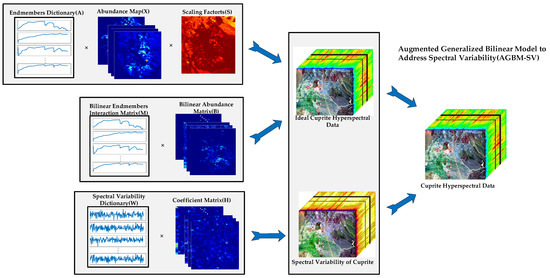
Figure 1.
The holistic diagram of the proposed AGBM-SV.
2.3.1. Scaled Nonlinear Module
Terrain and lighting conditions can affect the spectral reflectance of hyperspectral remote sensing images, resulting in changes in the proportion relationship between mixed pixels and endmembers. This may be caused by factors such as terrain shadow effects, variations in lighting direction, and intensity. To address these issues, scaling factors can be used to adjust the relationship between mixed pixels and endmembers, reflecting the influence of terrain and lighting conditions [26,27]. For example, in [28], it is assumed that all endmembers within a pixel are constant at the observation scale. Therefore, a shared scaling factor is used for each endmember in the linear term of the GBM. Each pixel can be represented as follows:
where represents a scalar for the i-th pixel, which can be simply estimated through regression between and . Therefore, for the mixed pixel matrix , the GBM model with the introduced scaling factor in Equation (2) can be represented as:
where is a diagonal matrix containing the scaling factors for all pixels, with diagonal values denoted as .
2.3.2. Spectral Variability Module
Although scaling factors can address some of the spectral variability caused by illumination conditions, factors such as intra-class spectral variability also fall within the scope of spectral variability. Moreover, using scaling factors alone may introduce some minor errors. To further overcome the difficulty of other spectral variables and error terms in the scaled nonlinear module, the freedom of the spectral variability dictionary [26] is added to the model to solve this problem. Adding degrees of freedom to correct for small induced residual errors is explained in detail in [29]. In this way, we simulate spectral variability and multiple scattering effects by adding a scaling factor and a spectral variability dictionary to the GBM. The proposed algorithm is called augmented GBM nonlinear models to address spectral variability (AGBM-SV). It can be written in the form with constraints as follows:
It is worth noting that the spectral variability dictionary is composed of orthogonal bases among low-coherent endmembers, which can better expand the variability dictionary and improve its generality. Overall, the AGBM-SV model is based on the perspective of nonlinear spectral unmixing and considers various types of spectral variability, such as illumination conditions, atmospheric environment, and the intrinsic variation of the spectral signatures of the materials. This improves the robustness of the model and the accuracy of unmixing.
2.4. Problem Formulation of AGBM-SV
The proposed AGBM-SV model to deal with complex spectral variability and non-linear effects can be formulated as the following constrained optimization problem:
where the goal is to estimate the variables X, S, B, W, and H, while the observed hyperspectral data Y and the endmember matrix X are given. For Equation (8), we assume that the endmembers matrix A is known. First, we estimate the number of endmembers in the image using HySime [30], and then use VCA [31] to extract the endmember matrix A. Because Equation (8) is an ill-posed problem, we made reasonable prior assumptions and introduced regular term. The three regularization terms are described below.
(1) Abundance matrix regularization : In reality, the mixed spectra are represented by the characteristic spectra of a limited number of materials, which are decomposed into a small number of endmember spectral feature sets and corresponding abundance information. Therefore, we set the abundance regularization as a sparse constraint. However, the norm of the abundance matrix is a non-convex optimization problem, so we replace it with the norm. The optimization process uses to approximate the sparse term, and the penalty parameter is represented by . Therefore, the matrix expression can be written as
(2) Spectral variability dictionary regularization : The spectral variability dictionary is designed to better explain the variability of materials within or between classes, which should not be attributed to the original materials, but rather to a new material or component. Therefore, the spectral variability dictionary should have low correlation with the endmember matrix (A). Additionally, the basis vectors in the spectral variability dictionary (W) may be orthogonal to fully represent various potential spectral features. Detailed explanations on this topic can be found in [26,32]. Therefore, the result expression for the regularization of W is:
where the first term represents the low correlation between the spectral variability dictionary (W) and the endmember matrix (A), while the second term represents the orthogonality of the basis vectors in W. and are the corresponding penalty parameters in the constraint conditions.
(3) Regularization of spectral variability coefficients : The spectral variability coefficients are generally determined by various factors in a given observation scenario. In the ELMM model, the scaling factor (S) can be obtained by modeling with the endmember dictionary, while the modeling process for other types of spectral variability coefficients and scaling factors is different. In order to enhance the reliability and generalization ability of the AGBM-SV model, the variability coefficients (H) of the spectral variability dictionary (W) are regularized with the Frobenius norm parameterized by :
Moreover, it should be noted that the constraints in Equation (8) must be satisfied. because the abundance matrix (X) and scaling factor (S) need to comply with the physical assumptions of reality, it is necessary to ensure that . Furthermore, for the nonlinear term in the abundance matrix B, it is required to satisfy . Because the variables X and S are bundled together in Equation (8), we use a relaxation technique to enforce the sum-to-one constraint on X. Through these constraints, the AGBM-SV model can better simulate nonlinear effects and spectral variations in real-world scenarios.
2.5. ADMM-Based Optimization Algorithm
The alternating direction method of multipliers (ADMM) algorithm is an iterative method for solving optimization problems [33,34,35]. The main steps of ADMM involve transforming the constrained optimization problem defined in Equation (8) into an unconstrained expression through augmented Lagrangian, and then iteratively minimizing the introduced auxiliary variables and Lagrange multipliers. Based on Equation (8), we need to solve for variables . Using the ADMM method for such multi-variable optimization problems can expand the solution space of variables, thus enabling us to obtain a better global minimum.
Although the objective function in Equation (8) is not simultaneously convex for all variables, it can be transformed into a convex optimization problem for each variable when the other variables are fixed. By introducing multiple auxiliary variables to replace and , and updating them alternately during optimization, the objective function can be minimized. The augmented Lagrangian function for Equation (8) can be written in the form of Equation (12):
where is the Lagrange multiplier and represents the penalty parameter. The overall process for solving Equation (12) is summarized in Algorithm 1, and Appendix A provides a detailed explanation of the solution process for each sub-problem. Algorithm 1 uses the classical multi-block ADMM optimization problem, which has been widely applied and proven to converge to solutions. In our experiments, we randomly selected blocks from three experimental datasets, and the convergence results for the corresponding datasets are visualized in Figure 2. For theoretical proofs and applications of the optimization problem, please refer to references [36,37,38].
| Algorithm 1: AGBM-SV |
| Input: Y, A, M and parameters , maxIter Output: while not converged or k > maxIter do Update Lagrange multipliers by ; ; ; end while return |
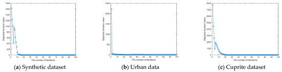
Figure 2.
Convergence analyses of AGBM-SV were experimentally performed on the Synthetic dataset, the Urban dataset and the Cuprite dataset.
3. Experiments and Result
In this section, we conduct simulation experiments on both synthetic and real HSI to demonstrate the unmixing performance and advantages of the proposed AGBM-SV. The proposed AGBM-SV algorithm is compared with several unmixing algorithms, including fully constrained least squares (FCLS) [39], ELMM, SUnSAL [40], SULoRA [41], ALMM, GBM-LRR [42], MUA-SV [23], LMM-SBD [43]. It should be noted that the GBM-LRR algorithm does not consider spectral variability, and the FCLS, SCLSU, ELMM, SUnSAL, SULoRA, ALMM, MUA-SV and LMM-SBD algorithms are all based on the LMM framework to handle spectral variability.
As the optimization problem of variable dictionary learning is non-convex, it is important to initialize the data in the AGBM-SV algorithm. We use the SCLSU algorithm to initialize the abundance matrix and use an orthogonal matrix to initialize the spectral variability dictionary based on its properties [26]. For the endmember matrix, we first estimate the number of endmembers in the dataset using the Hysime algorithm [30], and then extract endmembers using VCA [31]. To ensure fair comparison, the experiments are conducted on the same computer with an Intel(R) Core(TM) i5-8250U CPU @ 1.60 GHz and 16 GB memory.
3.1. Synthetic Dataset Experiments
3.1.1. Synthetic Data Description
The synthetic dataset contains 200 × 200 pixels with 224 spectral bands in the VIS and NIR. We randomly select five different mineral materials from the United States Geological Survey (USGS) [31] as reference endmembers and generate a 200 × 200 abundance map using Gaussian fields, satisfying the ANC and ASC constraints. To make the synthetic data more realistic and reflect the spectral variability in real-world hyperspectral data, we applied scaling factors and complex noise to the spectral signature of each pixel, ensuring spectral variability in the provided synthetic data. Figure 3 shows a false color image of the synthetic data and five extracted endmembers.
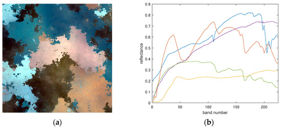
Figure 3.
(a) A false color representation of the synthetic dataset. (b) The five endmembers used for data simulation.
The implementation steps for the synthetic dataset are as follows: First, considering that each pixel in a real scene is unlikely to contain many endmembers, five endmembers are set to ensure sparsity of abundance, and the spectral features of the given reference endmembers are multiplied by spectral variability scaling factors in the range of (0.75, 1.25). Secondly, 25 dB white Gaussian noise is added to the scaled reference endmembers. Then, nonlinear coefficients are uniformly set in the range of (0, 1) to obtain a nonlinear abundance matrix, which is mixed for each pixel. Finally, 25 dB white Gaussian noise is added to the generated pixels. For more details on this dataset, refer to [20]. Through this process, a 200 × 200 × 224 simulated hyperspectral image is generated, and this simulated data of spectral variability can provide a more realistic experimental scenario. The spectral variations in this simulated data will provide an appropriate scenario to verify the proposed method.
3.1.2. Parameters Setting
Since the performance of the proposed AGBM-SV model is sensitive to the setting of the regularization parameters and the number of basis vectors (D) in the spectral variability dictionary , we tuned the above five parameters in the synthetic dataset to determine the optimal combination of parameters for solving the objective function. In order to accurately estimate abundances in AGBM-SV, the aRMSE is used as an important metric for parameter tuning. Throughout the entire experimental process, a grid search strategy is employed. Specifically, the optimal value for each parameter is evaluated while keeping the other parameter fixed until the lowest aRMSE value is achieved.
Figure 4 illustrates the test results for the above five parameters, showing that the performance of the AGBM-SV method is most sensitive to parameters D and . It also demonstrates the positive impact of selecting appropriate parameter values on unmixing performance. The optimal parameters D and were determined using an approximate convex curve. So the parameters of the proposed AGBM-SV method are set as α = 1 × 10⁻³, β = 3 × 10⁻⁶, γ = 1 × 10⁻², η = 3 × 10⁻⁴ and D = 125. To fairly assess the unmixing performance, the optimal parameters for all of the involved methods are set and recorded as follows. For the SUnSAL, the sparsity regularization is parameterized by (1 × 10⁻³). The regularization parameter for the ELMM is set as (4 × 10⁻¹, 5 × 10⁻³, 1 × 10⁻³). The parameters for ALMM are set as (2 × 10⁻³, 2 × 10⁻³, 5 × 10⁻³, 5 × 10⁻³, 100), and the SU-LoRA’s parameters are (1 × 10⁻¹, 1 × 10⁻², 8 × 10⁻³). For the GBM-LRR, the parameters are set as (1 × 10⁻³, 1 × 10⁻³). The regularization parameter for the MUA-SV is set as (4 × 10⁻¹, 5 × 10⁻³, 1 × 10⁻³, 1 × 10⁻²) and patchsize is set to 4. For the LMM-SBD method, the parameters are set to (6 × 10⁻¹, 5 × 10⁻²) and the patchsize is set to 5.
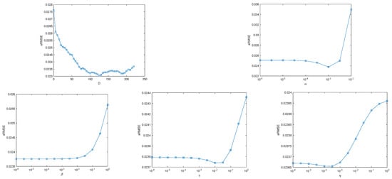
Figure 4.
Sensitivity analysis of 5 regularization parameters using the proposed AGBM-SV algorithm on synthetic dataset ( and the number of basis vectors (D) of ).
3.1.3. Evaluation Criteria
To evaluate the overall performance of the algorithm, we use the following four metrics to quantify the experimental results: signal reconstruction error (SRE), abundance overall root mean square error (aRMSE), reconstruction overall root mean square error (rRMSE), and average spectral angle mapper (aSAM).
(1) In simulation experiments, the SRE can be used to evaluate the performance of different hyperspectral unmixing algorithms on hyperspectral data with known ground truth abundance maps. The SRE measures the power between the signal and the error, and is defined as follows:
where and are the reference abundance matrix and the estimated abundance matrix obtained from the unmixing algorithm, respectively. The higher the SRE (dB) value, the better the algorithm’s unmixing performance.
(2) Similarly, we can employ aRMSE to measure the distance between the true abundance and the estimated abundance, which is defined as follows:
where and represent the corresponding true and estimated abundances for each pixel. Generally, the smaller the value of aRMSE, the smaller the difference between the true and estimated abundances. This indicates a better unmixing performance of the algorithm.
(3) For some real datasets, the true abundance map is generally unknown, so another evaluation metric can be defined from the perspective of data reconstruction to assess the performance of the algorithm. One of the evaluation metrics is rRMSE, defined by:
where and represent the actual spectral signals and the estimated spectral signals for each pixel, respectively.
(4) Similarly, aSAM can be used to evaluate the difference between the actual spectral signal and the reconstructed spectral signal, expressed as:
Generally, the smaller the rRMSE and aSAM values, the better the algorithm performance.
3.1.4. Results and Analysis
Table 1 shows the quantitative evaluation results for different algorithms. In addition to using the four evaluation metrics (aRMSE, rRMSE, aSAM, SRE) to assess the algorithms, a classification-based evaluation strategy is employed to approximate the overall accuracy (OA) of the abundance maps for each method. Initially, a spectral angle mapper (SAM) is used to generate rough classification results, where positive samples are labeled using cosine similarity and negative samples are masked with 0. For the spectral unmixing results of all methods, a classification map is obtained by assigning each pixel to the endmember with the highest abundance value. Finally, the OA for different methods is computed using the SAM classification results as the ground truth.

Table 1.
Quantitative performance comparison with the different algorithms on the synthetic dataset. The best algorithm is marked in bold.
From Table 1, it can be concluded that the classical linear unmixing model FCLSU shows the worst results in all of the evaluation metrics (aRMSE, rRMSE, OA, aSAM, SRE). SUnSAL methods can achieve relatively low aRMSE values and high SRE values compared with FCLSU. However, in terms of reconstruction error metrics, the rRMSE and aSAM values are relatively high, so the overall evaluation of the effectiveness of SUnSAL is not ideal. The SULoRA method shows relatively high values for aRMSE, rRMSE, and aSAM metrics, and a relatively low abundance reconstruction error (SRE) compared with SUnSAL. Compared with the above methods, ELMM and ALMM algorithms, which consider the spectral variability characteristics, have better results in all indicators, but they are still slightly inferior to the proposed AGBM-SV method. Similarly, the evaluation metrics for the MUA-SV and LMM-SBD methods, which consider spatial features, are inferior to those of the AGBM-SV method. The GBM-LRR method only considers the nonlinear effects in the data, but this leads to a large aRMSE metric value. Therefore, this indicates that spectral variability should be fully considered in nonlinear models. The proposed AGBM-SV method can simultaneously address the issues of nonlinearity and spectral variability, and its experimental results perform the best among all quantitative indicators (aRMSE, rRMSE, OA, aSAM, SRE). Moreover, from Figure 5a in the visualization of the aRMSE metric, it is also evident that the AGBM-SV method outperforms the other comparative methods. On the other hand, the required running time is relatively long due to the additional processing steps required by the AGBM-SV method and the influence of the adjusted parameters in the model.
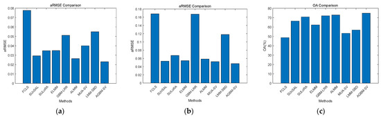
Figure 5.
Visualization of the aRMSE evaluation metric between different algorithms for the Synthetic dataset and Urban dataset, and the OA evaluation metric for the Cuprite dataset. (a) Synthetic; (b) Urban; (c) Cuprite.
As can be seen in Figure 6, the first image in the first row represents the false-color image of the synthetic dataset, while the remaining images in the row depict the classification results obtained by all methods based on the estimated abundance values. The second to sixth rows show the reference abundance maps and the corresponding estimated abundance maps by different algorithms, where each row represents a specific material, and each column represents a comparative method. We can clearly observe that the abundance map estimated by FCLSU has the largest deviation from the reference abundance map. This is because FCLSU needs to estimate the abundance within a simplex, which leads to large errors and also confirms that FCLSU has the worst quantitative evaluation results. GBM-LRR considers nonlinearity and sets low-rank constraints, but it treats spectral variability as nonlinearity, which results in poor estimation of abundance maps. The SUnSAL algorithm shows a noticeable improvement in unmixing performance. ELMM can model the scaling factors with reasonable prior information, but the estimated abundance maps contain obvious noise. ALMM improves the unmixing performance of the algorithm by considering both the scaling factors and other spectral variability factors. SULoRA achieves relatively distinct abundance maps by exploiting low-rank subspace effects and by setting sparse constraints, but the abundance of the last endmember appears too sparse. It is evident that the abundance maps estimated by LMM-SBD are influenced by different endmembers and deviate significantly from the ground truth abundance maps. As expected, the performance of the proposed AGBM-SV method is superior to all the compared methods, revealing that better abundance maps can be obtained when considering both nonlinearity and spectral variability.
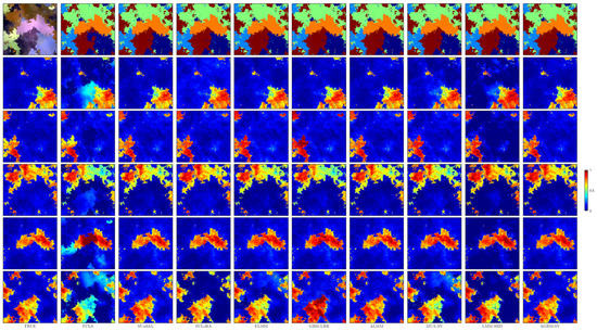
Figure 6.
Reference abundance maps and the estimated abundance maps obtained by using all the tested methods for the synthetic dataset. The first row represents the classification results obtained by different methods based on estimated abundance values.
3.2. Real Dataset Experiments
3.2.1. Urban Dataset
The first real dataset uses hyperspectral data, which was collected in an urban area of Copperas Cove, TX, USA, and has been widely used in research on hyperspectral unmixing. The version of data we used was captured by the Hyperspectral Digital Imagery Collection Experiment (HYDICE) sensor in 1995, which includes 307 × 307 pixels and 210 spectral bands with a spectral resolution of 10-nm, ranging from 400 to 2500 nm. As the dataset was also affected by some water absorption and noise during acquisition, we removed bands 1–4, 76, 87, 101–111, 136–153, and 198–210, resulting in the use of 162 bands in the experiments. Figure 7 shows a false color image of the study scene and the endmembers used in spectral unmixing.
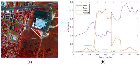
Figure 7.
(a) A false color representation of the urban dataset. (b) Four endmembers extracted by VCA in spectral unmixing.
Four main endmembers can be observed in the urban dataset: trees, grass, roof, and asphalt. Likewise, Hysime and VCA are adopted to determine the number of endmembers and build the endmember dictionary for all algorithms, respectively. Then, the endmembers can be identified by calculating the spectral angle of the estimated and reference endmembers. To fairly assess the unmixing performance, we utilize the optimal parameters as described in the literature. For the SUnSAL, the sparsity regularization is parameterized by (3 × 10⁻³). The regularization parameter for the ELMM is set as (4 × 10⁻¹, 1 × 10⁻³, 3 × 10⁻³). The parameters for ALMM are set as (5 × 10⁻², 5 × 10⁻², 1 × 10⁻², 1 × 10⁻², 80), and the SULoRA’s parameters are (1 × 10⁻¹, 1 × 10⁻², 5 × 10⁻³). For the GBM-LRR, parameters are (1 × 10⁻³, 5 × 10⁻³). For the MUA-SV, parameters are set as (5 × 10⁻¹, 3 × 10⁻¹, 1 × 10⁻⁴, 1 × 10⁻³) and patchsize is set to 4. For the LMM-SBD method parameters are set to (1 × 10⁻¹, 1 × 10⁻¹) and the patchsize is set to 8. To maximize the demonstration of the algorithm’s performance, a grid search strategy is also employed to determine the regularization parameters of the AGBM-SV model. Therefore, the optimal parameter settings for the AGBM-SV method are determined as α = 3 × 10⁻⁴, β = 3 × 10⁻², γ = 3 × 10⁻², η = 3 × 10⁻², and D = 40.
3.2.2. Result and Analysis of the Urban Dataset
As the urban dataset comes with a ground truth abundance map, the same five evaluation metrics (aRMSE, rRMSE, OA, aSAM, SRE) as for the synthetic data can be calculated for quantitative evaluation of the experimental results. Table 2 presents the quantitative evaluation results among all algorithms. From this, it can be concluded that the evaluation metrics of FCLSU are the worst among all the compared methods. In addition, compared with FCLSU without sparse constraint, SUnSAL shows relatively high SRE values, indicating that the mixed pixels in hyperspectral scenes are composed of a small number of spectral combinations of materials. SULoRA, ELMM and ALMM obtained similar results with low aRMSE and high SRE values for abundance estimation. Meanwhile, ELMM and ALMM showed relatively small reconstruction error values (rRMSE, aSAM). Although MUA-SV and LMM-SBD, which consider the spatial correlation of neighboring pixels, have lower time efficiency, their evaluation metrics are relatively poorer compared with the results of the AGBM-SV method. The proposed AGBM-SV method uses scaling factors and a spectral variability dictionary in nonlinear modeling to overcome spectral variability, resulting in better quantitative evaluation results than all comparison methods. Figure 5b visualizes the results of the aRMSE metric for different methods on this dataset, and it can be observed that the AGBM-SV method has smaller aRMSE values compared with all the comparative methods. Regarding the time efficiency of the algorithm, although AGBM-SV requires a longer time, it is still much faster than ELMM and ALMM in terms of runtime.
Table 2.
Quantitative evaluation of unmixing results for the urban dataset. The best results are marked in bold.
Figure 8 shows the reference abundance maps and the estimated abundance maps obtained by using all of the tested methods for endmembers: trees, grass, roof, and asphalt. Similarly, the first row shows the classification results of different methods. Visually, the classical FCLS mixing method cannot effectively detect all endmembers and obtain accurate abundances. SUnSAL is able to effectively detect most of the materials in the scene, but some trees are incorrectly identified as grass components. As shown in the fifth row of Figure 8. SULoRA obtains a purer identification for the materials of asphalt, while there is still room for improvement in the abundance estimation of grass, trees, and roof. Although ELMM considers scaling factors, it is difficult to interpret all endmember regions. Therefore, it incorrectly estimates the abundance maps of some asphalt and roof materials, as shown in the sixth row of Figure 8. ALMM can obtain good identification results for asphalt and roof materials, but there are errors in the identification of grassland and trees. The reason for this is that the nonlinear effects between grassland and trees have not been fully considered. GBM-LRR had significant errors for all four materials, as it only considers the nonlinearity caused by the second order scattering among multiple materials, and the spectral variability that occurs in real scenes is excessively absorbed by the nonlinear term. Additionally, it is visually clear that MUA-SV has a small error in identifying grassland, while the LMM-SBD method shows a significant difference between the estimated abundance of all endmembers and the true abundance map. As shown in the last column of Figure 8, the abundance maps estimated by our proposed AGBM-SV method are consistent with the ground truth, and the contrast among different endmembers is clearer. Therefore, the proposed method can effectively handle spectral variability in nonlinear models.
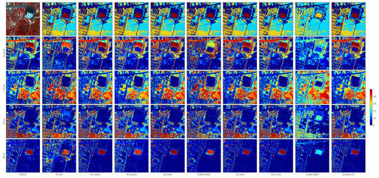
Figure 8.
Reference abundance maps and the estimated abundance maps obtained by using all of the tested methods for the Urban dataset.
3.2.3. Cuprite Dataset
The second real dataset is a hyperspectral image of the Cuprite mining area in western Nevada, USA, collected by the AVIRIS sensor. This mining area is composed of multiple minerals. This instrument has 224 spectral bands, with a wavelength range of 400–2500 nm and a spectral resolution of 10 nm. Evaluation was undertaken of the performance of the AGBM-SV method and the comparative methods on a sub-image of size 250 × 191 pixels. The reflectance image of Cuprite is corrected by removing the bands that are severely affected by water absorption, atmospheric effects, and noise. Only 188 bands are used in the experimental data. Figure 9 shows a false color image and the endmembers extracted by VCA of the used scene. It needs to be noted that the Cuprite dataset exhibits spectral variability and nonlinearity. For example, there is intra-class variability in the alunite material, which can result in multiple spectral reflections for the same endmember. Additionally, the scattered light from a given material is reflected by other materials before reaching the sensor, indicating the presence of nonlinear effects in the data.
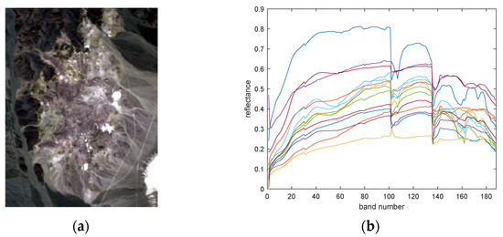
Figure 9.
(a) A false color image display of the cuprite dataset. (b) The fourteen endmembers extracted by VCA in spectral unmixing.
Likewise, the main fourteen materials in Cuprite are identified using Hysime, and endmembers are extracted using VCA. We visually compare the estimated abundance maps and endmember features with those recovered in [44] to confirm the materials. To fairly assess the unmixing performance, the optimal parameters for all the involved methods are set and recorded as follows. The sparsity regularization of the SUnSAL is parameterized by (5 × 10⁻³). The regularization parameter for the ELMM is set as (6 × 10⁻¹, 5 × 10⁻³, 1 × 10⁻²). The parameters for ALMM are set as (1 × 10⁻², 5 × 10⁻², 5 × 10⁻², 1 × 10⁻², 90), and the SULoRA’s parameters are (1 × 10⁻³, 1 × 10⁻², 3 × 10⁻³). For the GBM-LRR, the sparsity and low-rank regularizations are parameterized by (3 × 10⁻³, 1 × 10⁻²). The regularization parameter for the MUA-SV is set as (5 × 10⁻¹, 1 × 10⁻², 5 × 10⁻², 1 × 10⁻²) and patchsize is set to 6. For the LMM-SBD method parameters are set to (1 × 10⁻¹, 2 × 10⁻¹) and the patchsize is set to 28. The parameters of the proposed AGBM-SV method are set as α = 3 × 10⁻⁴, β = 3 × 10⁻³, γ = 1 × 10⁻⁶, η = 1 × 10⁻¹ and D = 155.
3.2.4. Result and Analysis of Cuprite
Due to the high mixing effect between minerals and the lack of true abundance maps, some endmembers are quantitatively and visually evaluated. To highlight the differences in abundance maps, we used the abundance maps obtained by extracting endmembers using VCA as the reference abundances [31]. For quantitative evaluation, the rRMSE and aSAM are calculated from the perspective of signal reconstruction. In order to effectively utilize OA for quantitative evaluation of the performance of different algorithms, we only considered four main minerals: Alunite, Muscovite, Kaolinite, and Buddingtonite. Figure 10 shows the abundance maps of some endmembers for all of the compared algorithms, as well as the classification results obtained based on the estimated abundance values. The reconstruction errors, OA and running times of all the algorithms are shown in Table 3. In terms of running time, FCLSU, SUnSAL, SULoRA and LMM-SBD algorithms are fast due to their simple implementation. Although the running time of the AGBM-SV method is influenced by the preprocessing steps and regularization parameters in the model, it is still much faster than GBM-LRR and ELMM while achieving the highest unmixing accuracy. Furthermore, Figure 5c visually presents the results of OA for different methods on the dataset, indicating that the AGBM-SV method has a higher OA value compared with all of the comparative methods.

Figure 10.
The abundance maps comparison between the proposed method and the state-of-the-art methods. The first row represents the classification results obtained by different methods based on estimated abundance values.
Table 3.
Quantitative evaluation of unmixing results in the Cuprite dataset. The best results are marked in bold.
Based on the other quantitative and visual results, we performed the following analysis of algorithm performance. The FCLSU abundance map strictly follows ANC and ASC, and does not consider spectral variability, resulting in missing parts of the Alunite material. SUnSAL improved the visual performance by relaxing the ASC, but the evaluated rRMSE, aSAM and OA metrics are relatively high. Although SULoRA uses low-rank subspace to handle spectral variability, the estimated abundance maps of this method have large errors. As shown in the fourth row of Figure 10, SULoRA underestimated the abundance of Buddingtonite and could not correctly identify Kaolinite material. ELMM and GBM-LRR estimated abundances are mostly consistent and the reconstruction error rRMSE evaluation metric is relatively small compared with SULoRA. The abundance maps of Muscovite and Kaolinite estimated by ALMM are affected by other mineral materials in the background region. This is caused by the inability of ALMM to handle the non-linear effects that exist between closely spaced minerals. Moreover, it is evident that LMM-SBD fails to accurately estimate the Kaolinite material, and that it is significantly influenced by the background area when estimating Alunite and Muscovite materials. The proposed AGBM-SV method achieves relatively low values in the quantitative measures of reconstruction error (OA, rRMSE, aSAM) compared with the comparison methods, and all estimated endmember abundance maps are more distinct and show greater contrast. These results reveal the potential of the proposed AGBM-SV method in dealing with spectral variability in nonlinear models.
4. Conclusions
In this paper, we proposed an augmented GBM nonlinear model to address the spectral variability in hyperspectral unmixing. The AGBM-SV method can ensure the consideration of spectral variability in nonlinear unmixing. The main advantage of this model is that it solves multiple scattering effects in real-world scenarios through GBM and handles spectral variability by introducing scaling factors and spectral variability dictionaries. Based on the characteristics of real-world material distribution, the sparsity and orthogonality of the abundance matrix and spectral variability dictionary are constrained to guide the nonlinear unmixing. Additionally, reasonable initialization of the abundance and endmember matrices, and optimization of the objective function using multi-block ADMM, enhance the effectiveness and convergence of the AGBM-SV method.
In the experimental results on synthetic and real datasets, we found that the model that considers spectral variability estimated abundances more accurately than the model that does not. Moreover, the unmixing method that considers spectral variability during nonlinear unmixing was found to be superior to the method that only considers spectral variability. Therefore, the proposed AGBM-SV method can handle spectral variability well and obtain accurate abundance estimates for endmembers in nonlinear scenarios. Overall, this method is more effective and is superior to classical nonlinear or variability-based unmixing methods.
Our future work will focus on improving the execution efficiency of AGBM-SV, enabling it to achieve not only higher accuracy in abundance estimation but also faster processing speed. We also plan to explore automatic selection methods for regularization parameters to be applied in the AGBM-SV model. In terms of extending the applicability of this method, one potential direction is to incorporate prior knowledge to guide the unmixing process. This can involve considering the spatial correlation between neighboring pixels and utilizing additional data sources, such as Lidar data, to accurately estimate scaling factors and corresponding abundances. Such an extension will enhance the adaptability of this method to real-world scenarios and improve its performance in complex environments.
Author Contributions
Conceptualization, L.M.; methodology, L.M.; validation, X.Y. and Y.P.; formal analysis, L.M.; investigation, X.Y. and Y.P.; writing—original draft preparation, L.M.; writing—review and editing, D.L. and J.A.B.; visualization, L.M.; supervision, D.L. and J.A.B.; project administration, D.L.; funding acquisition, L.W. All authors have read and agreed to the published version of the manuscript.
Funding
This research was supported by Leading Talents Project of the State Ethnic Affairs Commission and National Natural Science Foundation of China (No. 62071084).
Data Availability Statement
Not applicable.
Acknowledgments
The authors sincerely thank the academic editors and reviewers for their useful comments and constructive suggestions.
Conflicts of Interest
The authors declare no conflict of interest.
Appendix A
The objective function in Equation (12) does not satisfy the condition of simultaneous convexity for all variables, but it is convex for each individual variable when other variables are fixed. Therefore, we decompose the objective function into individual subproblems and solve them separately. The specific process for decomposing and solving each subproblem in Equation (12) is as follows.
For the optimization of : The problem is transformed and solved in the following form:
For the optimization of : The objective function for the optimization of can be written as follows and solved:
For the optimization of : The objective function for the optimization of can be written as follows and solved:
where to satisfy the ASC constraint required by the objective function while removing the scaling factor, we rewrite in the following form:
where ./ represents matrix element-wise division.
For the optimization of : The objective function for the optimization of can be written as follows and solved:
For the optimization of : The objective function for the optimization of can be written as follows and solved:
For the optimization of : We can adopt the method proposed in [32], where we take as a fixed matrix throughout the current iteration process and obtain it from the previous iteration’s . Therefore, the optimization process of can be written as follows and solved:
For the optimization of : We use the well-known soft thresholding method [45]:
For the optimization of : The objective function for the optimization of can be written as follows and solved:
For the optimization of : The objective function for the optimization of can be written as follows and solved:
For the optimization of : The objective function for the optimization of can be written as follows and solved:
For the optimization of : The objective function for the optimization of can be written as follows and solved:
The following are updates to the Lagrangian multipliers in each iteration process:
References
- Bioucas-Dias, J.M.; Plaza, A.; Camps-Valls, G.; Scheunders, P.; Nasrabadi, N.; Chanussot, J. Hyperspectral remote sensing data analysis and future challenges. IEEE Geosci. Remote Sens. Mag. 2013, 1, 6–36. [Google Scholar] [CrossRef]
- Li, S.; Song, W.; Fang, L.; Chen, Y.; Ghamisi, P.; Benediktsson, J.A. Deep learning for hyperspectral image classification: An overview. IEEE Trans. Geosci. Remote Sens. 2019, 57, 6690–6709. [Google Scholar] [CrossRef]
- Pan, Y.; Liu, D.; Wang, L.; Benediktsson, J.A.; Xing, S. A Pan-sharpening method with beta-divergence non-negative matrix factorization in non-subsampled shear transform domain. Remote Sens. 2022, 14, 2921. [Google Scholar] [CrossRef]
- Yokoya, N.; Iwasaki, A. Object detection based on sparse representation and hough voting for optical remote sensing imagery. IEEE J. Sel. Top. Appl. Earth Obs. Remote Sens. 2015, 8, 2053–2062. [Google Scholar] [CrossRef]
- Borsoi, R.A.; Imbiriba, T.; Bermudez, J.C.M.; Richard, C.; Chanussot, J.; Drumetz, L.; Tourneret, J.-Y.; Zare, A.; Jutten, C. Spectral variability in hyperspectral data unmixing: A comprehensive review. IEEE Geosci. Remote Sens. Mag. 2021, 9, 223–270. [Google Scholar] [CrossRef]
- Keshava, N.; John, F.M. Spectral unmixing. IEEE Signal Process. Mag. 2002, 19, 44–57. [Google Scholar] [CrossRef]
- Heylen, R.; Mario, P.; Paul, G. A review of nonlinear hyperspectral unmixing methods. IEEE J. Sel. Top. Appl. Earth Obs. Remote Sens. 2014, 7, 1844–1868. [Google Scholar] [CrossRef]
- Dobigeon, N.; Tourneret, J.-Y.; Richard, C.; Bermudez, J.C.M.; McLaughlin, S.; Hero, A.O. Nonlinear unmixing of hyperspectral images: Models and algorithms. IEEE Signal Process. Mag. 2013, 31, 82–94. [Google Scholar] [CrossRef]
- Zare, A.; Ho, K. Endmember variability in hyperspectral analysis: Addressing spectral variability during spectral unmixing. IEEE Signal Process. Mag. 2013, 31, 95–104. [Google Scholar] [CrossRef]
- Drumetz, L.; Meyer, T.R.; Chanussot, J.; Bertozzi, A.L.; Jutten, C. Hyperspectral image unmixing with endmember bundles and group sparsity inducing mixed norms. IEEE Trans. Image Process. 2019, 28, 3435–3450. [Google Scholar] [CrossRef]
- Zhang, G.; Mei, S.; Xie, B.; Ma, M.; Zhang, Y.; Feng, Y.; Du, Q. Spectral variability augmented sparse unmixing of hyperspectral images. IEEE Trans. Geosci. Remote Sens. 2022, 60, 1–13. [Google Scholar] [CrossRef]
- Somers, B.; Asner, G.P.; Tits, L.; Coppin, P. Endmember variability in spectral mixture analysis: A review. Remote Sens. Environ. 2011, 115, 1603–1616. [Google Scholar] [CrossRef]
- Ammanouil, R.; Ferrari, A.; Richard, C.; Mathieu, S. Nonlinear unmixing of hyperspectral data with vector-valued kernel functions. IEEE Trans. Image Process. 2016, 26, 340–354. [Google Scholar] [CrossRef] [PubMed]
- Heylen, R.; Scheunders, P. A Multilinear mixing model for nonlinear spectral unmixing. IEEE Trans. Geosci. Remote Sens. 2015, 54, 240–251. [Google Scholar] [CrossRef]
- Marinoni, A.; Plaza, J.; Plaza, A.; Gamba, P. Estimating nonlinearities in p-linear hyperspectral mixtures. IEEE Trans. Geosci. Remote Sens. 2018, 56, 6586–6595. [Google Scholar] [CrossRef]
- Tang, M.; Zhang, B.; Marinoni, A.; Gao, L.; Gamba, P. Multiharmonic postnonlinear mixing model for hyperspectral nonlinear unmixing. IEEE Geosci. Remote Sens. Lett. 2018, 15, 1765–1769. [Google Scholar] [CrossRef]
- Halimi, A.; Altmann, Y.; Dobigeon, N.; Tourneret, J.-Y. Unmixing hyperspectral images using the generalized bilinear model. In Proceedings of the 2011 IEEE International Geoscience and Remote Sensing Symposium, Vancouver, BC, Canada, 24–29 July 2011. [Google Scholar]
- Yokoya, N.; Chanussot, J.; Iwasaki, A. Nonlinear unmixing of hyperspectral data using semi-nonnegative matrix factorization. IEEE Trans. Geosci. Remote Sens. 2013, 52, 1430–1437. [Google Scholar] [CrossRef]
- Yang, B.; Wang, B.; Wu, Z. Nonlinear hyperspectral unmixing based on geometric characteristics of bilinear mixture models. IEEE Trans. Geosci. Remote Sens. 2017, 56, 694–714. [Google Scholar] [CrossRef]
- Fan, W.; Hu, B.; Miller, J.; Li, M. Comparative study between a new nonlinear model and common linear model for analysing laboratory simulated-forest hyperspectral data. Int. J. Remote Sens. 2009, 30, 2951–2962. [Google Scholar] [CrossRef]
- Drumetz, L.; Veganzones, M.-A.; Henrot, S.; Phlypo, R.; Chanussot, J.; Jutten, C. Blind hyperspectral unmixing using an extended linear mixing model to address spectral variability. IEEE Trans. Image Process. 2016, 25, 3890–3905. [Google Scholar] [CrossRef]
- Thouvenin, P.-A.; Dobigeon, N.; Tourneret, J.-Y. Hyperspectral unmixing with spectral variability using a perturbed linear mixing model. IEEE Trans. Signal Process. 2015, 64, 525–538. [Google Scholar]
- Borsoi, R.A.; Tales, I.; Jose, C.M.B. A data dependent multiscale model for hyperspectral unmixing with spectral variability. IEEE Trans. Image Process. 2020, 29, 3638–3651. [Google Scholar] [CrossRef] [PubMed]
- Revel, C.; Deville, Y.; Achard, V.; Briottet, X. A linear-quadratic unsupervised hyperspectral unmixing method dealing with intra-class variability. In Proceedings of the 2016 8th Workshop on Hyperspectral Image and Signal Processing: Evolution in Remote Sensing (WHISPERS), Los Angeles, CA, USA, 21–24 August 2016. [Google Scholar]
- Li, C.; Liu, Y.; Cheng, J.; Song, R.; Peng, H.; Chen, Q.; Chen, X. Hyperspectral unmixing with bandwise generalized bilinear model. Remote Sens. 2018, 10, 1600. [Google Scholar] [CrossRef]
- Hong, D.; Yokoya, N.; Chanussot, J.; Zhu, X.X. An augmented linear mixing model to address spectral variability for hyperspectral unmixing. IEEE Trans. Image Process. 2019, 28, 1923–1938. [Google Scholar] [CrossRef]
- Drumetz, L.; Chanussot, J.; Jutten, C.; Ma, W.-K.; Iwasaki, A. Spectral variability aware blind hyperspectral image unmixing based on convex geometry. IEEE Trans. Image Process. 2020, 29, 4568–4582. [Google Scholar] [CrossRef] [PubMed]
- Veganzones, M.A.; Drumetz, L.; Tochon, G.; Mura, M.D.; Plaza, A.; Bioucas-Dias, J.-M.; Chanussot, J. A new extended linear mixing model to address spectral variability. In Proceedings of the 2014 6th Workshop on Hyperspectral Image and Signal Processing: Evolution in Remote Sensing (WHISPERS), Lausanne, Switzerland, 24–27 June 2014. [Google Scholar]
- Halimi, A.; Honeine, P.; Bioucas-Dias, J.M. Hyperspectral unmixing in presence of endmember variability, nonlinearity, or mismodeling effects. IEEE Trans. Image Process. 2016, 25, 4565–4579. [Google Scholar] [CrossRef]
- Bioucas-Dias, J.M.; José, M.P.N. Hyperspectral subspace identification. IEEE Trans. Geosci. Remote Sens. 2008, 46, 2435–2445. [Google Scholar] [CrossRef]
- Nascimento, J.M.P.; José, M.B.D. Vertex component analysis: A fast algorithm to unmix hyperspectral data. IEEE Trans. Geosci. Remote Sens. 2005, 43, 898–910. [Google Scholar] [CrossRef]
- Barchiesi, D.; Plumbley, M.D. Learning incoherent dictionaries for sparse approximation using iterative projections and rotations. IEEE Trans. Signal Process. 2013, 61, 2055–2065. [Google Scholar]
- Bioucas-Dias, J.M.; Figueiredo, M.A.T. Alternating direction algorithms for constrained sparse regression: Application to hyperspectral unmixing. In Proceedings of the 2010 2nd Workshop on Hyperspectral Image and Signal Processing: Evolution in Remote Sensing, Reykjavik, Iceland, 14–16 June 2010. [Google Scholar]
- Boyd, S.; Parikh, N.; Chu, E.; Peleato, B.; Eckstein, J. Distributed optimization and statistical learning via the alternating direction method of multipliers. Found. Trends® Mach. Learn. 2011, 3, 1–122. [Google Scholar]
- Liu, Q.; Shen, X.; Gu, Y. Linearized ADMM for nonconvex nonsmooth optimization with convergence analysis. IEEE Access 2019, 7, 76131–76144. [Google Scholar] [CrossRef]
- Wang, F.; Cao, W.; Xu, Z. Convergence of multi-block Bregman ADMM for nonconvex composite problems. Sci. China Inf. Sci. 2018, 61, 122101. [Google Scholar] [CrossRef]
- Zhou, P.; Zhang, C.; Lin, Z. Bilevel model-based discriminative dictionary learning for recognition. IEEE Trans. Image Process. 2016, 26, 1173–1187. [Google Scholar] [CrossRef] [PubMed]
- Xu, Y.; Yin, W.; Wen, Z.; Zhang, Y. An alternating direction algorithm for matrix completion with nonnegative factors. Front. Math. China 2012, 7, 365–384. [Google Scholar] [CrossRef]
- Heinz, D.C. Fully constrained least squares linear spectral mixture analysis method for material quantification in hyperspectral imagery. IEEE Trans. Geosci. Remote Sens. 2001, 39, 529–545. [Google Scholar] [CrossRef]
- Iordache, M.-D.; José, M. Bioucas-Dias, and Antonio Plaza. Sparse unmixing of hyperspectral data. IEEE Trans. Geosci. Remote Sens. 2011, 49, 2014–2039. [Google Scholar] [CrossRef]
- Hong, D.; Zhu, X.X. SULoRA: Subspace unmixing with low-rank attribute embedding for hyperspectral data analysis. IEEE J. Sel. Top. Signal Process. 2018, 12, 1351–1363. [Google Scholar] [CrossRef]
- Mei, X.; Ma, Y.; Li, C.; Fan, F.; Huang, J.; Ma, J. Robust GBM hyperspectral image unmixing with superpixel segmentation based low rank and sparse representation. Neurocomputing 2018, 275, 2783–2797. [Google Scholar] [CrossRef]
- Azar, S.G.; Meshgini, S.; Beheshti, S.; Rezaii, T.Y. Linear mixing model with scaled bundle dictionary for hyperspectral unmixing with spectral variability. Signal Process. 2021, 188, 108214. [Google Scholar] [CrossRef]
- Wang, Y.; Pan, C.; Xiang, S.; Zhu, F. Robust hyperspectral unmixing with correntropy-based metric. IEEE Trans. Image Process. 2015, 24, 4027–4040. [Google Scholar] [CrossRef]
- Cai, J.; Candès, E.J.; Shen, Z. A singular value thresholding algorithm for matrix completion. SIAM J. Optim. 2010, 20, 1956–1982. [Google Scholar] [CrossRef]
Disclaimer/Publisher’s Note: The statements, opinions and data contained in all publications are solely those of the individual author(s) and contributor(s) and not of MDPI and/or the editor(s). MDPI and/or the editor(s) disclaim responsibility for any injury to people or property resulting from any ideas, methods, instructions or products referred to in the content. |
© 2023 by the authors. Licensee MDPI, Basel, Switzerland. This article is an open access article distributed under the terms and conditions of the Creative Commons Attribution (CC BY) license (https://creativecommons.org/licenses/by/4.0/).