
A New Approach Combining a Multilayer Radiative Transfer Model with an Individual-Based Forest Model: Application to Boreal Forests in Finland


Abstract
1. Introduction
2. Materials and Methods
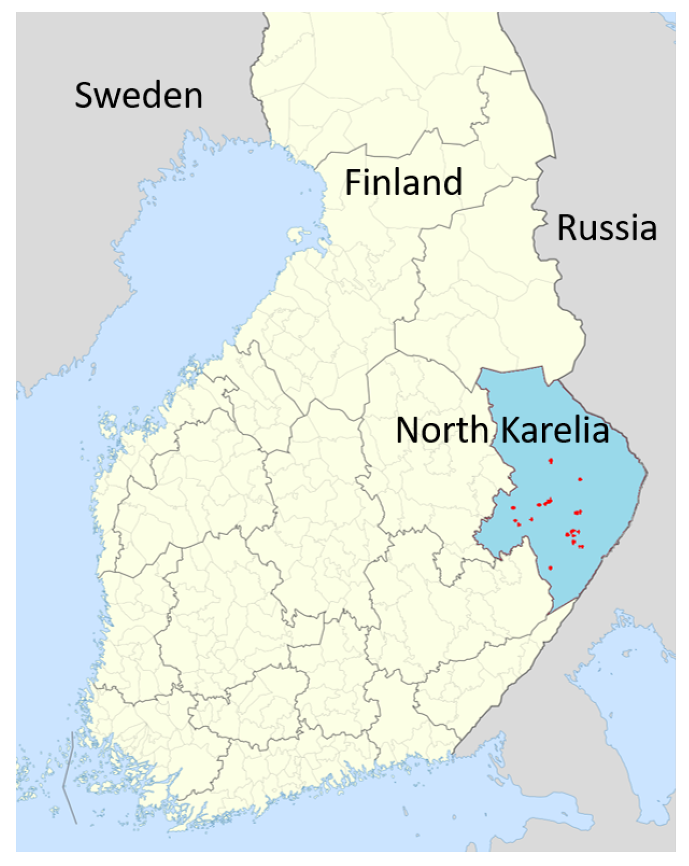
2.1. Study Site
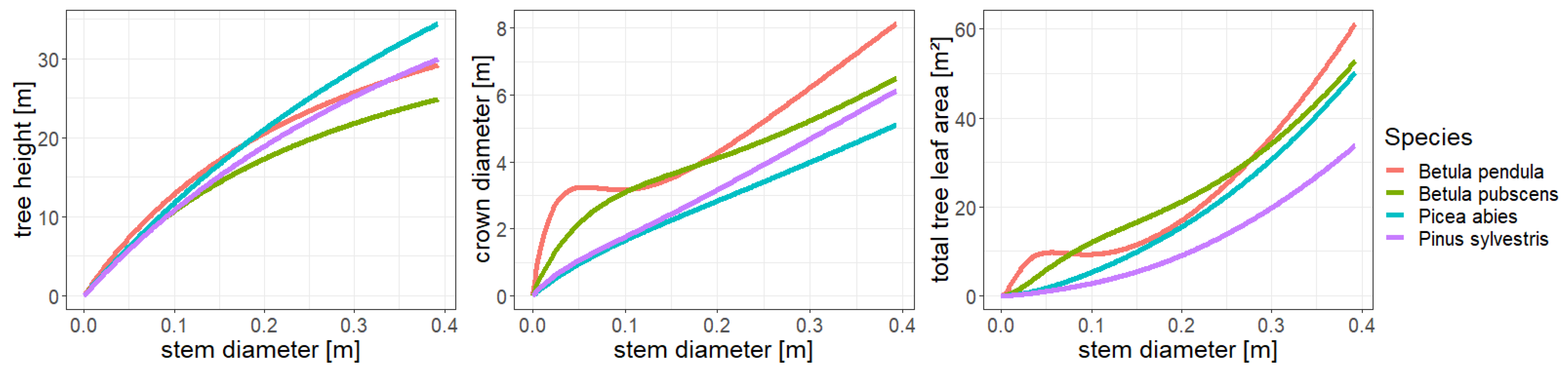
2.2. The Individual-Based Forest Model FORMIND
2.3. Coupling mScope with FORMIND
- Leaf structure (number of internal leaf layers [layer]);
- The amount of pigments in the leaf (chlorophyll a and b [g cm], carotenoids [g cm], anthocyanins [g cm], senescent pigments [fraction]);
- Dry matter [g cm] and leaf water content [g cm];
- Traits describing vegetation structure as the mean and bi-modality of the leaf inclination distribution function, LAI [m m], canopy height [m].
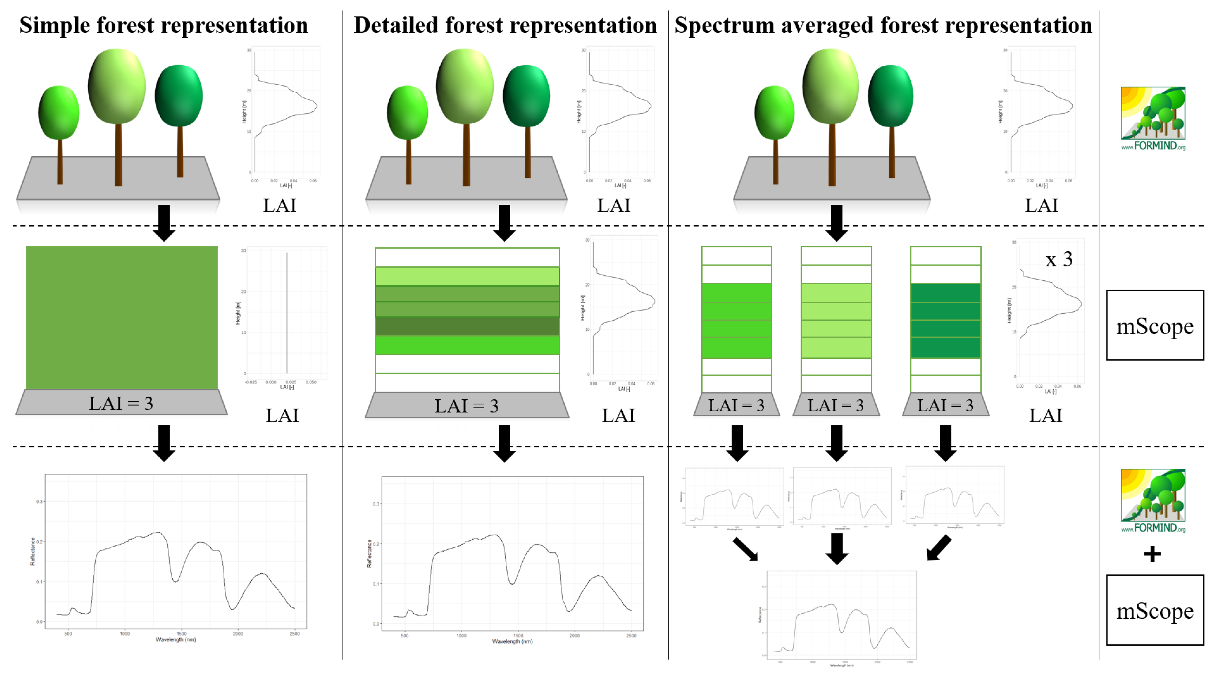
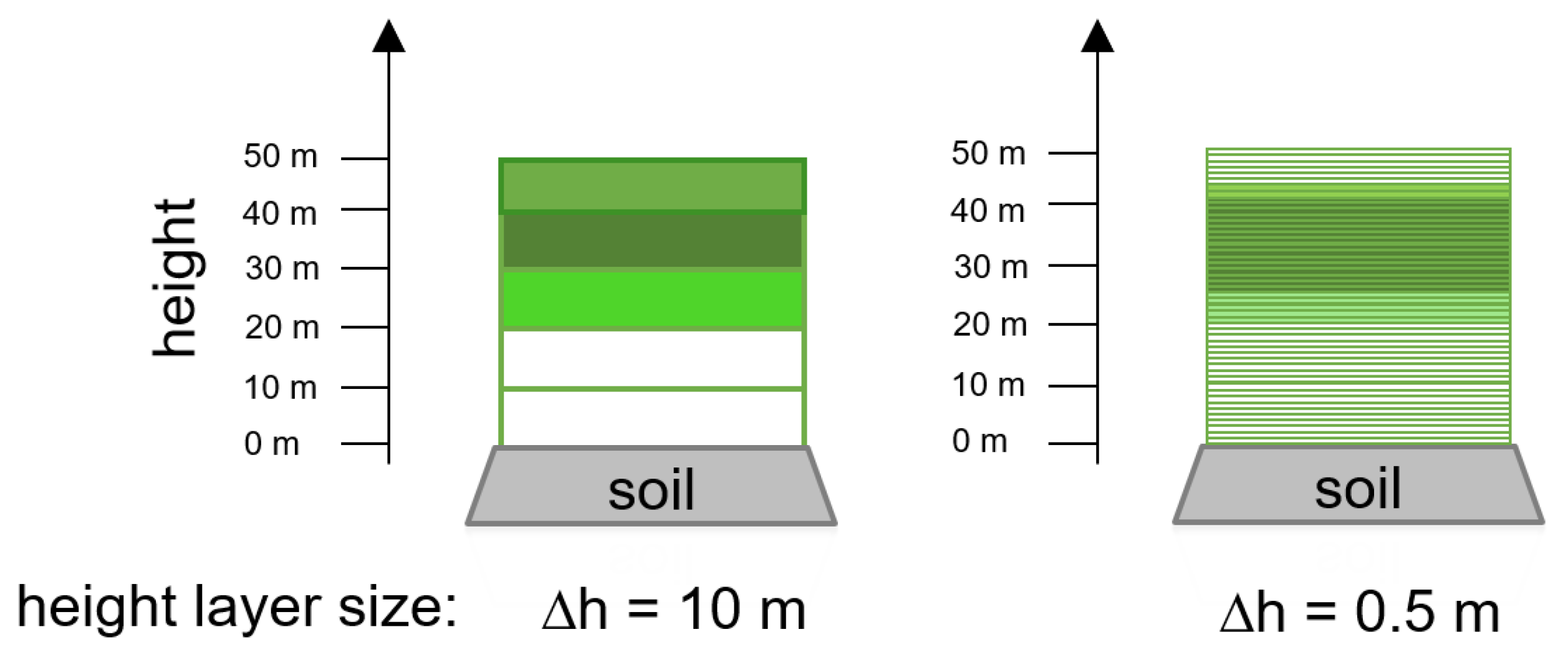
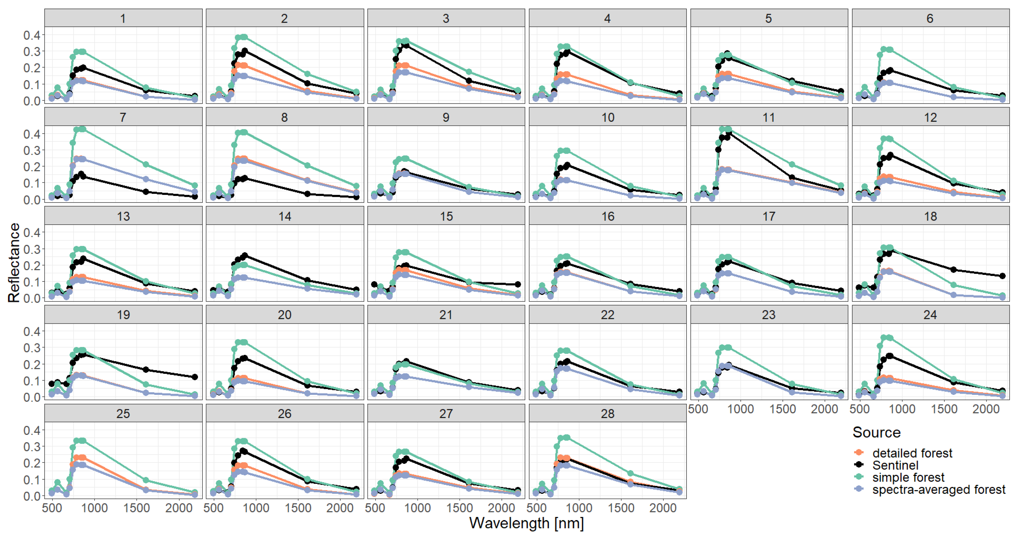
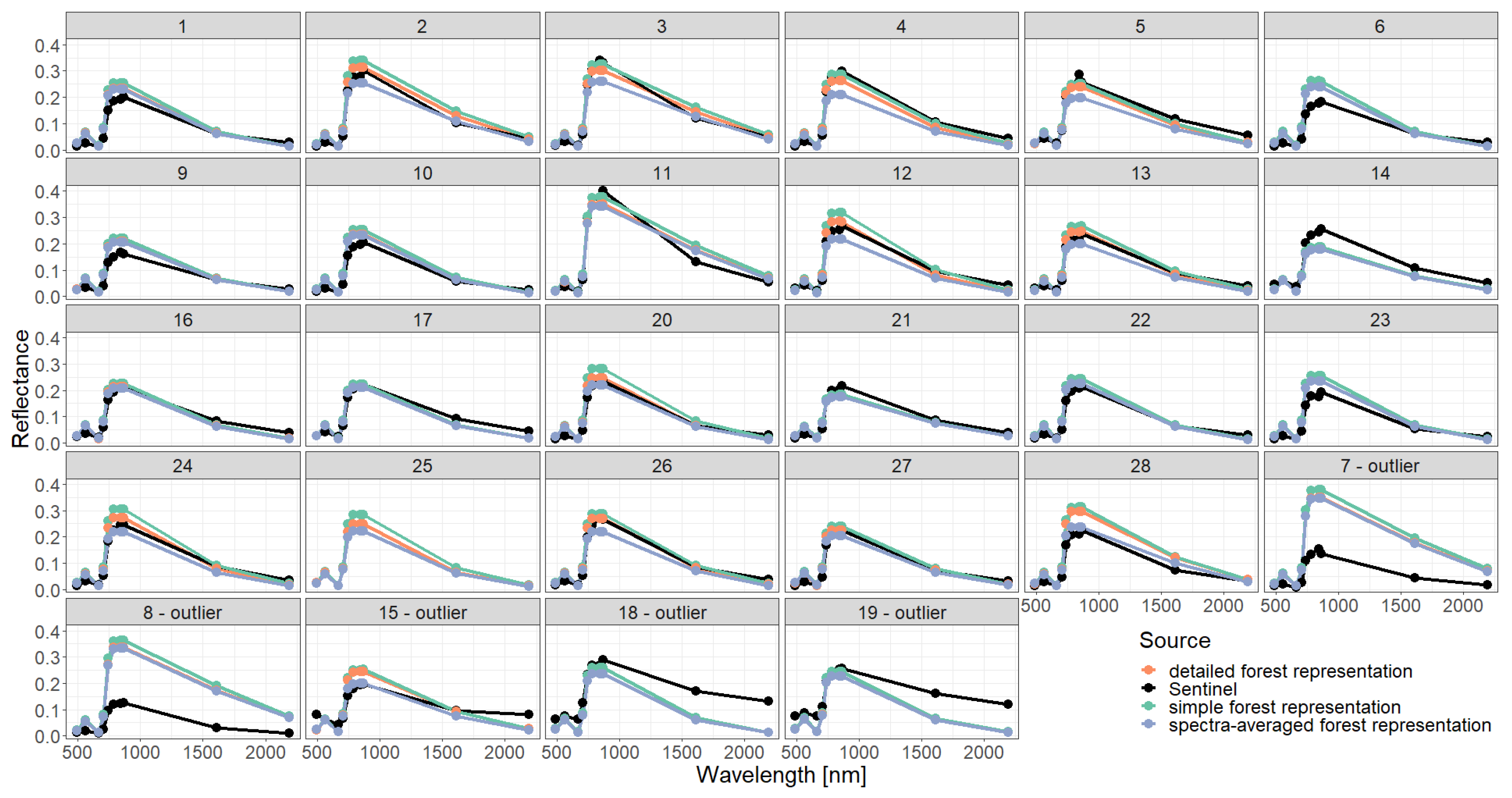
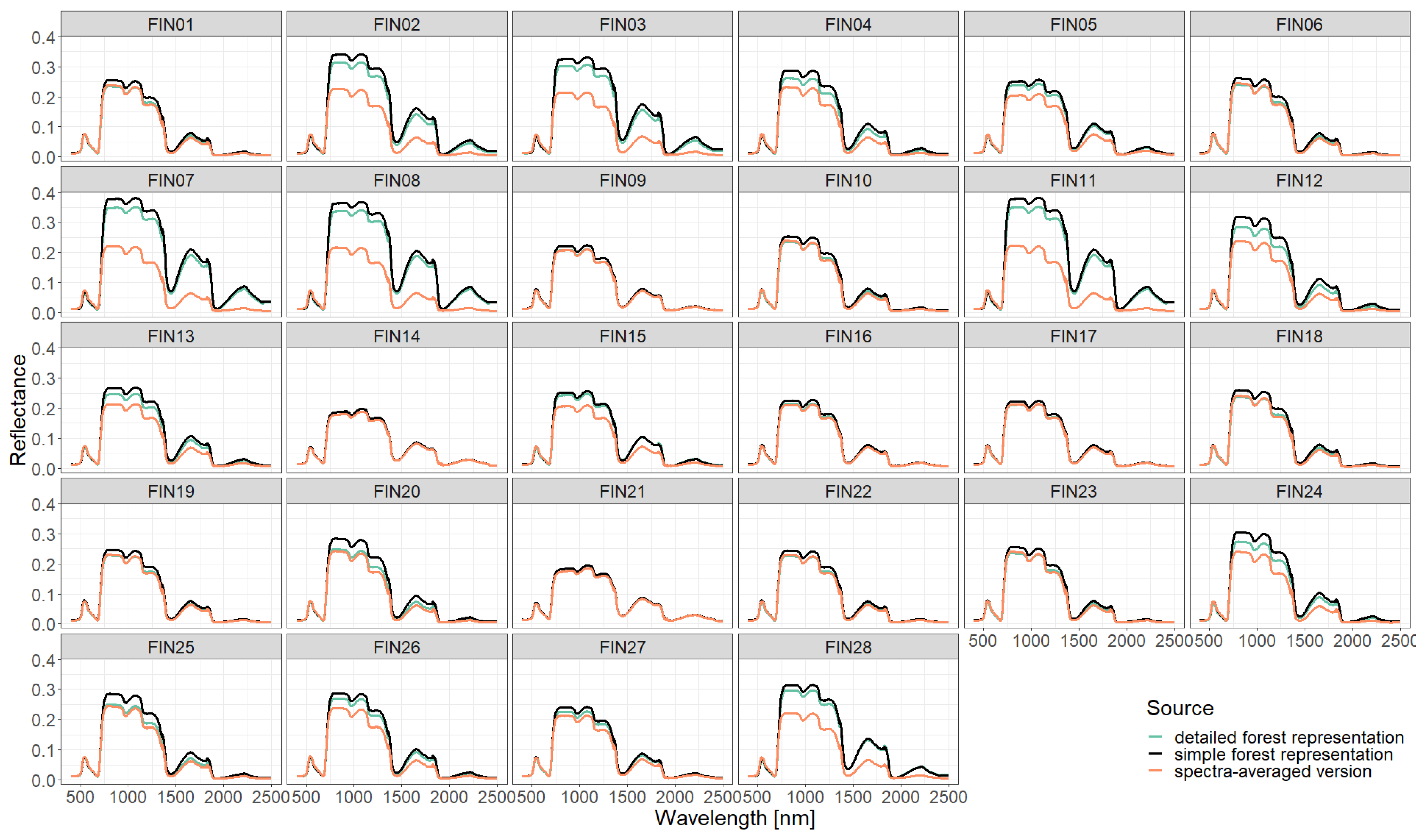
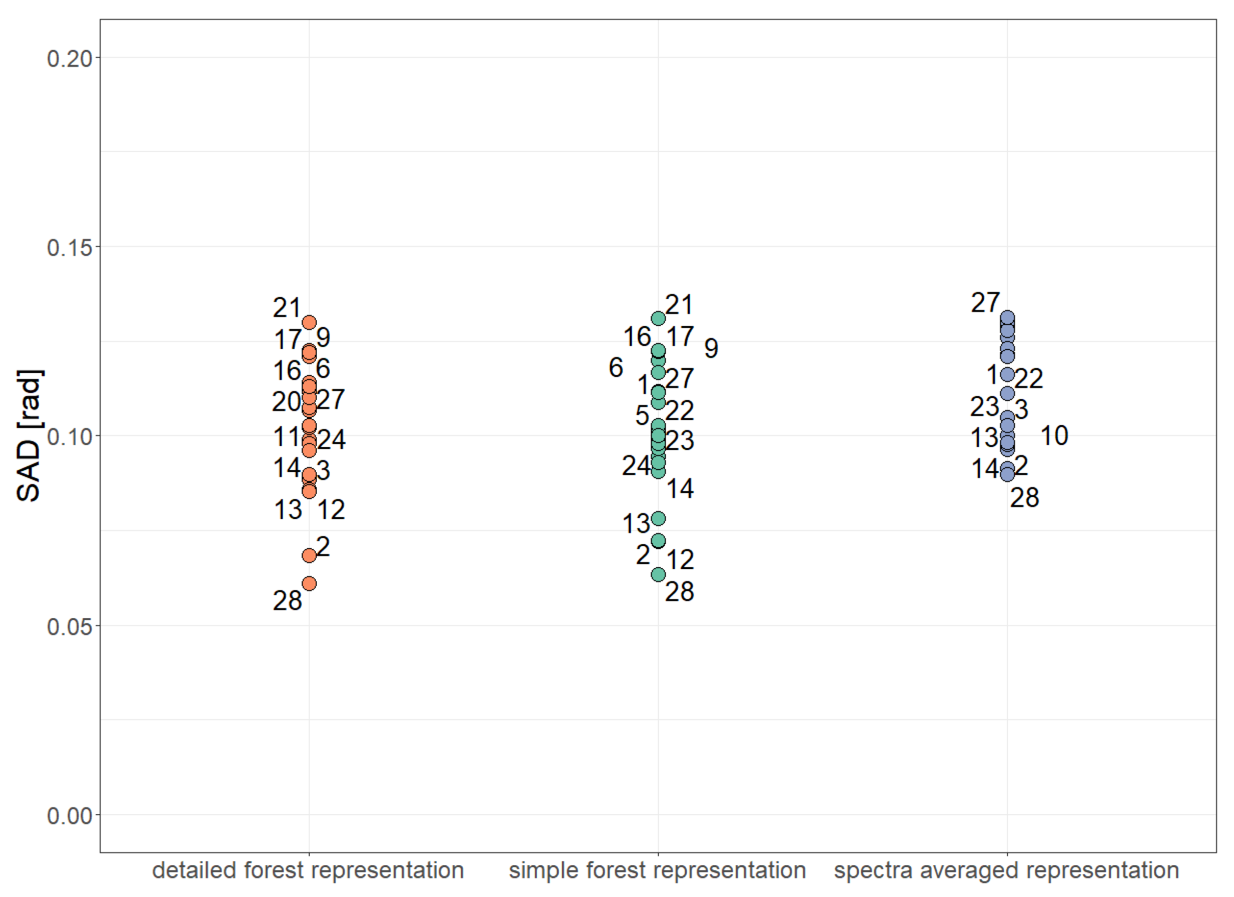
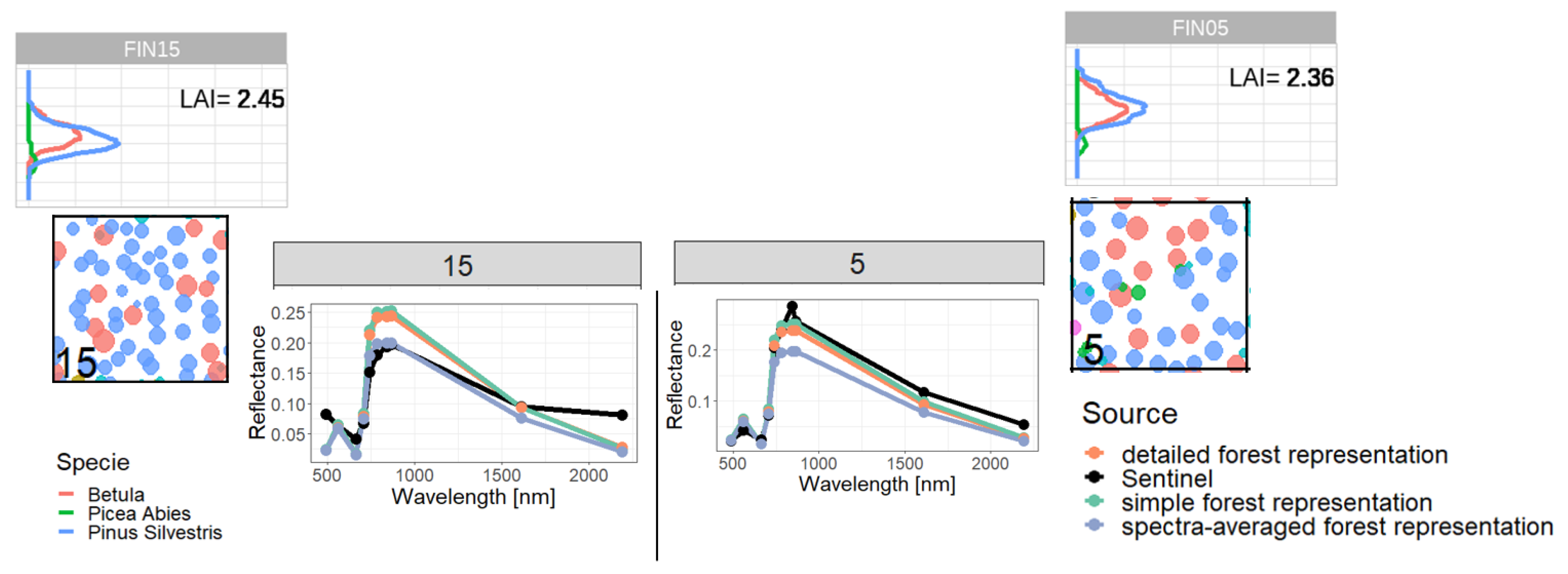
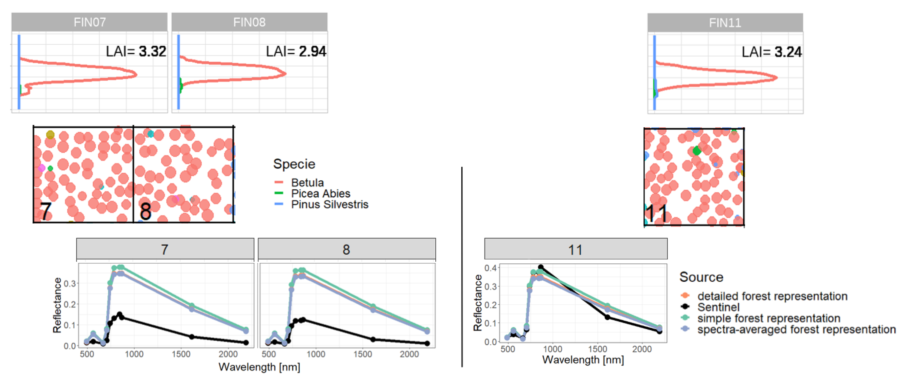
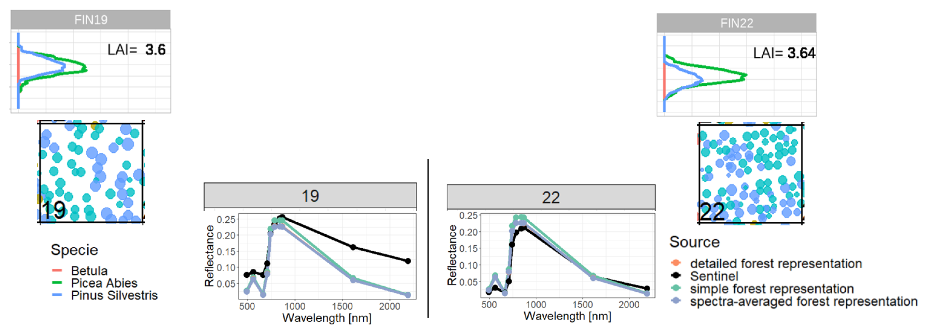
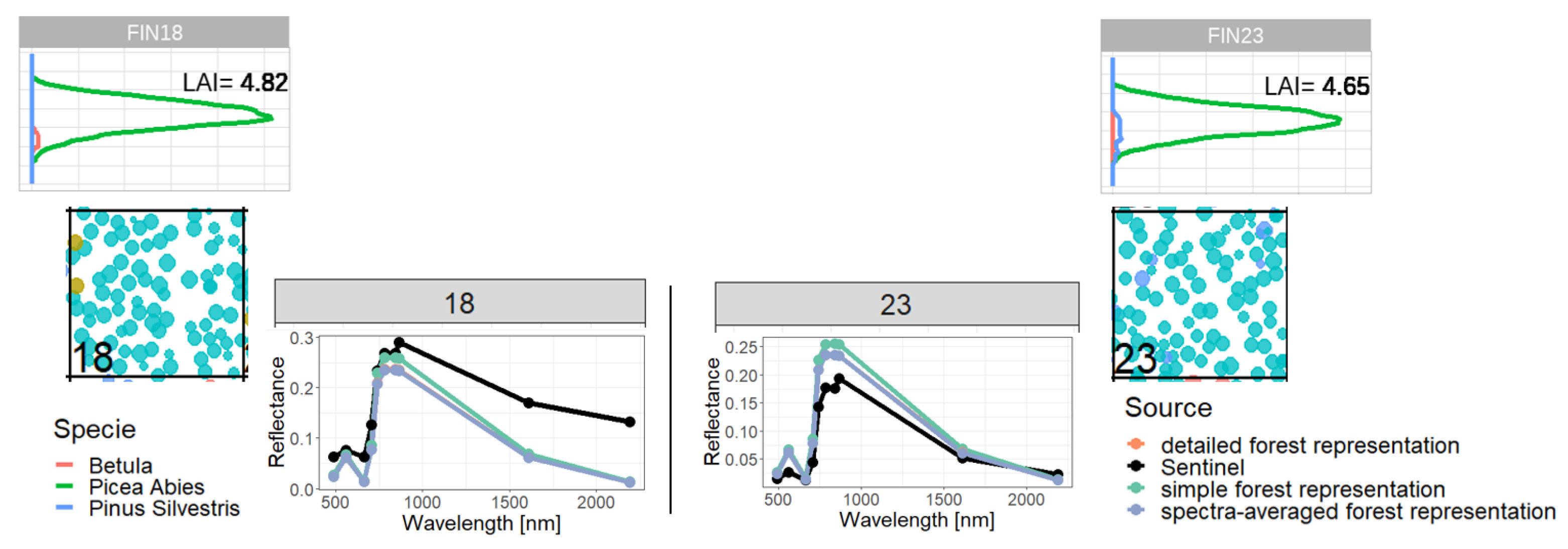
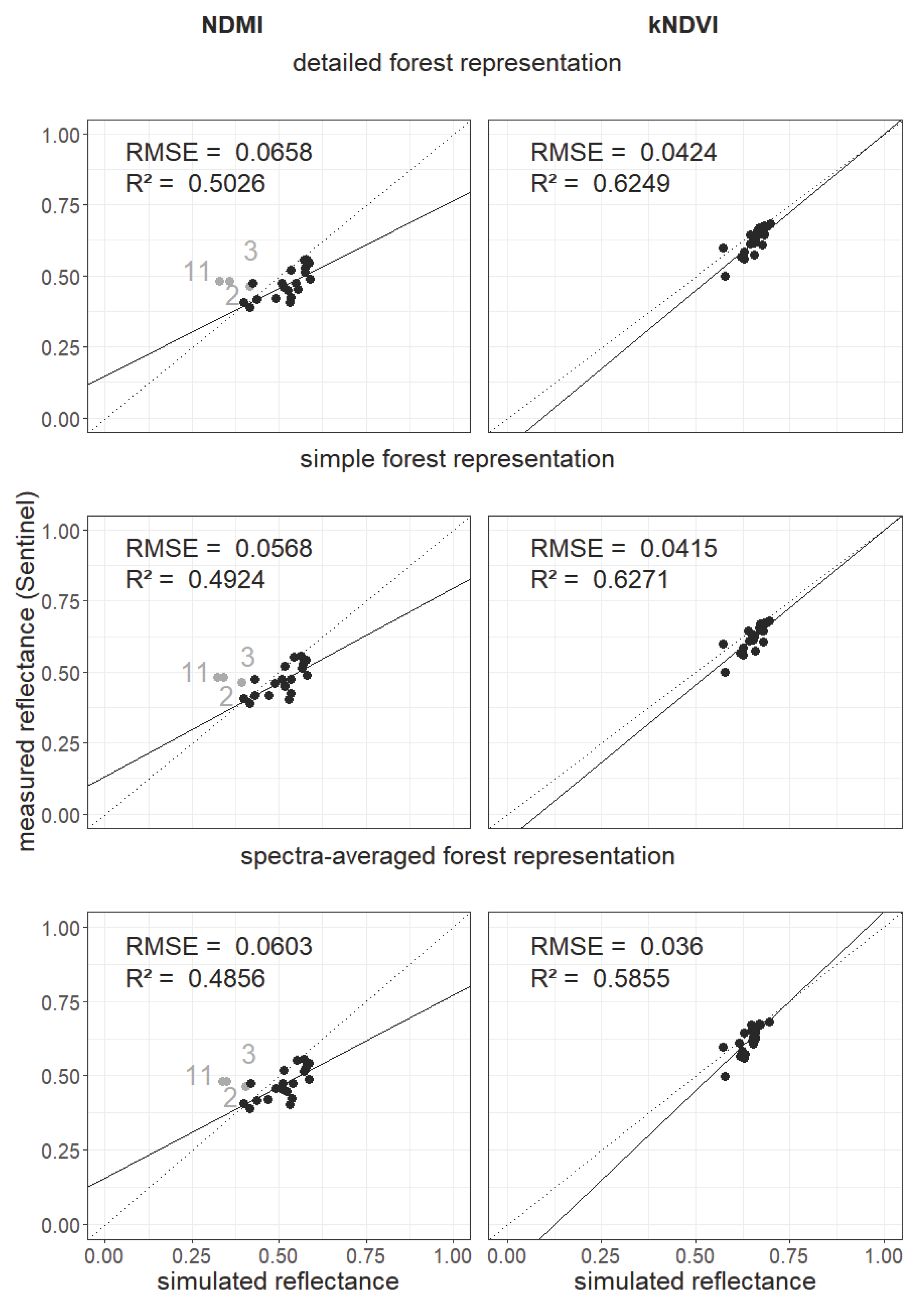
2.4. Representations of Different Levels of Forest Complexity (Heterogeneous Structure)
- 1
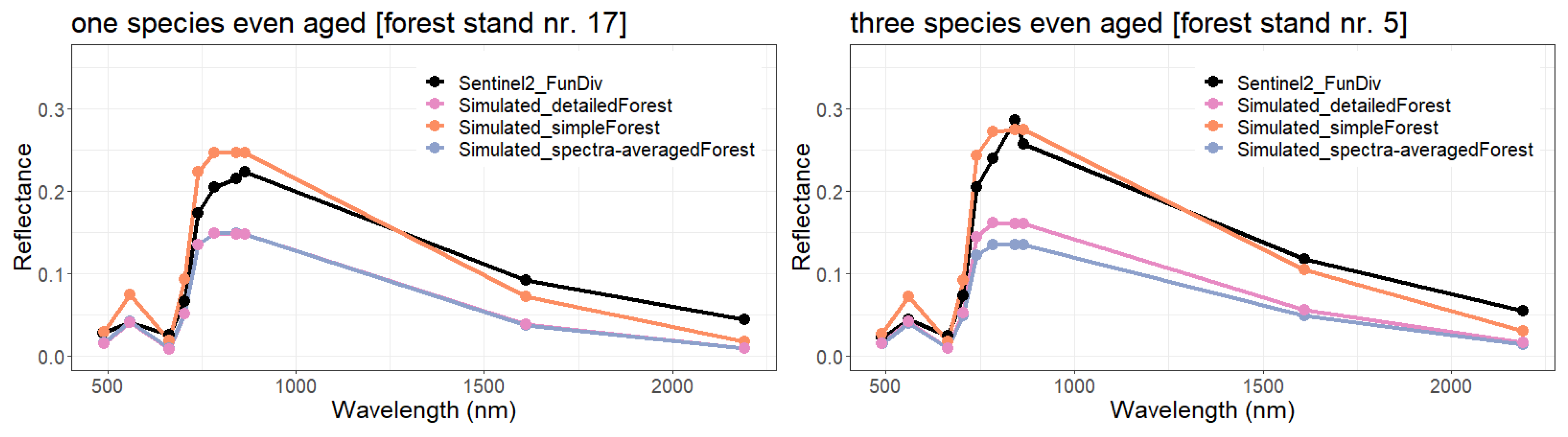
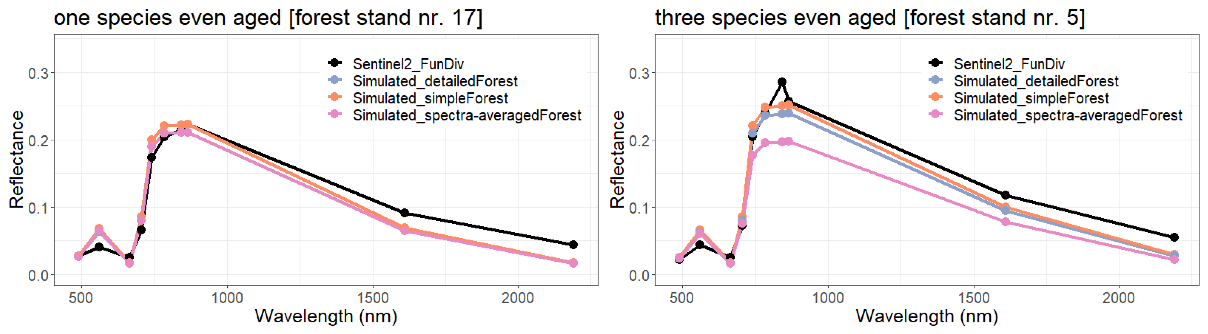
- Simple forest representationThe simplified forest representation only uses reduced information of the forest. It assumes the same mixture of species and the same LAI for each height layer of the forest stand. The leaf parameterization is calculated by averaging the leaf attributes of the occurring species (weighted by LAI, as a measure of abundance). The LAI of the forest stand is equally distributed among all layers.
- 2
- Detailed forest representationThe detailed representation of the forest assigns to each height layer different mixtures of species and different LAIs. The leaf parameterization for each layer is calculated by averaging the leaf attributes of the occurring species weighted by LAI in the height layer, as a measure of abundance. For each layer of the forest, the calculated LAI of the reconstructed forest stand will be used.
- 3
- Spectra-averaged representationIn this case, the forest is divided into different "sub-forests". In each sub-forest stand, we maintain the total number of trees and the structure of the main forest stand. However, we assume that all trees in a sub-forest stand are of only one species. Thus, there are as many sub-forests as there are tree species. For each layer, the calculated LAI of the reconstructed forest stand is used. For each of these single-species sub-forests, the reflectance spectra are calculated using the species-specific leaf parameters. The final reflectance spectrum is determined by averaging the species-specific spectra weighted by LAI fraction, as a measure of abundance.
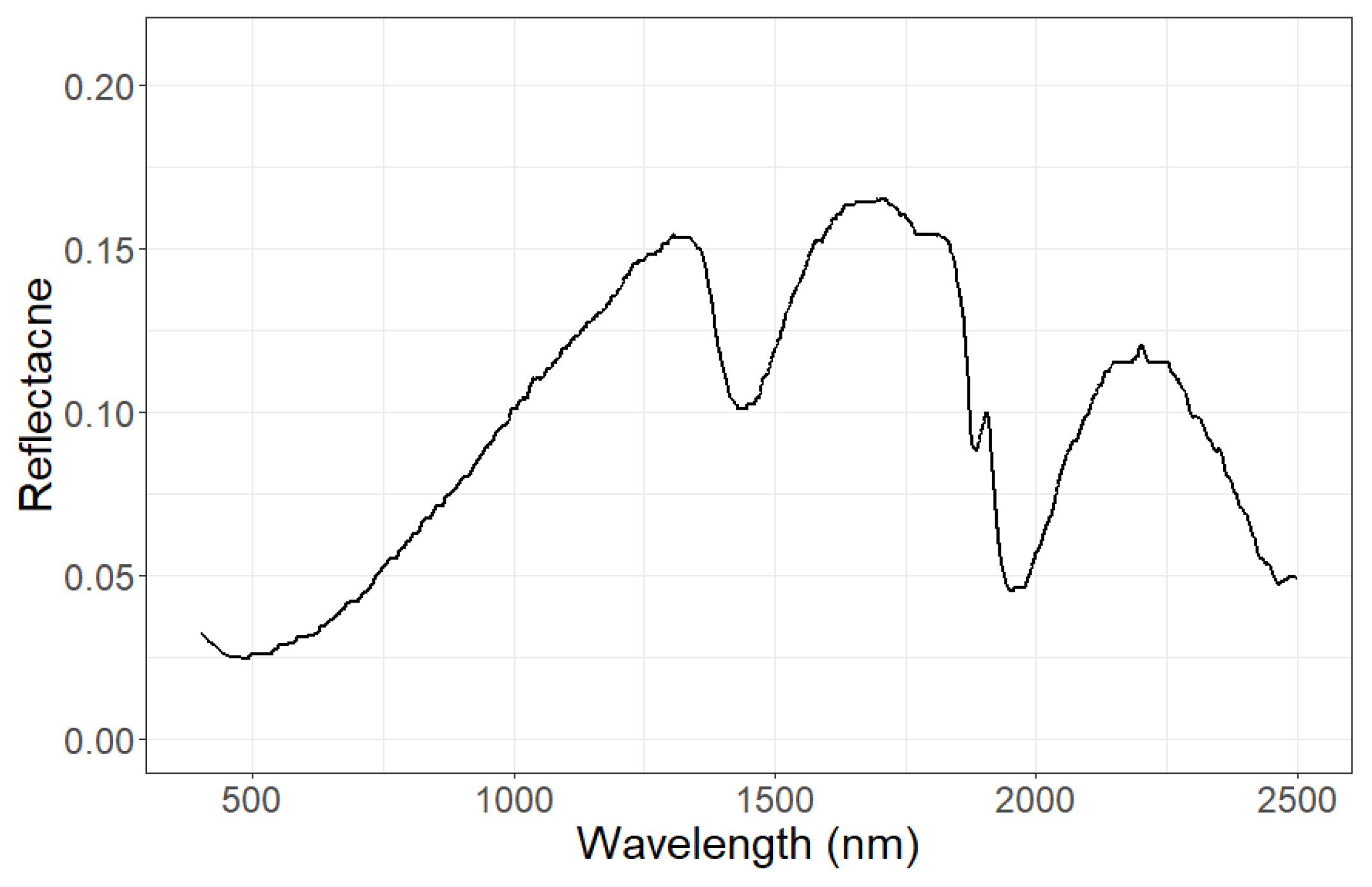
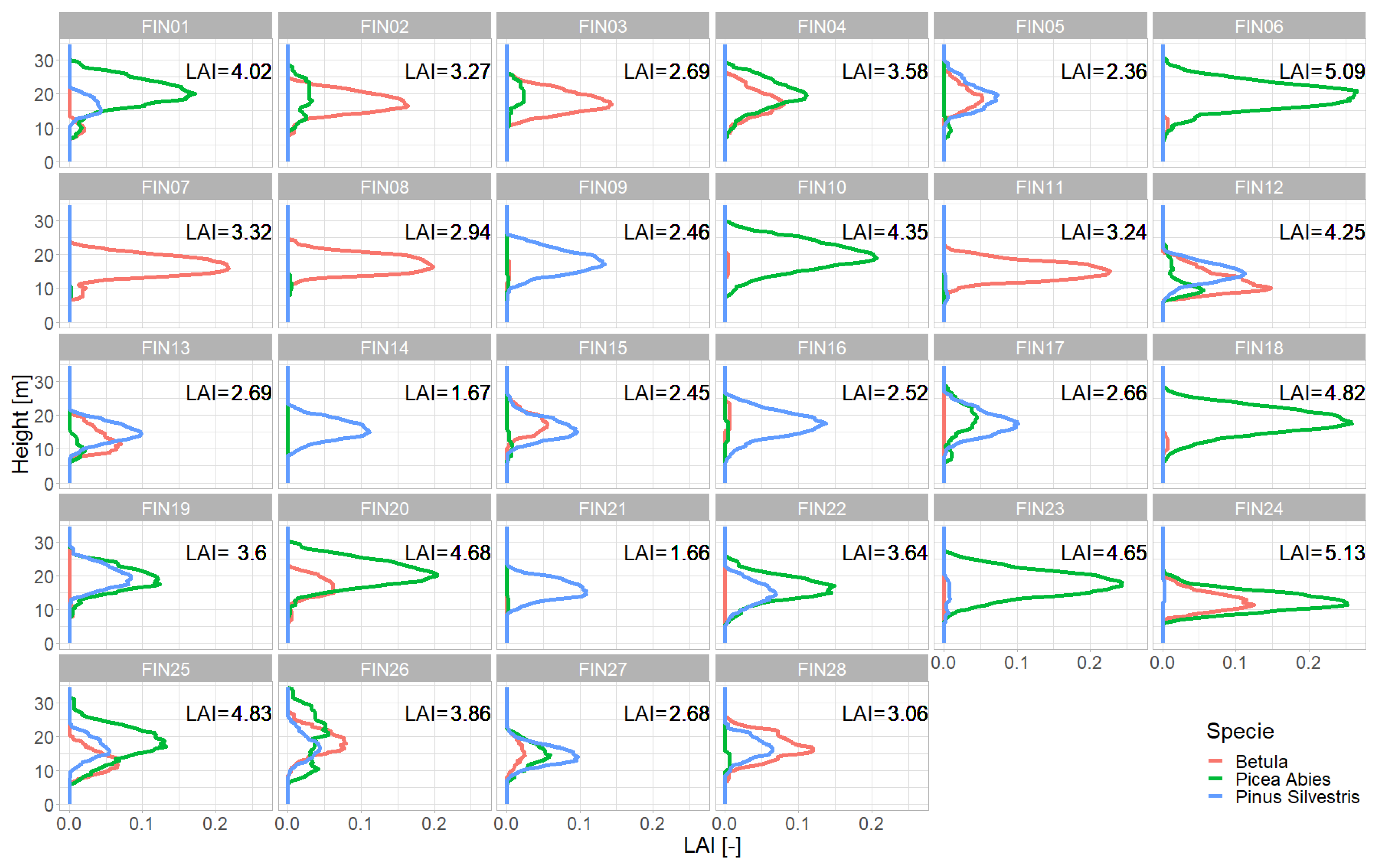
3. Results
4. Discussion
5. Conclusions
Author Contributions
Funding
Institutional Review Board Statement
Informed Consent Statement
Data Availability Statement
Acknowledgments
Conflicts of Interest
Abbreviations
| RTM | Radiative Transfer Model |
| mScope | multilayer Soil Canopy Observation of Photochemistry and Energy fluxes |
| LAI | Leaf Area Index |
| SWIR | Short-Wave Infrared |
| NIRS | Near-Infrared Spectrum |
| RMSE | Root Mean Square Error |
| MAE | Mean Absolute Error |
| NDVI | Normalized Difference Vegetation Index |
| EVI | Enhanced Vegetation Index |
| MSI | Moisture Stress Index |
| NDMI | Normalized Difference Moisture Index |
| kNDVI | kernel NDVI |
| SAD | Spectral Angle Distance |
Appendix A. Additional Information on the Method Section


| Leaf Parameter | Picea Abies | Pinus Silvestrys | Betula (Pendula and Pubescens) |
|---|---|---|---|
| Cab g cm | |||
| Cdm [g cm | |||
| Cw [g cm | |||
| Cs | |||
| Car g cm | |||
| N |
| Plot Number | Basal Area | Maximum Height | Height Heterogeneity | Species Richness | Species Evenness | Biomass | LAI |
|---|---|---|---|---|---|---|---|
| [m ha] | [m] | [m] | [ ha] | ||||
| 1 | 3 | ||||||
| 2 | 19.63 | 28.63 | 3.47 | 2 | 0.35 | 106.83 | 3.23 |
| 3 | 16.31 | 26.38 | 2.88 | 2 | 0.26 | 90.74 | 2.69 |
| 4 | 22.25 | 29.21 | 4.54 | 2 | 0.41 | 118.74 | 3.46 |
| 5 | 19.87 | 29.71 | 4.64 | 5 | 0.74 | 109.47 | 2.26 |
| 6 | 32.84 | 30.80 | 4.04 | 2 | 0.04 | 170.06 | 4.84 |
| 7 | 17.60 | 23.84 | 3.36 | 4 | 0.16 | 94.34 | 3.13 |
| 8 | 17.33 | 24.59 | 2.37 | 3 | 0.17 | 95.09 | 2.94 |
| 9 | 25.66 | 26.10 | 3.69 | 5 | 0.25 | 133.24 | 2.39 |
| 10 | 27.03 | 30.01 | 4.59 | 2 | 0.05 | 139.91 | 3.98 |
| 11 | 17.02 | 22.70 | 2.92 | 3 | 0.27 | 85.02 | 3.15 |
| 12 | 27.35 | 23.32 | 3.39 | 3 | 0.65 | 114.86 | 4.07 |
| 13 | 20.38 | 21.67 | 3.28 | 3 | 0.59 | 88.96 | 2.64 |
| 14 | 18.37 | 23.34 | 2.77 | 1 | 0.00 | 86.37 | 1.67 |
| 15 | 21.37 | 26.22 | 3.38 | 3 | 0.44 | 105.38 | 2.37 |
| 16 | 27.37 | 26.44 | 4.08 | 3 | 0.10 | 139.98 | 2.52 |
| 17 | 24.54 | 28.80 | 4.52 | 2 | 0.38 | 125.61 | 2.58 |
| 18 | 30.99 | 28.45 | 4.24 | 2 | 0.07 | 152.92 | 4.71 |
| 19 | 30.12 | 28.74 | 3.61 | 3 | 0.47 | 162.74 | 3.56 |
| 20 | 30.42 | 30.30 | 3.92 | 2 | 0.35 | 164.55 | 4.52 |
| 21 | 17.60 | 23.34 | 2.45 | 2 | 0.06 | 84.49 | 1.60 |
| 22 | 27.16 | 25.85 | 3.96 | 2 | 0.43 | 120.19 | 3.54 |
| 23 | 29.31 | 27.40 | 4.08 | 2 | 0.16 | 139.35 | 4.44 |
| 24 | 25.45 | 21.70 | 2.63 | 3 | 0.38 | 89.55 | 5.04 |
| 25 | 30.72 | 27.96 | 4.61 | 3 | 0.62 | 145.02 | 4.58 |
| 26 | 26.66 | 34.41 | 5.57 | 4 | 0.69 | 138.13 | 3.67 |
| 27 | 22.03 | 22.77 | 2.95 | 3 | 0.55 | 95.38 | 2.64 |
| 28 | 22.10 | 25.73 | 3.21 | 3 | 0.50 | 114.78 | 2.97 |
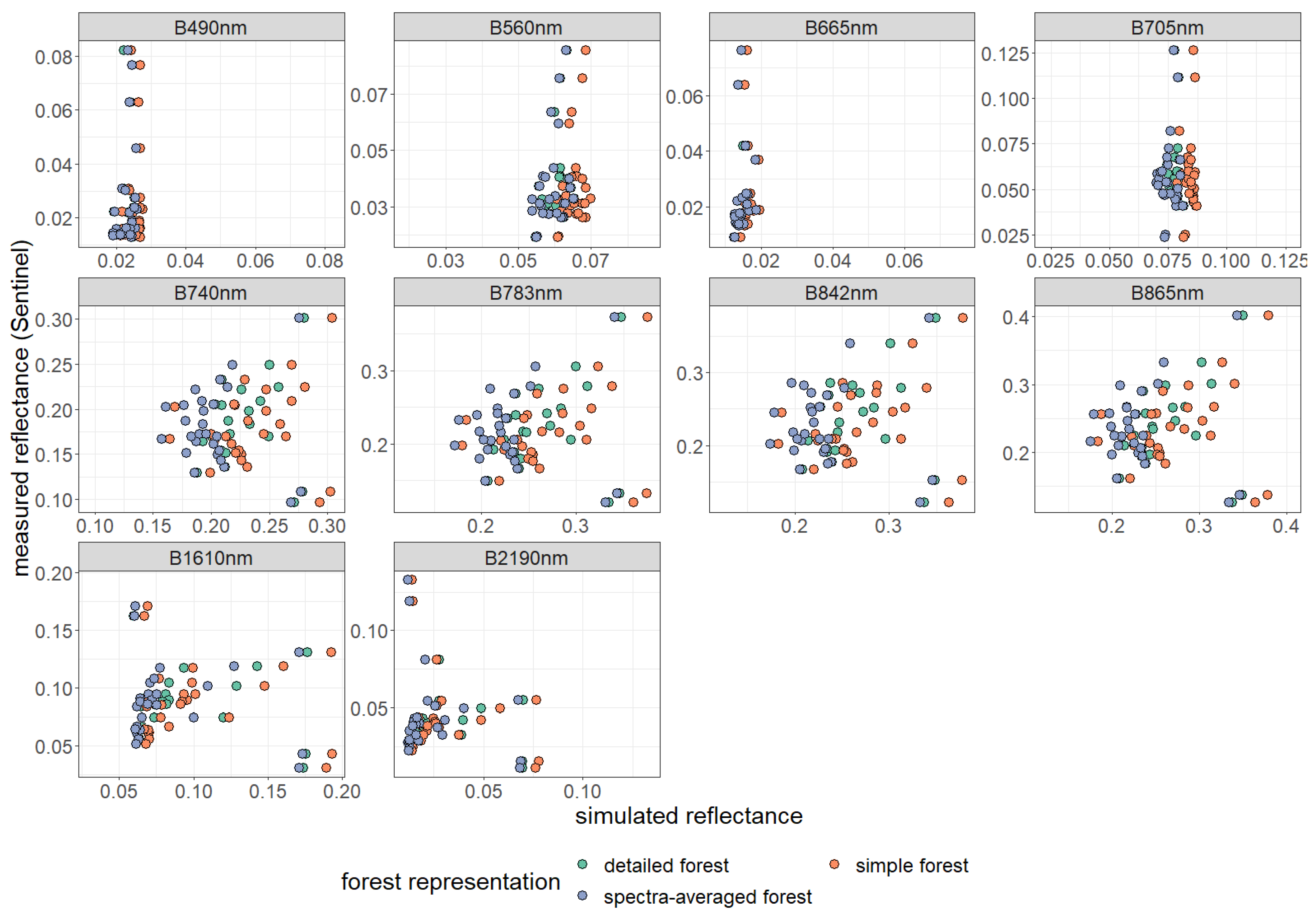
| Spectral Band | Center Wavelength [nm] | Band Name | Band Width [nm] | Spatial Resolution [m] |
|---|---|---|---|---|
| B02 | 490 | blue | 65 | 10 |
| B03 | 560 | green | 35 | 10 |
| B04 | 665 | red | 30 | 10 |
| B05 | 705 | red-edge 1 | 15 | 20 |
| B06 | 740 | red-edge 2 | 15 | 20 |
| B07 | 783 | red-edge 3 | 20 | 20 |
| B08 | 842 | NIR 1 | 115 | 10 |
| B08a | 865 | NIR 2 | 20 | 20 |
| B11 | 1610 | SWIR 1 | 90 | 20 |
| B12 | 2190 | SWIR 2 | 180 | 20 |

Appendix B. Additional Information on the Result Section


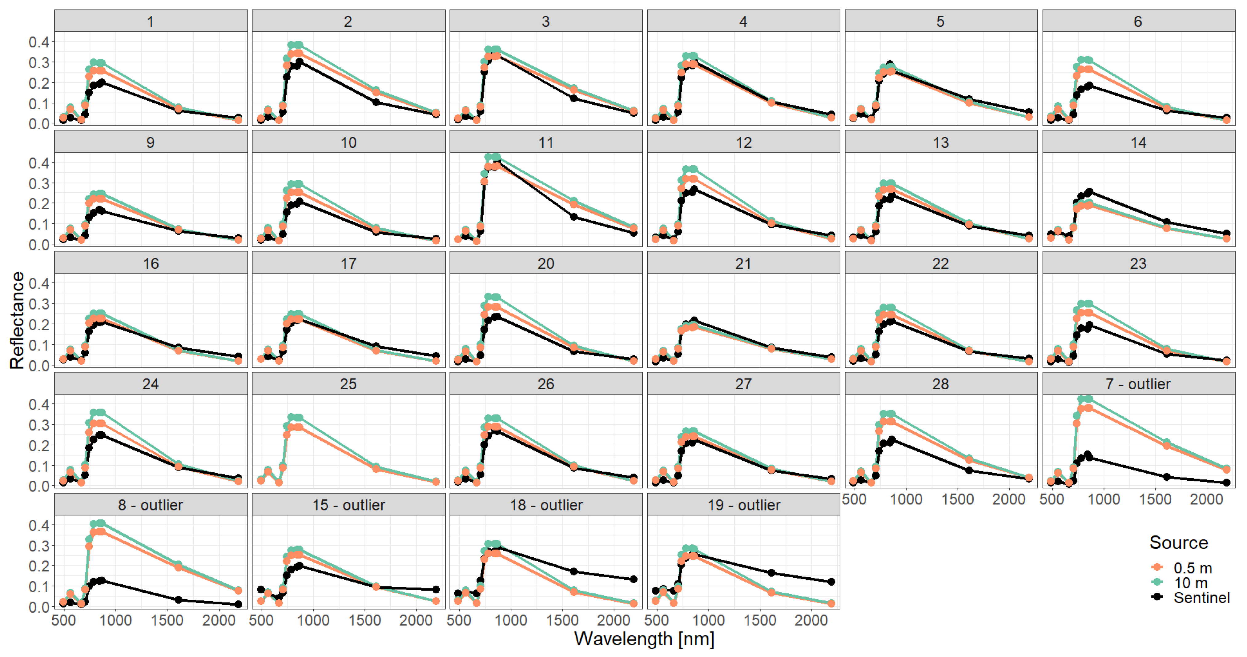
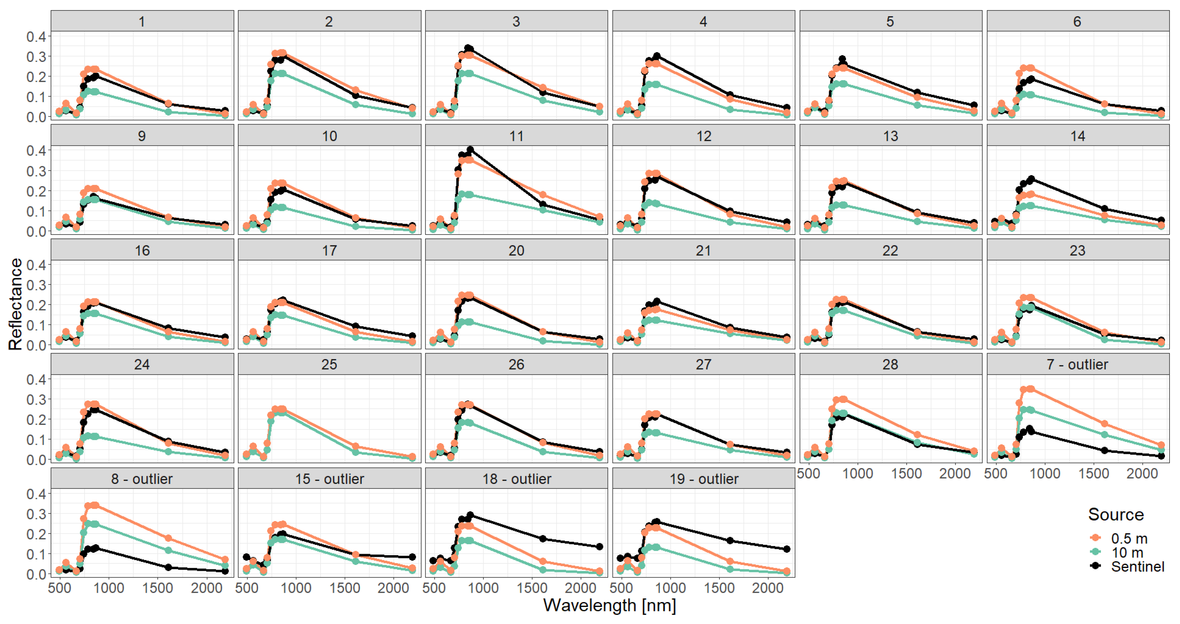
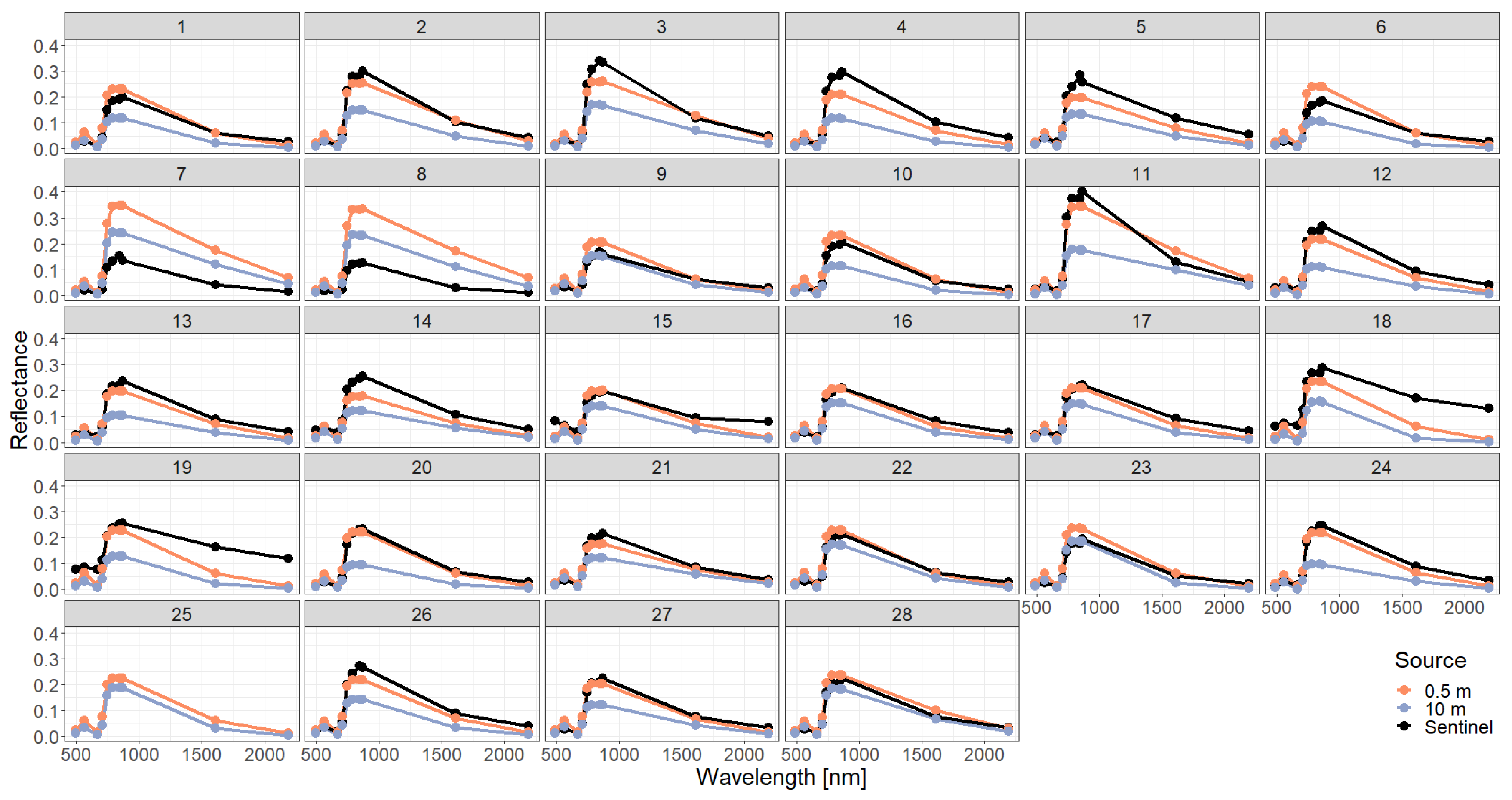
Appendix C. Analysis of Selected Forest Stands (Outliers)


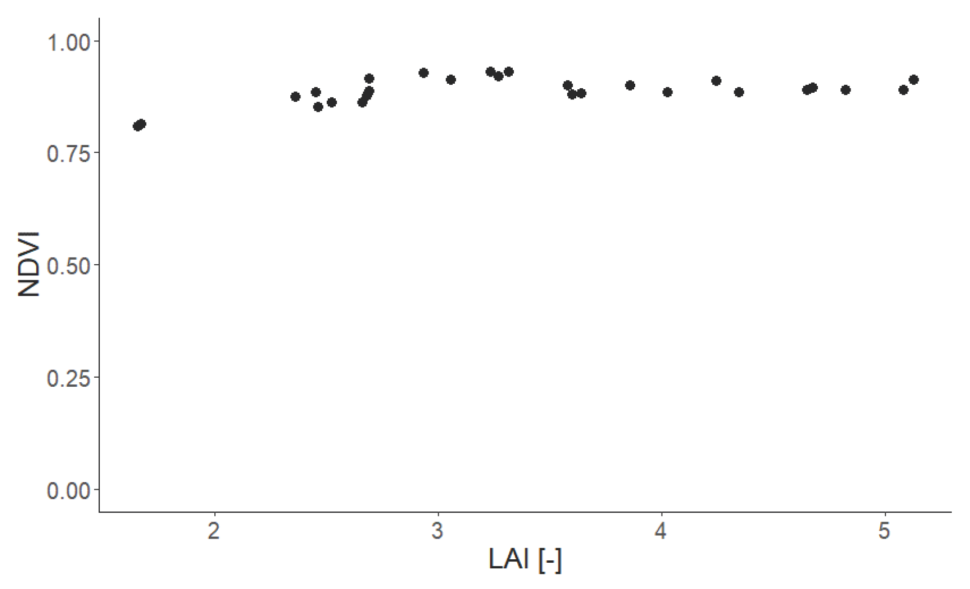
Appendix D. Analysis of LAI and Additional Indices


| Simple Forest | Detailed Forest | Spectra Averaged Forest | |
|---|---|---|---|
| NDVI | |||
| bias | |||
| RMSE | |||
| MAE | |||
| EVI | |||
| bias | |||
| RMSE | |||
| MAE | |||
| MSI | |||
| bias | |||
| RMSE | |||
| MAE | |||
| NDMI | |||
| bias | |||
| RMSE | |||
| MAE | |||
| kNDVI | |||
| bias | |||
| RMSE | |||
| MAE | |||
| mean SAD |
References
- Pan, Y.; Birdsey, R.A.; Fang, J.; Houghton, R.; Kauppi, P.E.; Kurz, W.A.; Phillips, O.L.; Shvidenko, A.; Lewis, S.L.; Canadell, J.G.; et al. A Large and Persistent Carbon Sink in the World’s Forests. Science 2011, 333, 988–993. [Google Scholar] [CrossRef] [PubMed]
- Malhi, Y. The carbon balance of tropical forest regions, 1990–2005. Curr. Opin. Environ. Sustain. 2010, 2, 237–244. [Google Scholar] [CrossRef]
- Ciais, P.; Sabine, C.L.; Bala, G.; Bopp, L.; Brovkin, V.A.; Canadell, J.G.; Chhabra, A.; DeFries, R.S.; Galloway, J.N.; Heimann, M.; et al. Carbon and Other Biogeochemical Cycles. In Climate Change 2013—The Physical Science Basis: Working Group I Contribution to the Fifth Assessment Report of the Intergovernmental Panel on Climate Change; Cambridge University Press: Cambridge, UK, 2014; pp. 465–570. [Google Scholar] [CrossRef]
- FAO. The State of the World’s Forests 2022. Forest Pathways for Green Recovery and Building Inclusive, Resilient and Sustainable Economies; FAO: Rome, Italy, 2022. [Google Scholar] [CrossRef]
- Gibson, L.; Lee, T.M.; Koh, L.P.; Brook, B.W.; Gardner, T.A.; Barlow, J.; Peres, C.A.; Bradshaw, C.J.; Laurance, W.F.; Lovejoy, T.E.; et al. Primary forests are irreplaceable for sustaining tropical biodiversity. Nature 2011, 478, 378–381. [Google Scholar] [CrossRef] [PubMed]
- Myers, N.; Mittermeier, R.A.; Mittermeier, C.G.; Da Fonseca, G.A.; Kent, J. Biodiversity hotspots for conservation priorities. Nature 2000, 403, 853–858. [Google Scholar] [CrossRef]
- Pimm, S.L.; Jenkins, C.N.; Abell, R.; Brooks, T.M.; Gittleman, J.L.; Joppa, L.N.; Raven, P.H.; Roberts, C.M.; Sexton, J.O. The biodiversity of species and their rates of extinction, distribution, and protection. Science 2014, 344, 1246752. [Google Scholar] [CrossRef]
- Pan, Y.; Birdsey, R.A.; Phillips, O.L.; Jackson, R.B. The structure, distribution, and biomass of the world’s forests. Annu. Rev. Ecol. Evol. Syst. 2013, 44, 593–622. [Google Scholar] [CrossRef]
- Guanter, L.; Kaufmann, H.; Segl, K.; Foerster, S.; Rogass, C.; Chabrillat, S.; Kuester, T.; Hollstein, A.; Rossner, G.; Chlebek, C.; et al. The EnMAP spaceborne imaging spectroscopy mission for earth observation. Remote Sens. 2015, 7, 8830–8857. [Google Scholar] [CrossRef]
- Moorcroft, P.R.; Hurtt, G.C.; Pacala, S.W. A method for scaling vegetation dynamics: The ecosystem demography model (ED). Ecol. Monogr. 2001, 71, 557–586. [Google Scholar] [CrossRef]
- Lawrence, D.M.; Oleson, K.W.; Flanner, M.G.; Thornton, P.E.; Swenson, S.C.; Lawrence, P.J.; Zeng, X.; Yang, Z.L.; Levis, S.; Sakaguchi, K.; et al. Parameterization improvements and functional and structural advances in version 4 of the Community Land Model. J. Adv. Model. Earth Syst. 2011, 3, 1–25. [Google Scholar]
- Maréchaux, I.; Langerwisch, F.; Huth, A.; Bugmann, H.; Morin, X.; Reyer, C.P.; Seidl, R.; Collalti, A.; Dantas de Paula, M.; Fischer, R.; et al. Tackling unresolved questions in forest ecology: The past and future role of simulation models. Ecol. Evol. 2021, 11, 3746–3770. [Google Scholar] [CrossRef]
- Shugart, H.H.; Wang, B.; Fischer, R.; Ma, J.; Fang, J.; Yan, X.; Huth, A.; Armstrong, A.H. Gap models and their individual-based relatives in the assessment of the consequences of global change. Environ. Res. Lett. 2018, 13, 033001. [Google Scholar] [CrossRef]
- Köhler, P.; Huth, A. The effects of tree species grouping in tropical rainforest modelling: Simulations with the individual-based model Formind. Ecol. Model. 1998, 109, 301–321. [Google Scholar] [CrossRef]
- Smith, B. LPJ-GUESS-An Ecosystem Modelling Framework; Department of Physical Geography and Ecosystems Analysis, INES, Sölvegatan: Lund, Sweden, 2001; Volume 12, p. 22362. [Google Scholar]
- Sellers, P.J. Canopy reflectance, photosynthesis and transpiration. Int. J. Remote Sens. 1985, 6, 1335–1372. [Google Scholar] [CrossRef]
- Kokhanovsky, A.A.; Kuusk, A.; Lang, M.; Kuusk, J. Database of optical and structural data for the validation of forest radiative transfer models. In Light Scattering Reviews 7: Radiative Transfer and Optical Properties of Atmosphere and Underlying Surface; Springer: Berlin/Heidelberg, Germany, 2013; pp. 109–148. [Google Scholar]
- Kuusk, A. Canopy Radiative Transfer Modeling. In Comprehensive Remote Sensing; Liang, S., Ed.; Elsevier: Oxford, UK, 2018; pp. 9–22. [Google Scholar] [CrossRef]
- Brazhnik, K.; Shugart, H. Model sensitivity to spatial resolution and explicit light representation for simulation of boreal forests in complex terrain. Ecol. Model. 2017, 352, 90–107. [Google Scholar] [CrossRef]
- Deutschmann, T.; Beirle, S.; Frieß, U.; Grzegorski, M.; Kern, C.; Kritten, L.; Platt, U.; Prados-Román, C.; Puķı, J.; Wagner, T.; et al. The Monte Carlo atmospheric radiative transfer model McArtim: Introduction and validation of Jacobians and 3D features. J. Quant. Spectrosc. Radiat. Transf. 2011, 112, 1119–1137. [Google Scholar] [CrossRef]
- Verhoef, W.; Jia, L.; Xiao, Q.; Su, Z. Unified optical-thermal four-stream radiative transfer theory for homogeneous vegetation canopies. IEEE Trans. Geosci. Remote Sens. 2007, 45, 1808–1822. [Google Scholar] [CrossRef]
- Bonan, G.B.; Lawrence, P.J.; Oleson, K.W.; Levis, S.; Jung, M.; Reichstein, M.; Lawrence, D.M.; Swenson, S.C. Improving canopy processes in the Community Land Model version 4 (CLM4) using global flux fields empirically inferred from FLUXNET data. J. Geophys. Res. Biogeosci. 2011, 116, G02014. [Google Scholar] [CrossRef]
- Medvigy, D.; Wofsy, S.; Munger, J.; Hollinger, D.; Moorcroft, P. Mechanistic scaling of ecosystem function and dynamics in space and time: Ecosystem Demography model version 2. J. Geophys. Res. Biogeosci. 2009, 114, G01002. [Google Scholar] [CrossRef]
- Bonan, G.; Williams, M.; Fisher, R.; Oleson, K. Modeling stomatal conductance in the earth system: Linking leaf water-use efficiency and water transport along the soil–plant–atmosphere continuum. Geosci. Model Dev. 2014, 7, 2193–2222. [Google Scholar] [CrossRef]
- Gastellu-Etchegorry, J.P.; Lauret, N.; Yin, T.; Landier, L.; Kallel, A.; Malenovský, Z.; Bitar, A.A.; Aval, J.; Benhmida, S.; Qi, J.; et al. DART: Recent Advances in Remote Sensing Data Modeling With Atmosphere, Polarization, and Chlorophyll Fluorescence. IEEE J. Sel. Top. Appl. Earth Obs. Remote Sens. 2017, 10, 2640–2649. [Google Scholar] [CrossRef]
- Yang, P.; Verhoef, W.; van der Tol, C. The mSCOPE model: A simple adaption to the SCOPE model to describe reflectance, fluorescence and photosynthesis of vertically heterogeneous canopies. Remote Control. Environ. 2017, 201, 1–11. [Google Scholar] [CrossRef]
- Baeten, L.; Verheyen, K.; Wirth, C.; Bruelheide, H.; Bussotti, F.; Finér, L.; Jaroszewicz, B.; Selvi, F.; Valladares, F.; Allan, E.; et al. A novel comparative research platform designed to determine the functional significance of tree species diversity in European forests. Perspect. Plant Ecol. Evol. Syst. 2013, 15, 281–291. [Google Scholar] [CrossRef]
- Ma, X.; Mahecha, M.D.; Migliavacca, M.; van der Plas, F.; Benavides, R.; Ratcliffe, S.; Kattge, J.; Richter, R.; Musavi, T.; Baeten, L.; et al. Inferring plant functional diversity from space: The potential of Sentinel-2. Remote Sens. Environ. 2019, 233, 111368. [Google Scholar] [CrossRef]
- Paulick, S.; Dislich, C.; Homeier, J.; Fischer, R.; Huth, A. The carbon fluxes in different successional stages: Modelling the dynamics of tropical montane forests in South Ecuador. For. Ecosyst. 2017, 4, 1–11. [Google Scholar] [CrossRef]
- Rödig, E.; Cuntz, M.; Rammig, A.; Fischer, R.; Taubert, F.; Huth, A. The importance of forest structure for carbon fluxes of the Amazon rainforest. Environ. Res. Lett. 2018, 13, 054013. [Google Scholar] [CrossRef]
- Köhler, P.; Huth, A. Simulating growth dynamics in a South-East Asian rainforest threatened by recruitment shortage and tree harvesting. Clim. Chang. 2004, 67, 95–117. [Google Scholar] [CrossRef]
- Gutiérrez, A.G.; Huth, A. Successional stages of primary temperate rainforests of Chiloé Island, Chile. Perspect. Plant Ecol. Evol. Syst. 2012, 14, 243–256. [Google Scholar] [CrossRef]
- Huth, A.; Ditzer, T. Long-term impacts of logging in a tropical rain forest—A simulation study. For. Ecol. Manag. 2001, 142, 33–51. [Google Scholar] [CrossRef]
- Kammesheidt, L.; Köhler, P.; Huth, A. Sustainable timber harvesting in Venezuela: A modelling approach. J. Appl. Ecol. 2001, 38, 756–770. [Google Scholar] [CrossRef]
- Köhler, P.; Chave, J.; Riéra, B.; Huth, A. Simulating the long-term response of tropical wet forests to fragmentation. Ecosystems 2003, 6, 114–128. [Google Scholar] [CrossRef]
- Köhler, P.; Huth, A. Impacts of recruitment limitation and canopy disturbance on tropical tree species richness. Ecol. Model. 2007, 203, 511–517. [Google Scholar] [CrossRef]
- Rüger, N.; Williams-Linera, G.; Kissling, W.D.; Huth, A. Long-term impacts of fuelwood extraction on a tropical montane cloud forest. Ecosystems 2008, 11, 868–881. [Google Scholar] [CrossRef]
- Fischer, R.; Armstrong, A.; Shugart, H.H.; Huth, A. Simulating the impacts of reduced rainfall on carbon stocks and net ecosystem exchange in a tropical forest. Environ. Model. Softw. 2014, 52, 200–206. [Google Scholar] [CrossRef]
- Bohn, F.J.; Frank, K.; Huth, A. Of climate and its resulting tree growth: Simulating the productivity of temperate forests. Ecol. Model. 2014, 278, 9–17. [Google Scholar] [CrossRef]
- Bruening, J.M.; Fischer, R.; Bohn, F.J.; Armston, J.; Armstrong, A.H.; Knapp, N.; Tang, H.; Huth, A.; Dubayah, R. Challenges to aboveground biomass prediction from waveform lidar. Environ. Res. Lett. 2021, 16, 125013. [Google Scholar] [CrossRef]
- Rüger, N.; Gutiérrez, A.G.; Kissling, W.D.; Armesto, J.J.; Huth, A. Ecological impacts of different harvesting scenarios for temperate evergreen rain forest in southern Chile—A simulation experiment. For. Ecol. Manag. 2007, 252, 52–66. [Google Scholar] [CrossRef]
- Taubert, F.; Frank, K.; Huth, A. A review of grassland models in the biofuel context. Ecol. Model. 2012, 245, 84–93. [Google Scholar] [CrossRef]
- Reyer, C.P.O.; Silveyra Gonzalez, R.; Dolos, K.; Hartig, F.; Hauf, Y.; Noack, M.; Lasch-Born, P.; Rötzer, T.; Pretzsch, H.; Meesenburg, H.; et al. The PROFOUND Database for evaluating vegetation models and simulating climate impacts on European forests. Earth Syst. Sci. Data 2020, 12, 1295–1320. [Google Scholar] [CrossRef]
- van der Tol, C.; Verhoef, W.; Timmermans, J.; Verhoef, A.; Su, Z. An integrated model of soil-canopy spectral radiances, photosynthesis, fluorescence, temperature and energy balance. Biogeosciences 2009, 6, 3109–3129. [Google Scholar] [CrossRef]
- Vilfan, N.; van der Tol, C.; Muller, O.; Rascher, U.; Verhoef, W. Fluspect-B: A model for leaf fluorescence, reflectance and transmittance spectra. Remote Sens. Environ. 2016, 186, 596–615. [Google Scholar] [CrossRef]
- Féret, J.B.; Gitelson, A.; Noble, S.; Jacquemoud, S. PROSPECT-D: Towards modeling leaf optical properties through a complete lifecycle. Remote Sens. Environ. 2017, 193, 204–215. [Google Scholar] [CrossRef]
- Verhoef, W. Light scattering by leaf layers with application to canopy reflectance modeling: The SAIL model. Remote Sens. Environ. 1984, 16, 125–141. [Google Scholar] [CrossRef]
- Kothari, S.; Beauchamp-Rioux, R.; Blanchard, F.; Crofts, A.L.; Girard, A.; Guilbeault-Mayers, X.; Hacker, P.W.; Pardo, J.; Schweiger, A.K.; Demers-Thibeault, S.; et al. Predicting leaf traits across functional groups using reflectance spectroscopy. New Phytol. 2023, 238, 549–566. [Google Scholar] [CrossRef] [PubMed]
- Huete, A.; Didan, K.; Miura, T.; Rodriguez, E.P.; Gao, X.; Ferreira, L.G. Overview of the radiometric and biophysical performance of the MODIS vegetation indices. Remote Sens. Environ. 2002, 83, 195–213. [Google Scholar] [CrossRef]
- Gao, X.; Huete, A.R.; Ni, W.; Miura, T. Optical–biophysical relationships of vegetation spectra without background contamination. Remote Sens. Environ. 2000, 74, 609–620. [Google Scholar] [CrossRef]
- Camps-Valls, G.; Campos-Taberner, M.; Moreno-Martínez, Á.; Walther, S.; Duveiller, G.; Cescatti, A.; Mahecha, M.D.; Muñoz-Marí, J.; García-Haro, F.J.; Guanter, L.; et al. A unified vegetation index for quantifying the terrestrial biosphere. Sci. Adv. 2021, 7, eabc7447. [Google Scholar] [CrossRef]
- Hardisky, M.H.; Klemas, V.; Smart, R. The influence of soil salinity, growth form, and leaf moisture on-the spectral radiance of Spartina alterniflora Canopies. Photogramm. Eng. Remote Sens. 1983, 49, 77–83. [Google Scholar]
- Hunt Jr, E.R.; Rock, B.N. Detection of changes in leaf water content using near-and middle-infrared reflectances. Remote Sens. Environ. 1989, 30, 43–54. [Google Scholar] [CrossRef]
- Vogelmann, J.; Rock, B. Assessing forest decline in coniferous forests of Vermont using NS-001 Thematic Mapper Simulator data. Int. J. Remote Sens. 1986, 7, 1303–1321. [Google Scholar] [CrossRef]
- Kruse, F.A.; Lefkoff, A.; Boardman, J.; Heidebrecht, K.; Shapiro, A.; Barloon, P.; Goetz, A. The spectral image processing system (SIPS)—Interactive visualization and analysis of imaging spectrometer data. Remote Sens. Environ. 1993, 44, 145–163. [Google Scholar] [CrossRef]
- Huete, A.R.; Liu, H.; Batchily, K.; van Leeuwen, W. A comparison of vegetation indices over a global set of TM images for EOS-MODIS. Remote Sens. Environ. 1997, 59, 440–451. [Google Scholar] [CrossRef]
- Bussotti, F.; Pollastrini, M. Evaluation of leaf features in forest trees: Methods, techniques, obtainable information and limits. Ecol. Indic. 2015, 52, 219–230. [Google Scholar] [CrossRef]
- Jacquemoud, S.; Ustin, S. Leaf Optical Properties; Cambridge University Press: Cambridge, UK, 2019. [Google Scholar]
- Kattenborn, T.; Fassnacht, F.E.; Schmidtlein, S. Differentiating plant functional types using reflectance: Which traits make the difference? Remote Sens. Ecol. Conserv. 2019, 5, 5–19. [Google Scholar] [CrossRef]
- Kattenborn, T.; Richter, R.; Guimarães-Steinicke, C.; Feilhauer, H.; Wirth, C. AngleCam: Predicting the temporal variation of leaf angle distributions from image series with deep learning. Methods Ecol. Evol. 2022, 13, 2531–2545. [Google Scholar] [CrossRef]
- Jacquemoud, S.; Verhoef, W.; Baret, F.; Bacour, C.; Zarco-Tejada, P.J.; Asner, G.P.; François, C.; Ustin, S.L. PROSPECT+ SAIL models: A review of use for vegetation characterization. Remote Sens. Environ. 2009, 113, S56–S66. [Google Scholar] [CrossRef]
- Verhoef, W.; Van Der Tol, C.; Middleton, E.M. Hyperspectral radiative transfer modeling to explore the combined retrieval of biophysical parameters and canopy fluorescence from FLEX–Sentinel-3 tandem mission multi-sensor data. Remote Sens. Environ. 2018, 204, 942–963. [Google Scholar] [CrossRef]
- Rödig, E.; Knapp, N.; Fischer, R.; Bohn, F.J.; Dubayah, R.; Tang, H.; Huth, A. From small-scale forest structure to Amazon-wide carbon estimates. Nat. Commun. 2019, 10, 5088. [Google Scholar] [CrossRef]
- Henniger, H.; Huth, A.; Frank, K.; Bohn, F. Creating virtual forest around the globe: Forest Factory 2.0 and analysing the state space of forests. Ecol. Model. 2023. [Google Scholar] [CrossRef]
- Bohn, F.J.; Huth, A. The importance of forest structure to biodiversity–productivity relationships. R. Soc. Open Sci. 2017, 4, 160521. [Google Scholar] [CrossRef]
- Pacheco-Labrador, J.; Perez-Priego, O.; El-Madany, T.S.; Julitta, T.; Rossini, M.; Guan, J.; Moreno, G.; Carvalhais, N.; Martín, M.P.; Gonzalez-Cascon, R.; et al. Multiple-constraint inversion of SCOPE. Evaluating the potential of GPP and SIF for the retrieval of plant functional traits. Remote Sens. Environ. 2019, 234, 111362. [Google Scholar] [CrossRef]
- Fischer, R.; Bohn, F.; Dantas de Paula, M.; Dislich, C.; Groeneveld, J.; Gutiérrez, A.G.; Kazmierczak, M.; Knapp, N.; Lehmann, S.; Paulick, S.; et al. Lessons learned from applying a forest gap model to understand ecosystem and carbon dynamics of complex tropical forests. Ecol. Model. 2016, 326, 124–133. [Google Scholar] [CrossRef]


Disclaimer/Publisher’s Note: The statements, opinions and data contained in all publications are solely those of the individual author(s) and contributor(s) and not of MDPI and/or the editor(s). MDPI and/or the editor(s) disclaim responsibility for any injury to people or property resulting from any ideas, methods, instructions or products referred to in the content. |
© 2023 by the authors. Licensee MDPI, Basel, Switzerland. This article is an open access article distributed under the terms and conditions of the Creative Commons Attribution (CC BY) license (https://creativecommons.org/licenses/by/4.0/).
Share and Cite
Henniger, H.; Bohn, F.J.; Schmidt, K.; Huth, A. A New Approach Combining a Multilayer Radiative Transfer Model with an Individual-Based Forest Model: Application to Boreal Forests in Finland. Remote Sens. 2023, 15, 3078. https://doi.org/10.3390/rs15123078
Henniger H, Bohn FJ, Schmidt K, Huth A. A New Approach Combining a Multilayer Radiative Transfer Model with an Individual-Based Forest Model: Application to Boreal Forests in Finland. Remote Sensing. 2023; 15(12):3078. https://doi.org/10.3390/rs15123078
Chicago/Turabian StyleHenniger, Hans, Friedrich J. Bohn, Kim Schmidt, and Andreas Huth. 2023. "A New Approach Combining a Multilayer Radiative Transfer Model with an Individual-Based Forest Model: Application to Boreal Forests in Finland" Remote Sensing 15, no. 12: 3078. https://doi.org/10.3390/rs15123078
APA StyleHenniger, H., Bohn, F. J., Schmidt, K., & Huth, A. (2023). A New Approach Combining a Multilayer Radiative Transfer Model with an Individual-Based Forest Model: Application to Boreal Forests in Finland. Remote Sensing, 15(12), 3078. https://doi.org/10.3390/rs15123078