Article

Integrating Remote Sensing and Weather Variables for Mango Yield Prediction Using a Machine Learning Approach

by
Benjamin Adjah Torgbor
*,
Muhammad Moshiur Rahman
,
James Brinkhoff
,
Priyakant Sinha
and
Andrew Robson
Applied Agricultural Remote Sensing Centre, University of New England, Armidale, NSW 2351, Australia
*
Author to whom correspondence should be addressed.
Remote Sens. 2023, 15(12), 3075; https://doi.org/10.3390/rs15123075
Submission received: 28 April 2023 / Revised: 5 June 2023 / Accepted: 10 June 2023 / Published: 12 June 2023

Abstract

:
Accurate pre-harvest yield forecasting of mango is essential to the industry as it supports better decision making around harvesting logistics and forward selling, thus optimizing productivity and reducing food waste. Current methods for yield forecasting such as manually counting 2–3% of the orchard can be accurate but are very time inefficient and labour intensive. More recent evaluations of technological solutions such as remote (satellite) and proximal (on ground) sensing have provided very encouraging results, but they still require infield in-season sampling for calibration, the technology comes at a significant cost, and commercial availability is limited, especially for vehicle-mounted sensors. This study presents the first evaluation of a ”time series”—based remote sensing method for yield forecasting of mango, a method that does not require infield fruit counts and utilizes freely available satellite imagery. Historic yield data from 2015 to 2022 were sourced from 51 individual orchard blocks from two farms (AH and MK) in the Northern Territory of Australia. Time series measures of the canopy reflectance properties of the blocks were obtained from Landsat 7 and 8 satellite data for the 2015–2022 growing seasons. From the imagery, the following vegetation indices (VIs) were derived: EVI, GNDVI, NDVI, and LSWI, whilst corresponding weather variables (rainfall (Prec), temperature (Tmin/Tmax), evapotranspiration (ETo), solar radiation (Rad), and vapor pressure deficit (vpd)) were also sourced from SILO data. To determine the relationships among weather and remotely sensed measures of canopy throughout the growing season and the yield achieved (at the block level and the farm level), six machine learning (ML) algorithms, namely random forest (RF), support vector regression (SVR), eXtreme gradient boosting (XGBOOST), RIDGE, LASSO and partial least square regression (PLSR), were trialed. The EVI/GNDVI and Prec/Tmin were found to be the best RS and weather predictors, respectively. The block-level combined RS/weather-based RF model for 2021 produced the best result (MAE = 2.9 t/ha), marginally better than the RS only RF model (MAE = 3.4 t/ha). The farm-level model error (FLEM) was generally lower than the block-level model error, for both the combined RS/weather-based RF model (farm = 3.7%, block (NMAE) = 33.6% for 2021) and the RS-based model (farm = 4.3%, block = 38.4% for 2021). Further testing of the RS/weather-based RF models over six additional orchards (other than AH and MK) produced errors ranging between 24% and 39% from 2016 to 2020. Although accuracies of prediction did vary at both the block level and the farm level, this preliminary study demonstrates the potential of a ”time series” RS method for predicting mango yields. The benefits to the mango industry are that it utilizes freely available imagery, requires no infield calibration, and provides predictions several months before the commercial harvest. Therefore, this outcome not only presents a more adoptable option for the industry, but also better supports automation and scalability in terms of block-, farm-, regional, and national level forecasting.

1. Introduction

The global production of mango (Mangifera indica) has been consistently increasing since the early 1960s [1,2]. According to the Food and Agricultural Organization (FAO) of the United Nations, global production increased from 10.9 million tons in 1961 to over 57 million tons in 2021, representing a 422% increase [1]. In terms of export value, mango’s contribution to the global economy rose from USD 0.6 million to approximately USD 3.7 billion from 1961 to 2021, respectively [1]. In Australia, mango production is on the rise with over 50% of the production, by volume and value within the economy, contributed by growers in the Northern Territory (NT) alone. For the 2020/2021 season, the region’s contribution was estimated at AUD 128 million (USD 88.4 million) [3,4,5].
Currently, the mango industry lacks access to reliable pre-harvest yield prediction technologies, and therefore growers and the greater industry struggle with harvesting logistics (labor, transport, storage, and processing requirements) as well as total production estimates to support forward selling [6,7]. This often results in wastage of fruits causing financial loss to growers and eventually affecting the contribution of the mango industry to the economy of growing nations. Furthermore, at the farm level, accurate yield prediction promotes efficient use of farm inputs and resources such as irrigation, fertilizer, labor, and machinery [8,9]. Additionally, understanding the spatial variability in yield across the farm, growers are able to optimize production by focusing on low yielding blocks to match high yielding blocks or to plan fertilization and other management programs in the lower yield areas. There is, therefore, the need for a technology that predicts annual yield several months ahead of the commencement of the harvesting season.
Physical-based methods such as individual fruit counts of trees are the most commonly used commercial practice for yield estimation. More recently, machine vision and other in-season yield estimation approaches have been investigated [10]. However, such approaches are often expensive and limited in terms of scale [11]. Additionally, those methods are often labor intensive and yield estimates are obtained late in the season [12]. The proliferation of different satellite remote sensing platforms in recent times, offering sensors of varying resolutions (i.e., radiometric, spatial, spectral, and temporal) have opened the possibility of characterizing crop yield at varying spatio-temporal scales. Particularly, the availability of the free data from platforms with moderate to high resolution sensors that offer frequent revisit, such as Landsat and Sentinel-2, coupled with advanced statistical and ML methods have made yield prediction studies more impactful at the block level and the farm level [13,14]. Although numerous studies have produced interesting results using linear parametric statistical models, new and advanced non-parametric ML approaches have revolutionized the yield prediction space, capturing the nonlinear and complex relationships among yield and predictor variables [15,16,17,18]. Statistical models have focused on building empirical predictive algorithms based on multi-source historical data. They have the ability to predict yield independently of the physiological processes that define plants’ growth inter alia, without reliance on individual crop specific parameters such as with mechanistic models [6]. Statistical models have been widely used with remotely sensed VIs to predict yield of fruit trees such as macadamia, mango, avocado, citrus, and peach [9,19,20,21,22] due to the relative ease in its application compared to process-based models.
A number of studies have looked at yield estimation and prediction of different fruit crops using different remote sensing platforms with varying accuracies [19,23,24]. In a study conducted in Italy, Matese and Di Gennaro [15] predicted grape yield using the Gaussian process regression method on the normalized difference vegetation index (NDVI), canopy thickness, and canopy volume to achieve over 85% accuracy and an R2 value of 0.80. Bai et al. [25] used a random forest (RF) model to predict apple yield with an RMSE of 19.9 kg·tree−1 and R2 of 0.71. Additionally, Rahman et al. [9] predicted mango yield per tree using an artificial neural network (ANN) model that combined vegetation indices (VIs) and tree crown area (TCA) in Australia, with an RMSE value of 8.8 kg·tree−1 and an R2 value of 0.91 for fruit weight. Furthermore, Anderson et al. [11] applied linear regression to red edge NDVI to predict mango yield in Australia with an RMSE of 56.1 fruits/tree and R2 of 0.66. However, whilst these methods produced accurate results, they required physical measures of fruit counts/weights from many individual trees to train the models [9,11,26]. This study builds on these findings by determining whether remote sensing through a “time series” approach can be used for accurately forecasting mango yield without the need for infield calibration and earlier in the growing season. If successful, this result would not only be more adoptable for industry, but would better support automation and scalability (block, farm, regional, and national level).
Yield prediction methods can be categorized into direct (counting of fruits on trees) and indirect (application of mathematical models using relevant features) depending on the input features (e.g., vegetation indices, weather, orchard management, etc.), estimation platform (satellite, ground, vehicle mounted, and unmanned aerial vehicle (UAV) platforms), among others [23]. According to Bai et al. [25], remote sensing-based indirect yield prediction approaches are mainly divided into statistical or machine learning (ML) and mechanistic (process-based) models. Several studies have applied the latter approach to predict yields of annuals such as maize, in the CERES-Maize model [27] with varying degrees of complexities and successes at varying scales.
A good understanding of a crop’s phenology and its relationship with VIs during the growth cycle is a critical starting point for building an efficient yield prediction model [13,14]. Previous studies have shown that VIs are important indicators of vegetation phenology and other plant biophysical properties that are correlated with yield [14,28,29]. Hatfield and Prueger [30] applied six different VIs to quantify and characterize crop characteristics at different growth stages and argued that using multiple VIs is a more useful approach for capturing agricultural crop characteristics influenced by crop phenology and management. Bai et al. [29] combined VIs and phenology to predict the yield of Jujube in China using Landsat 8 data. The inclusion of phenology information improved the model accuracy with validation R2 and RMSE ranging from 0.67 to 0.85 and from 0.61 to 0.85 t/ha, respectively. In a recent comprehensive review of orchard yield modeling, He et al. [23] showed that VIs were the most widely used indirect features for yield prediction compared to other variables such as canopy volume, weather (rainfall, temperature, vapor pressure, etc.), and field management (irrigation, pollination, labor, etc.). For infield crops, Nazir et al. [31] combined VIs and phenology stages to quantify rice yield in Pakistan using Sentinel-2 data. They concluded that late vegetative and reproductive stages were the best times to predict rice yield. In a similar study, Bolton and Friedl [32] significantly improved rice yield prediction in the USA by combining MODIS-derived VIs with phenology information in the model. Due to VIs’ correlation with yield, as demonstrated by several studies including Matese and Di Gennaro [15], in the present study, we used the VI approach to characterize mango yield in the Northern Territory of Australia.
A number of studies have also assessed the potential of weather variables such as rainfall and temperature for improving the performance of remote sensing-based yield prediction models with varying conclusions [22,33]. Brinkhoff and Robson [22], in a macadamia yield prediction study in Australia, concluded that including meteorological variables in the model development contributed only little improvement compared to using only RS variables. They suggested it was partly due to remote sensing being able to detect the impact of weather on tree health. Zhang et al. [6] studied almond yield prediction in California and demonstrated that higher long-term mean maximum temperature during April–June improved yield in southern orchards, while a higher precipitation amount in March reduced yield in Northern orchards. Results from this study will contribute to the research efforts aimed at improving the knowledge regarding the uncertainty in adding weather variables to improve RS-based yield prediction models of tree crops, and the general impact of weather on different crops.
This study compares the performances of six notable ML algorithms used within the yield prediction space with proven robustness in several similar studies. They include random forest (RF) [34], support vector regression (SVR) [35], eXtreme gradient boosting (XGBOOST) [36], partial least square regression (PLSR), ridge regression (RIDGE) and least absolute shrinkage and selection operator regression (LASSO) [22,25,37]. Machine learning is a series of computer modeling algorithms that automatically learn the relationships among data to autonomously make decisions without explicitly specifying procedures or rules [23]. Due to the challenges associated with identifying complexity and nonlinear relationships between dependent and independent variables in a model, ML provides a valuable option for characterizing such complexities in data [23,24]. ML models hold great potential for accurately predicting mango yield due to their ability to capture the complexities associated with the mango crop such as biennial bearing and response to variations in weather, orchard management, among others [23,38]. Fukuda et al. [39] developed a non-parametric RF model to predict mango yield under different irrigation regimes with an R2 value over 0.9. Brinkhoff and Robson [22], in a study on macadamia in Australia, demonstrated the capability of RIDGE regression to outperform other popular ML algorithms such as LASSO, SVR, and RF. Table 1 provides more information on a few more notable ML studies on crop yield prediction with varying degrees of accuracy. Notwithstanding the strength of the ML approach, its susceptibility to overfitting, the large number of training data requirements, high computational cost, and the lack of transparency (often referred to as “black box”) in its operationalization remain key limitations [40].
Past studies have focused on technologies such as machine vision and simple parametric statistical modeling on multiple fruit crops to estimate crop yield. However, not much research has been conducted on a specific crop such as mango and its yield prediction using non-parametric ML approaches [15]. Furthermore, earlier attempts at yield estimation were aimed at traditional in-season fruit count approaches which were done on a small scale with sampling results often extrapolated [9,23,26]. Such approaches are unrealistic for large orchards, labor intensive, time consuming, and often subjective and inaccurate due to variations in orchard parameters [23,45,46]. To the best of our knowledge, no published research has considered integrating remote sensing and weather variables for predicting mango yields and compared the predictive abilities of different ML models without using any in-season sampling (manual counts of individual tree fruit load). Therefore, this study is aimed at:
  • Comparing a number of ML approaches to determine which best identifies the drivers of mango yield, i.e., in-season canopy reflectance, weather parameters, or both;
  • Determining if a ”time series” remote sensing approach can accurately predict mango yield (t/ha) several months (at least 3 months) prior to commercial harvest without the need for infield sampling;
  • Assessing the impact of weather on model performance by integrating weather and remote sensing variables in predicting mango orchard yield;
  • Evaluating model performance at multiple scale (block level and farm level) and on independent mango farms.

2. Materials and Methods

2.1. Study Area

This study was conducted on two large mango farms (AH—11 blocks and MK—40 blocks) located at Darwin and Kathrine in the Northern Territory of Australia, with a grid reference of latitude 14°27′53″S and longitude 132°15′51″E (Figure 1). The study area is characterized by a tropical climate with two distinct seasons, i.e., dry and wet. The dry season spans from May to October with average daily minimum and maximum temperatures ranging between 21 °C and 35 °C. Temperatures and average annual rainfall during the wet season in the area, which lasts from November to April, ranges from 25 °C to 33 °C and 1570 mm, respectively [47]. Generally, temperature is high (30 °C on average) during both the wet season and the dry season but humidity varies in the dry season (20–35%) and wet season (>80%) [47]. The common soils in the study area are Tenosols, Rudosols, and Kandosols which are suitable for agriculture and horticultural production [48]. These soils can be classified as Entisols, Inceptisols, and Ultisols, respectively, under the American Soil Classification scheme [49].
Figure 1 also shows the location of the six additional farms (NTK1, NTK2, NTBS, NTM, NTKF, and QLDCF) classified as “independent test” farms, alongside AH and MK that were used for model calibration.

2.2. Data Acquisition and Analysis

2.2.1. Grower Data

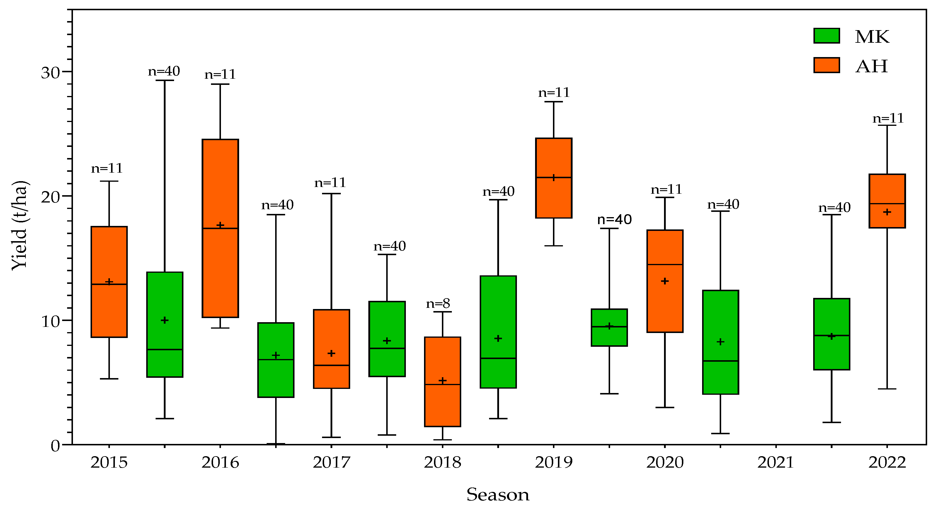
Historical mango yield data (2015–2022) from a total of 51 blocks were acquired from two growers (AH and MK farms) in the Northern Territory of Australia. The yield distribution is shown in Figure 2. To remove the influence of variation in tree numbers and land area or orchard size, the yield measured and reported in kilograms per block was converted to tons per hectare (t/ha) [50]. Farm data which were provided in different formats (e.g., TCEs or Kg) were harmonized into a uniform unit (t/ha). Furthermore, farms with mixed block yields were removed. Table 2 provides details of the two farms including cultivars grown (“Kensington Pride” (KP), “R2E2”, and “Calypso” (CAL)), tree age, and average yield. Yield data from six “independent test” farms (NTK1, NTK2, NTBS, NTM, NTKF, and QLDCF spanning the period 2015–2020) were used to validate the model calibrated using AH and MK farm data. This was done to assess the potential of the combined farms model to predict yield from those farms. Apart from the QLDCF farm, which is located in Queensland, all the other five “independent test” farms are located in the Northern Territory. A total of 350 data points was available for the analysis over the two study farms (Table 2). Additionally, a total of 34 data points was available for the farm level validation conducted on the six independent test farms.

2.2.2. Weather Data

Data on weather variables expected to influence mango orchard yield were extracted from the Australian Government’s SILO platform (https://www.longpaddock.qld.gov.au/silo) (accessed on 5 June 2023) which is a repository of climate data from 1889 to date, with a 5 km resolution. SILO was used because it provides daily datasets for a range of climate variables in suitable biophysical modeling formats. The six weather variables extracted for this study included monthly rainfall (Prec), minimum and maximum temperature (Tmin and Tmax), solar radiation (Rad), evapotranspiration (ETo), and vapor pressure deficit (VPD). Figure 3 shows the distribution of monthly total rainfall and average temperature in the study farms region over the eight-year time series.

2.2.3. Satellite Remote Sensing Data

This study used satellite imagery from the Landsat archive [51]. This global coverage dataset is free and has spatial and temporal resolution values of 30 m and 16 days, respectively, sufficient for the commercial mango orchards under investigation. Shapefile format boundaries of all the 51 blocks of the two farms were imported into the Google Earth Engine (GEE) platform [52] for the block-level spatio-temporal data extraction. Similarly, farm boundary shapefiles were used in the case of the six independent farms. The study used atmospherically corrected and cloud masked Landsat 7 ETM and 8 OLI (collection 2, tier 1—L2) data spanning the period from 2013 to 2022. Although Sentinel-2 (S2) which was launched in 2015 has better spatial (10–20 m) and temporal (5 days) resolution, Landsat data were used in this study because earlier data (prior to 2015 when S2 was launched) were needed for model development.
Following the image filtering step in GEE which filtered out all images with cloud cover >10%, the statistics of selected individual images were subsequently extracted to calculate different VIs (Table 3). Block and farm (in the case of the independent test farms) specific remote sensing data were extracted using Google Earth Engine (GEE) [52] and further analyzed with the R statistical software version 4.1.2 [53]. Therefore, four VIs derived from the surface reflectance values of the Landsat bands were used in this study (Table 3). Figure 4 shows the annual average GNDVI for the study farms (AH and MK) and the independent test farms over the time series.

2.3. Preparation of Input Variables for Yield Modeling

Different data aggregation methods were tested to select optimal variables with the greatest potential of predicting the pre-harvest yield of mango. The median values of the four VIs were calculated over different periods and the best option was selected. In the best aggregation option, three periods (3Ps) within a given growing season that begins from December of the previous year (when pruning may have been undertaken following harvest in the season) to November of the current year were used. Aggregates included P1, from December (of the previous year) to March of the current year (D–M); P2, April–July (A–J); and P3, August–November (A–N). This method of aggregation (3) proved to be ideal since P1 and P2 were found to be related with yield and came earlier than P3 which coincides with the fruit harvesting period. Subsequently, for each given year, P3 of the current year was removed from the dataset (as it was within the targeted three-month time window of commercial harvest (September ending or November), but previous years P3 were included as predictors in the subsequent models trialed (Table 4). Various periods obtained from the aggregation of respective months in a given growing season were matched to corresponding phenological stages observed in the study area (Figure 5).
A total of 32 remote sensing predictors were obtained from the four vegetation indices over 8 periods. A similar aggregation approach was conducted on the six weather variables to produce 48 predictors. A table describing all the 80 predictors is presented in Table S1. Subsequently, a correlation analysis was conducted to test the relationships among the response (yield) and the predictor variables (remote sensing VIs and weather). Additionally, yield prediction models were developed for the two farms separately and in combination and their performance assessed. To test the performance of the combined farms model to predict yield in individual farms (AH and MK), the models were trained with data from the two farms and validated on an independent test year of the individual farms. Furthermore, to test the ability of the combined farms model to predict yield beyond the scope of the calibration farms (AH and MK), the model was validated using data from the additional six independent test farm locations in NT and Queensland.

2.4. Yield Modeling Approaches and Techniques

2.4.1. Cumulative Training Year (CTY) and Leave-One-Year-Out (LOYO) Approaches

Two main data analysis approaches, i.e., CTY and LOYO, were tested in the R Statistical environment to determine the optimal method for predicting the test years at the block level and to assess the temporal variability of the models. For both approaches, the trained model was tested on only one year, which was not included in the model calibration. On the one hand, in the CTY approach, models were trained with only data from the year(s) prior to the test year [6]. Thus, for instance, to predict yield for 2017, data from 2015 to 2016 were used for model training and tested on 2017 independent data (Figure 5). On the other hand, in the case of the LOYO approach, data from every other year, apart from the test year, were used to train the model and the year that was left out in the training was used for model testing [6,59]. Thus, to predict 2019 yield under LOYO, the models were trained with data from 2015, 2016, 2017, 2018, 2020, 2021, and 2022. This approach makes available more data points for model training at the initial years compared to the CTY.

2.4.2. Hyperparameter Tuning

The “caret” package [60] was used to tune all six ML models including “XGBOOST” (xgbTree), “random forest” (rf), “SVR” (svmRadial), “PLSR” (pls), “RIDGE” and “LASSO” (glmnet) [61,62]. Other packages including “ggplot2” [63] were used to perform various functions in the model training, testing, accuracy assessment, and graphical display of results. Furthermore, to ensure the models were optimized and less susceptible to overfitting, a K-fold cross validation with 10 iterations was conducted in R to select the best tuning parameters during model training. Additionally, knowing that most of the variables used are highly correlated, tuning the regularization parameters in the respective models reduced deleterious effects of multicollinearity between predictor variables [40]. For instance, in both RIDGE and LASSO regression modeling, a critical consideration is the selection of lambda (λ), which represents the penalty term [22]. Table 5 shows the ML algorithms trialed in the current study with their respective relevant hyperparameters. The specific best tune parameters for the six algorithms are presented in Table S2.
The shrinkage methods such as PLSR, RIDGE, and LASSO, otherwise known as regularized linear regression algorithms, trialed in this study, not only fit ML models but apply weights to model coefficients in order to reduce the impact of less important predictors.
The nonlinear algorithms (XGBOOST, SVR, and RF) were chosen for this study because of their proven efficiency in various ML studies on crop yield prediction as well as their ability to learn complex relationships in data [23,40].

2.4.3. Bootstrap Sampling of Training Dataset

Due to the limited number of data points available for this study, bootstrap sampling was conducted on the training dataset in order to provide a measure of the variability of the prediction accuracy [67]. Bootstrapping is a statistical technique that simulates the replication of a sample from a population by resampling [67,68,69]. Bootstrapping is effective for estimating the distribution of model prediction errors [68]. In this study, the training dataset for each year was resampled randomly with replacement for varying numbers of sample size (n) including n = 50, 100, 150, etc., and iterated 100 times. The result was presented in a boxplot to show the effect of an increased number of training samples on yield prediction errors.

2.4.4. Model Prediction and Performance Evaluation

Mango yields at both the block level and the farm level were predicted from the six ML algorithms trialed and their performance assessed. Production (tons (t)) at the block level and farm level was computed using:
P t   =   Y × A
where P is the production, Y is the yield, and A is the area of the block/farm.
The predicted yield was plotted alongside the actual yield measured by the growers to visually compare the accuracy of the predictions. The null model [70] was used to establish the prediction accuracy assessment baseline to also compare complex models. This model predicts the test year yield based on the average of the yield in the training years.
The evaluation metrics used in this study were mean absolute error (MAE), normalized mean absolute error (NMAE), and farm level error of model (FLEM). MAE is less sensitive to outliers than RMSE [71,72]. In order to validate the performance of the model at the block level, we calculated MAE (Equation (2)) as:
MAE t / ha   =   1 N × i = 1 N y ¯ i y i
NMAE was used because it is a straightforward metric that is easy to interpret and to compare results with other studies, where the mean yield for different crops is very different [22,73]. The MAE was divided by the mean of grower observed yield, Y ¯ , and expressed as a percentage as shown in Equation (3).
NMAE %   =   MAE Y ¯ × 100
The accuracy was calculated as 100 − NMAE (%).
Similarly, block-level predictions (production in tons using Equation (1)) for each farm were summed and compared with the respective block-level yield data obtained from growers per year. This was converted to percentage error of the model (FLEM) by finding the absolute difference of the sum of block-level predictions (Pred) and the sum of the block-level actual yield (Act) divided by the sum of block-level actual yield expressed as a percentage (Equation (4)):
FLEM %   =   abs Pred     Act   Act × 100
The farm-level accuracy of the model was calculated as 100 − FLEM (%).

3. Results

In Section 3.1, we present the findings on the assessment of relationships among yield and the RS/weather (WV) variables by exploring which predictors best explain the variability in the actual yield. The results from predictive forecast models built using (i) only RS variables and (ii) a combination of RS and WV, and predictions assessed at the block- level and farm-level are presented in Section 3.2 and Section 3.3, respectively. Findings for predicting individual farm yield from the combined farms model and validating the same on independent test farm locations are presented in Section 3.4 and Section 3.5, respectively. Finally, in Section 3.6, we report the findings for the assessment conducted on the impact of training data size on the study.

3.1. Relationships among Yield and the Predictor (RS and Weather) Variables

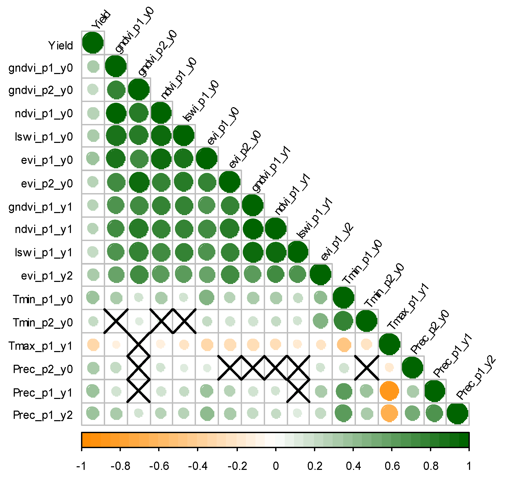
To determine the relationships among yield and the predictor variables (RS and weather), a correlation analysis was conducted. Figure 6 shows the correlations among yield and the 16 best RS/weather predictors among the 80 predictor variables studied, based on significance. Generally, precipitation was positively correlated with yield, while Tmax was negatively correlated with yield. All VIs were positively correlated with each other and with mango yield. Specifically, the enhanced vegetation index (EVI) in the first period of the prediction year (evi_p1_y0) was the best RS predictor with a correlation coefficient (r) of 0.38, followed by the green normalized difference vegetation index (GNDVI) in the first period of the prediction year (gndvi_p1_y0). Rainfall in the first period of the second year prior to the prediction year (Prec_p1_y2) was the best weather predictor with r = 0.4, followed by the minimum temperature in the first period of the prediction year (Tmin_p1_y0) with r = 0.39.

3.2. Predicting Mango Yield at the Block Level and the Farm Level Using RS Variables Only

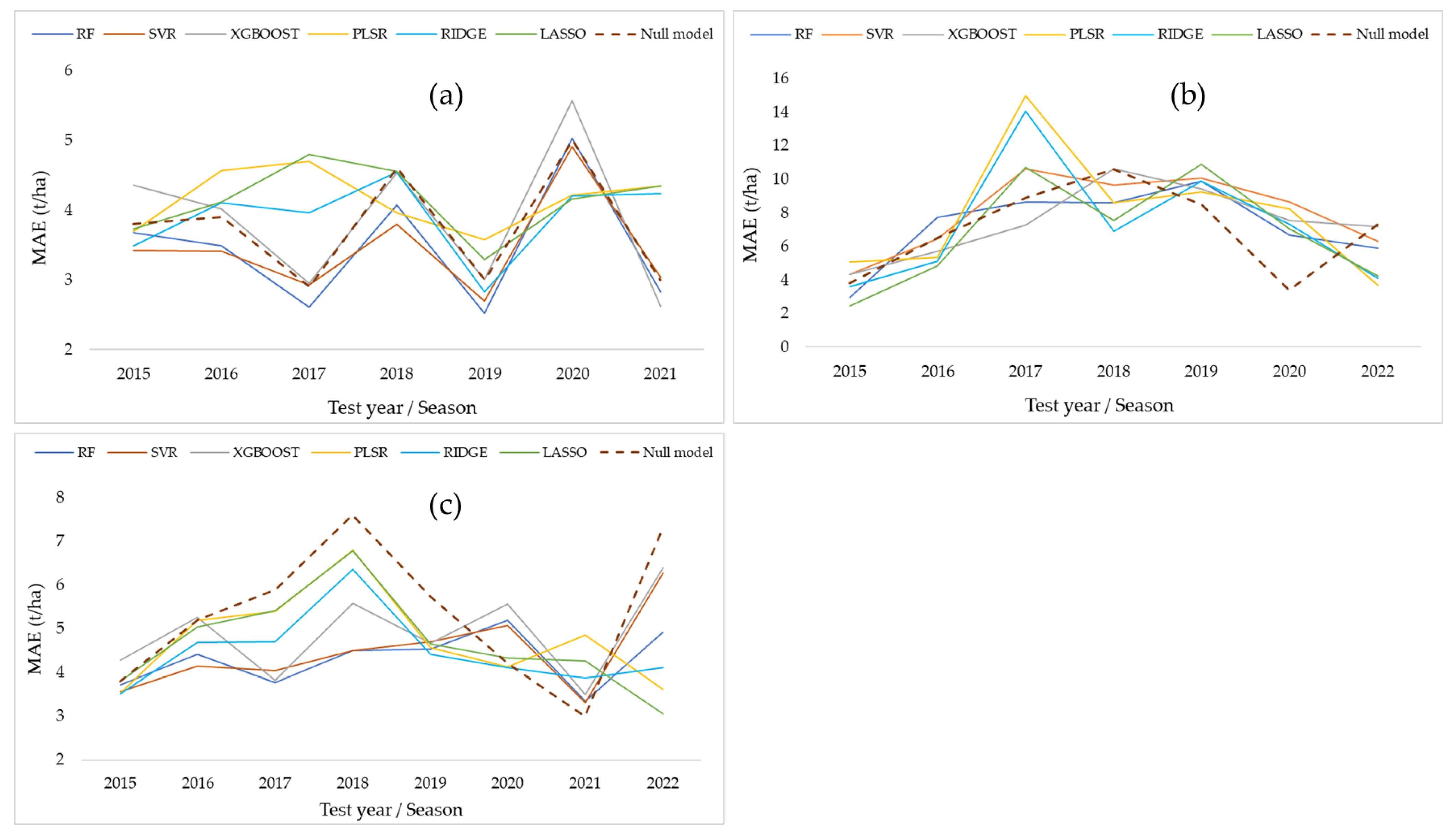
The models were trained using only RS variables, with data both from the MK farm and the AH farm, and the LOYO training/testing strategy was applied. Generally, the RF model using this strategy provided the best predictions (average MAE = 4.3 t/ha), and XGBOOST provided the worst predictions (average MAE = 4.9 t/ha). As shown in Figure 7, some years were predicted more accurately than others, with 2015 the best (average MAE = 3.7 t/ha) and 2018 the worst (average MAE = 5.8 t/ha). The remote sensing models provided lower errors on average than the null model, demonstrating the utility of the modeling approach.
Using RS variables only for the MK farm, the 2019 RF model was the best prediction year with an MAE (RMSE) of 2.5 (3.3) t/ha at the block level. The 2020 XGBOOST model performed the worst with an MAE (RMSE) of 5.6 (6.5) t/ha (Figure 7a). The 2015 LASSO model performed best for the AH farm with an MAE (RMSE) of 2.4 (3.6) t/ha. Furthermore, for the AH farm, the 2017 PLSR model (Figure 7b) was the worst performing with an MAE (RMSE) of 15.0 (16.3) t/ha. For the combined farms model (Figure 7c), the 2022 LASSO model was the best with an MAE (RMSE) of 3.1 (3.8) t/ha which was closely followed by the SVR and RF models of 2021, with MAE (RMSE) values of 3.3 (4.0) and 3.4 (4.0), respectively. LASSO and PLSR of 2018 performed worst with MAE (RMSE) values of 6.8 (7.6) and 6.8 (7.4) t/ha, respectively.
The yield prediction error at the farm level (using the FLEM metric from Equation (4)) was generally lower than that ay the block level for both the AH farm and the MK farm as well as the combined farms model. Table 6 shows the results of the combined farms model. The lowest farm-level error (4.3%) was recorded in 2015 and 2021, and the highest farm-level error (38.6%) was observed in 2017.
The Supplementary Material (Figure S1) shows the scatter plots of the best and worst models for the AH farm and the MK farm as well as the combined farms model using RS variables only. Furthermore, variable importance plots from the RS-based RF model for the combined farms model for 2015, 2019, and 2021 test years are shown in the Supplementary Material (Figure S2).
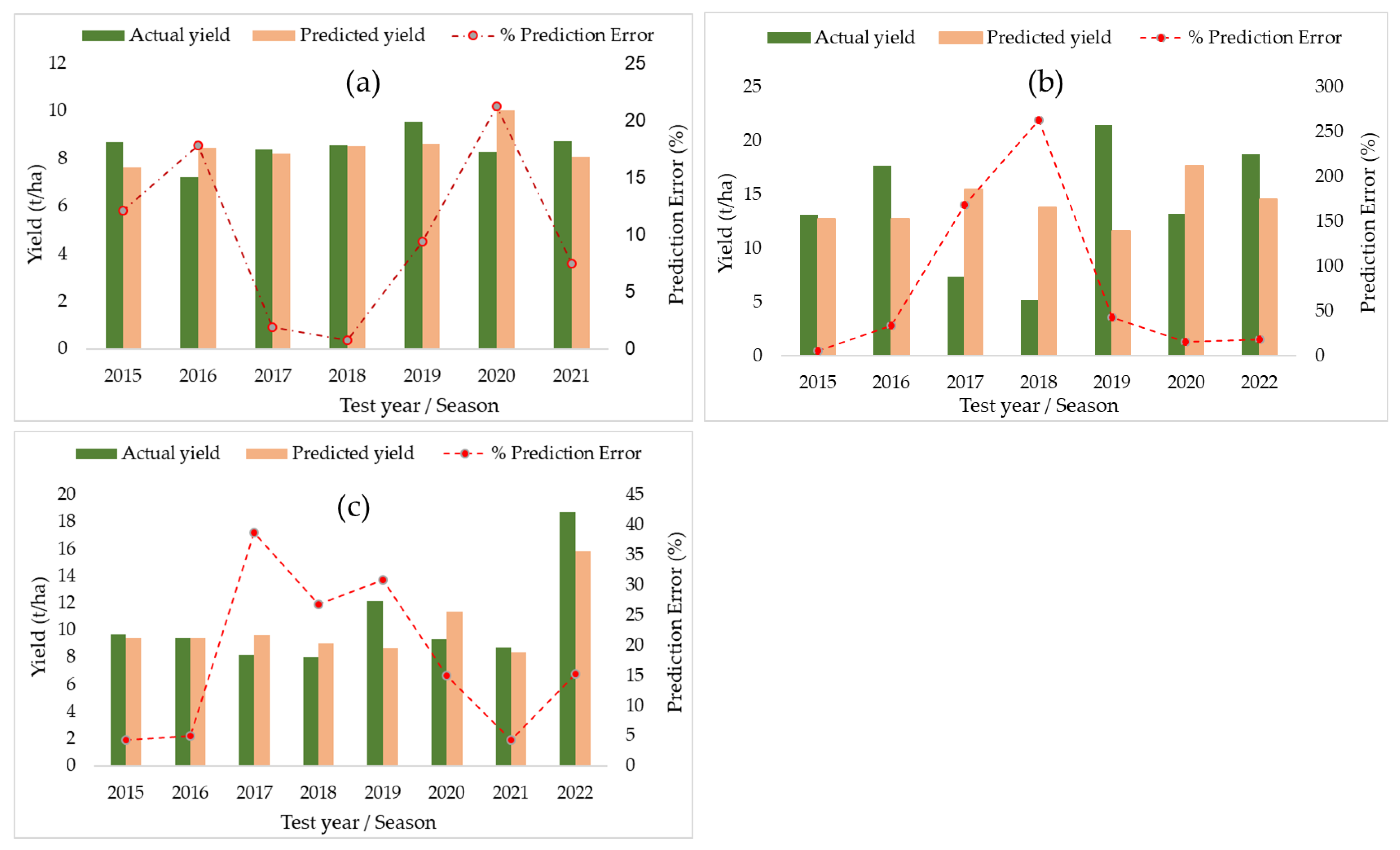
Figure 8 shows the average farm-level yield predicted for each year (from 2015 to 2022) for the AH farm, the MK farm, as well as the combined farms model, using the RS-based RF model. The farm-level error (FLEM) of the RS-based RF model ranged from 0.8% to 21.2% for the MK farm, and for the AH farm, it ranged from 5.3% to 43.2%. The farm-level error for the best combined model was 4.3% (accuracy of 95.7%) which was recorded for the 2021 season.

3.3. Predicting Mango Yield at the Block Level and Farm Level Using RS and Weather Variables

The potential of weather variables to improve the performance of RS-based yield prediction models was explored by integrating six weather variables and four RS-based VIs in a combined predictive model. For the MK farm (Figure 9a), the nonlinear models performed consistently better than the linear models.
Previously, the performance of the model developed using only RS variables was explored. This section looks at the general performance of the models trained with RS and WV variables with data both from the AH farm and the MK farm. Again, the LOYO training/testing strategy was adopted. Generally, the RF model produced the best predictions (average MAE = 4.8 t/ha), and LASSO the worst (average MAE = 8.3 t/ha) across the time series. The models produced predictions with varying accuracies, i.e., high in some years and low in others. The 2015 test year was the best with an average MAE of 4.3 t/ha and the 2022 test year was the worst (average MAE = 7.6 t/ha).
Figure 9 shows the performance of the six ML algorithms trialed in this study. Mango yield prediction error at the block level was generally higher than that at the farm level for both the AH farm and the MK farm as well as the combined farms model using both RS and weather variables. For example, the FLEM for the farm level ranged from 3.7% to 82.7% compared to from 28.7% to 70.7% at the block level using the RF algorithm on the combined farms model (Table 7). The farm-level error was larger than the block-level error particularly in the test year 2017 due to extremely low actual yields observed in six blocks of the AH farm. This produced very large production errors of the prediction at the farm level.
The best prediction year for the combined farms model was the 2021 RF model, which outperformed all the other algorithms, with an MAE (RMSE) of 2.9 (3.5) t/ha. The worst performance of the combined farms model was observed in the 2021 LASSO model with an MAE (RMSE) of 15.1 (15.8) t/ha. It is useful to produce a universal model that is able to predict yield irrespective of year, cultivar, and farm location with acceptable error.
The Supplementary Material (Figure S3) shows the scatter plots of the best and worst models for the AH and MK farms as well as the combined farms model using RS and weather variables.
The summaries of results presented in Section 3.2 (RS only) and Section 3.3 (RS + WV) suggest that adding weather variables only marginally improved the results by 0.5 t/ha as compared to RS only, which is not considered substantial. Therefore, the subsequent predictions are done using RS variables only with RF algorithm, the results of which are presented in the following sections.

3.4. Predicting Individual Farm Yield from the RS-Based Variables

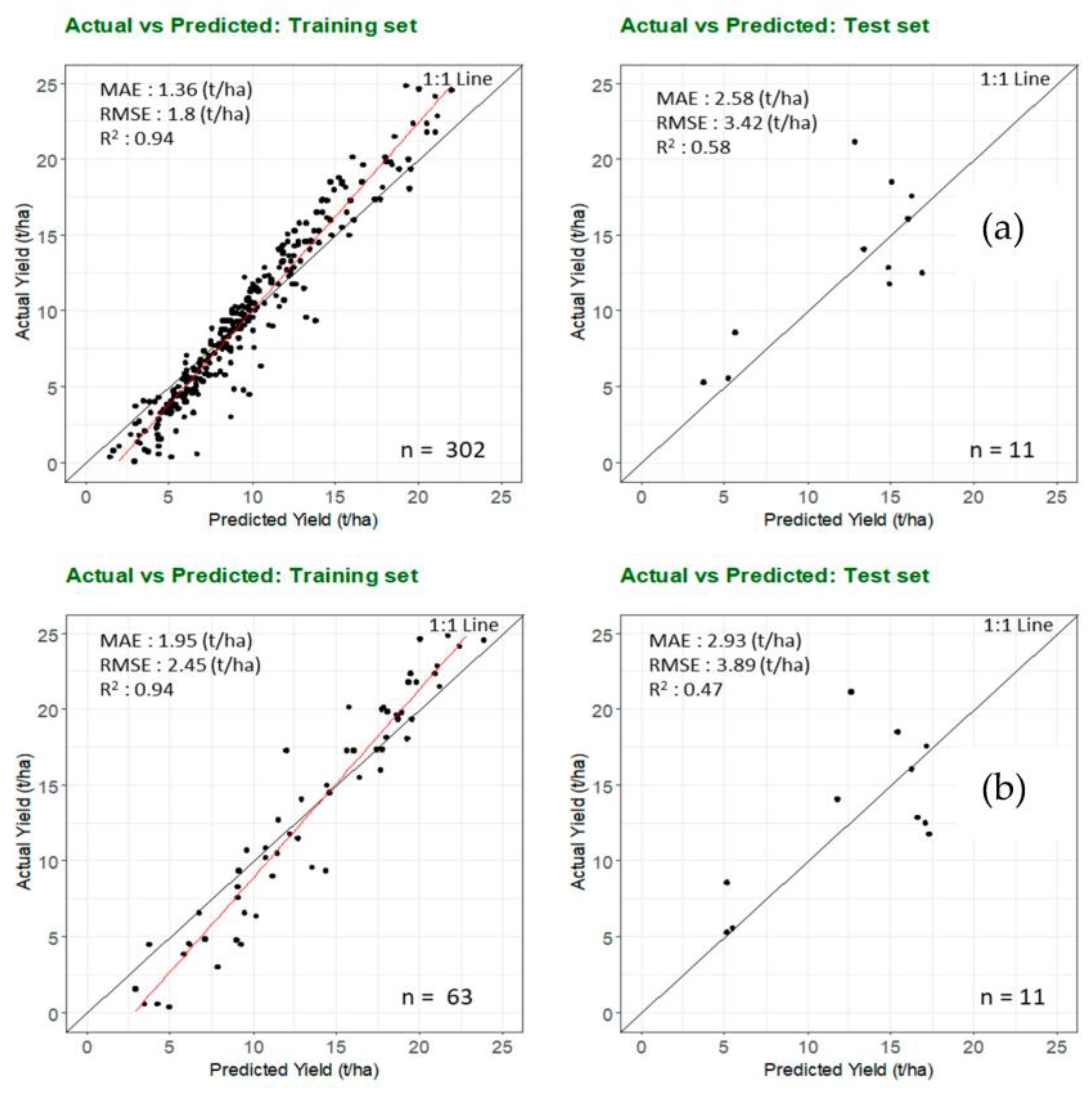
In the previous sections, we reported models trained using data from both farms. In the current section, we compare that method to models trained and tested on single farms. This could be due to the possibility of one farm contributing more to the model accuracy. To determine this, two different assessments were conducted as follows: (a) evaluating a model trained using both farms’ data (combined model) and testing on an individual farm and (b) evaluating a model trained and tested on the same farm. The assessments both used RF models based on the LOYO approach. The RF model trained with data (2016–2022) from the two farms (AH and MK) and tested on an independent year (2015) of an individual farm (AH) (Figure 10a), produced accuracies marginally better (MAE = 2.6 t/ha, R2 = 0.58) than the one trained and tested on an individual farm data over the same period (MAE = 2.9 t/ha, R2 = 0.47) (Figure 10b). The farm-level prediction error for both models (FLEM) was <10%.
Although this result varies from year to year, the average across all years for the AH farm was consistent with the 2015 observation. The opposite happened in the case of the MK farm for the 2015 test year. However, the result was comparable on average (MAE for MK, MK = 3.5 t/ha and combined farms, MK = 3.6 t/ha) across the time series for the MK farm.

3.5. Validating the Combined Model on Independent Test Farm Locations—RS Variables Only

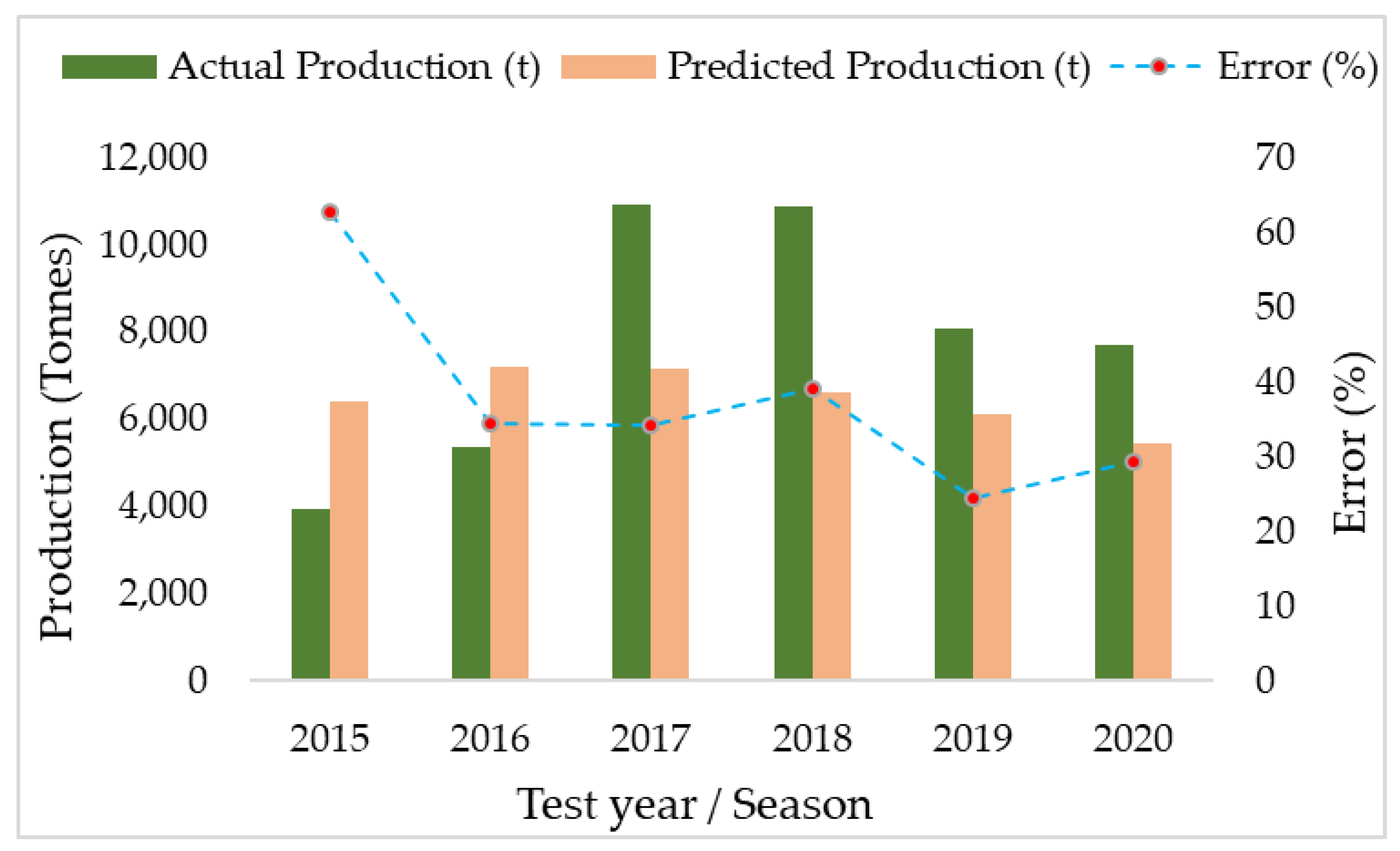
The potential of the combined model developed from the AH farm and the MK farm to predict yield from farms not used in the calibration of the model (independent test farms) was also assessed. For 2016–2020, the RF model produced errors ranging between 24% and 39%, whilst for the 2015 season the prediction error was above 50%. The model generally overpredicted in the first two years and underpredicted the rest of the years, with 2017 and 2018 being the highest overprediction years. Figure 11 shows the actual and predicted production for the six-year time series.
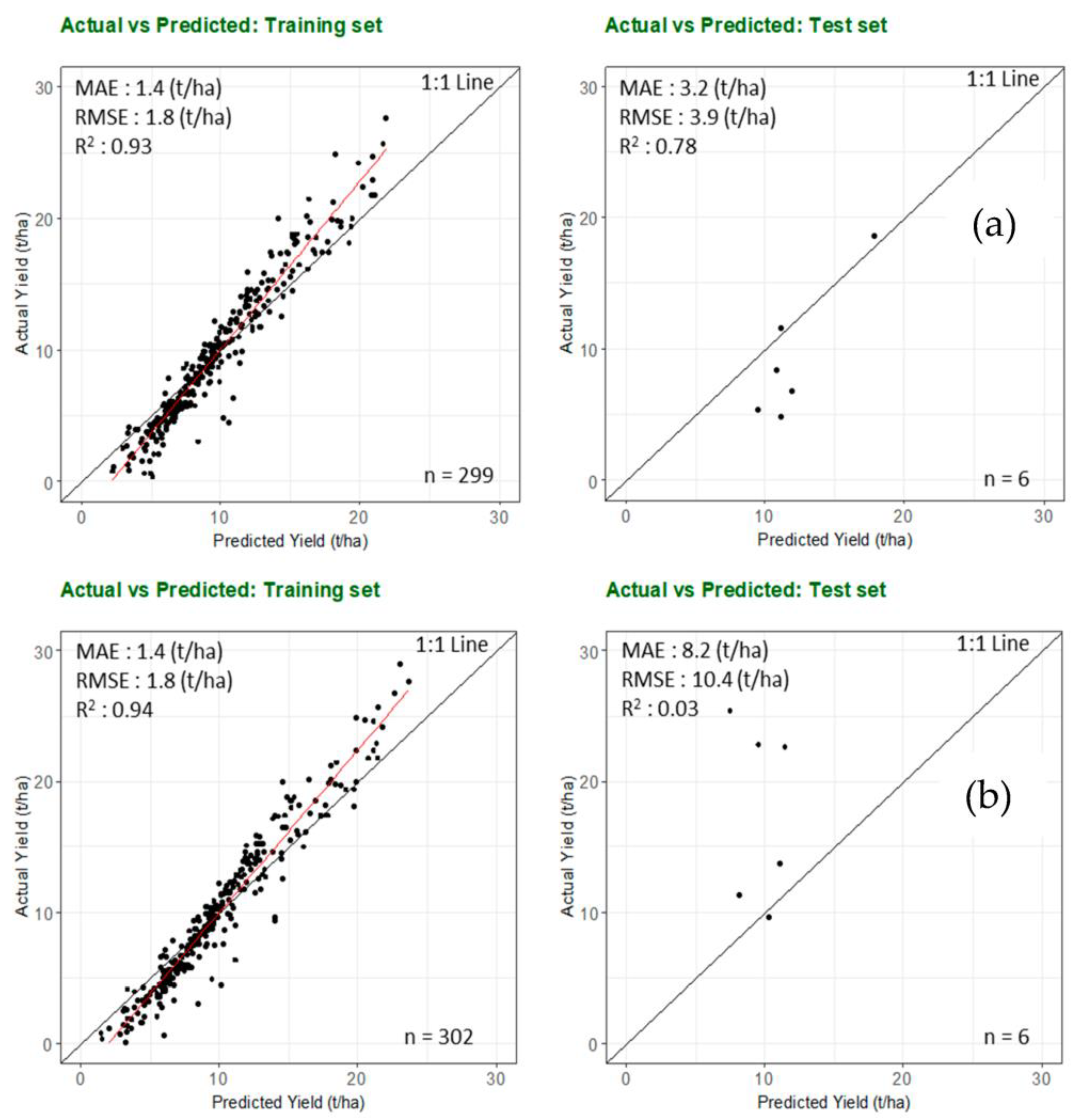
The best (RF 2016) and worst (RF 2018) performing models for the independent test farms validation exercise are shown in Figure 12. The MAE (RMSE) for the best performing model was 3.2 (3.9) t/ha.

3.6. Impact of Training Dataset Size

Figure 13 shows the results of the bootstrap sampling exercise conducted on the combined AH and MK farms training data for 2016–2022, to predict the 2015 yield using the RS-based RF model. This shows expectation of prediction accuracy with random permutations in the training dataset, and with different number of training data points. Increasing the number of sampling points reduced uncertainty and errors in the predictions. With 50 points the median MAE was 4.0 t/ha (standard deviation was 0.29), and with 250 it was 3.7 t/ha (standard deviation was 0.05).

4. Discussion

4.1. Predictor and Response Variables Relationship in Yield Modeling

Although correlations achieved among the response (yield) and predictor (RS and WV) variables were quite low as indicated by the correlation coefficients of the best predictors (r < 0.5, Figure 6), they were, however, significant at p < 0.05 and allowed for the development of the predictive models in this study. The EVI and the GNDVI were found to be the best RS predictors of mango yield. These indices have characteristics (high chlorophyll sensitivity with wider dynamic range [56]) that make them superior to the widely known and used NDVI for this application. As observed by Rahman and Robson [74] and Brinkhoff and Robson [22], in a separate study on sugarcane and macadamia, respectively, the GNDVI was found to be the best predictor of yield. The EVI, however, in a study that assessed the potential of Sentinel-2 RS data to retrieve mango phenology, was found to be the best related index among the four (including NDVI, GNDVI, and SAVI) trailed [14]. The EVI is an optimized VI that corrects for atmospheric conditions and canopy background noise and has high sensitivity in high biomass areas such as mango tree canopy [14,75,76].
The rainfall in the first period of the second year prior to the prediction year (Prec_p1_y2) and the minimum temperature in the first period of the prediction year (Tmin_p1_y0) were found to be the best weather predictors. Interestingly, although their correlation coefficients were slightly higher than that of the RS predictors, our study found that weather variables did not significantly improve the performance of the models developed, rather they were largely comparable with the results from RS variables only. The observation aligns well with other studies [22,70,77] that support the use of only RS variables in building such models, as RS variables have the capacity of capturing the effects of weather on crop biophysical properties and other parameters such as yield. This finding could largely be due to the coarse resolution of the weather data in this study which could not describe the spatial variability across the mango orchard blocks. It has to be noted, however, that this does not rule out the importance of weather variables in such studies especially if critical temperatures are breached during key growth stages [78]. Thus, a conscious effort must be made to obtain weather data of finer resolution that enables the efficient modeling of spatial variability. It is envisaged that with a larger dataset with more years and more locations, more variability in weather would be observed, and thus the relationship between weather and yield may be more obvious.
Apart from rainfall, all the highly correlated RS and weather variables coincided with Periods 1 and 2 (p1 and p2) of the prediction year which span the period December of the previous year to July of the current year. This period ends approximately 3–5 months prior to the commencement of the harvest season in September/November. In terms of phenology aggregation, p1 and p2 coincide with the flushing and flowering/fruitset, respectively, fruit development stages. Thus, yield can be predicted at least 3 months before the harvesting season.

4.2. Block Level and Farm Level Yield Prediction

Model performance at the block level showed errors (NMAE) ranging between 31.2% and 52.5% by season and algorithm tested. At the farm level, the RS-based RF model prediction errors ranged from 0.8% to 21.2% for the MK farm and from 5.3% to 43.2% for the AH farm. Thus, the errors were reduced for both the RS only and RS + WV models at the farm level (Table 6 and Table 7). The finding agrees with that of Brinkhoff and Robson [22], Filippi et al. [79], and Deines et al. [70] that the application of yield prediction models developed at finer resolution (e.g., block level) to predict yield at a coarser scale (e.g., farm level) tends to reduce errors, as positive (overprediction) and negative (underprediction) errors tend to cancel each other out. Although Sinha and Robson [26] and Rahman et al. [9] used very high resolution World View-3 satellite data and a different yield prediction approach where an infield in-season mango fruit count for 18 individual trees of different vigor (high, medium, and low) were used for model calibration (details can be found in [9]), and their results were found to be consistent with the results obtained using a time series approach in this study (RS only (error of 4.3% = accuracy of 95.7%) and RS + WV (error of 3.7% = 96.3% accuracy). Unlike annuals, yield prediction of perennial tree crops such as mango is very challenging. The range of accuracies obtained in different seasons could be due to different factors such as weather, management, biennial bearing, nutrient use/carbohydrate storage, etc. Most of these factors were not included in our model because they were beyond the scope of this initial study. However, inclusion of these factors in a subsequent study has been proposed to determine their influence on model accuracy. Previous studies for tree crop yield prediction reports on relative accuracy measures for direct comparison are hard to find [80]. We compared our results to other fruit crops and found that the accuracy of our best models aligns well with the results of the existing studies outlined in Table 1 ranging from 73.6% to >90% (e.g., for Apple (>90%), Citrus (96%), and Grape (85.95%). The novelty of our approach is in its ability to use freely available satellite imagery spanning a period of 8 years (2015–2022) and training models on out-of-season commercial yield data. Additionally, unlike the earlier methods (Table 1) which are largely in-season infield approaches, our research presents a method that is less expensive, less laborious, and can produce predictions at least 3 months before the harvest period.

4.3. Comparison of Model Performance

Generally, there is no universally accepted best or worst performing model and hyperparameter set in the field of modeling and ML [81,82]. According to Goodfellow et al. [81], the performance of a given model compared to another is determined by the type, number, and nature or complexity of the dataset that is fed to it or being manipulated. For instance, there could be a situation where a simple or multiple linear regression based on the ordinary least squares (OLS) method could fit data better than a complex ML method such as XGBOOST. Therefore, the discussion in this section is not to declare a particular algorithm as best or worst in all cases globally, but rather emphasize their performance in relation to the particular data under investigation. In this study, the nonlinear models outperformed all the regularized linear models. This could be largely due to the complexities and variability in mango yield from year to year which is captured better by the nonlinear algorithms [15,39]. However, this observation is inconsistent with the finding by [22], who reported that a RIDGE regularized regression model outperformed nonlinear ML models tested such as SVR and RF.
The study noted the consistency of the RF model’s performance and its high level of adoption in this field. Furthermore, the variable importance (varImp) function made it easier to identify the variables that contributed more to the predictions. For example, the varImp plot for the RS-based RF models for 2015, 2019, and 2021 (Supplementary material, Figure S2) showed the top five variables that contributed to the model in the respective years. Consistently, evi_p1_y0, evi_p1_y1, gndvi_p3_y1, gndvi_p1_y0, and lswi_p2_y0 were among the top five. The results of this study further showed that the best predictor variables differed from model to model and site to site which reinforced the observation of Fukuda et al. [39], who used RF to predict mango yield under various irrigation schemes during the dry season in Thailand. Finally, no single algorithm trialed outperformed all others across all test years and farms. This, therefore, supports the argument that no single algorithm or model is universally adjudged the best or worst in all circumstances [39,81]. However, practically, when an analyst is asked to deliver the forecast for the next year, for example, there will be a need to choose one, or provide predictions from multiple ”good” models. The ”best’’ model for next year cannot be picked since the actual yield data are unavailable when the forecast is provided.

4.4. Potential for Yield Prediction on Independent Farms

The developed models were tested on independent farms not used in model calibration and it was found that the errors were, on average, between 24% and 39% across the time series, except the 2015 test year with an error >50% (Figure 11). Thus, the model has the potential to predict mango yields in independent test locations without the need for yield data from those locations for model calibration. Although the combined model was developed from only two farms (AH and MK) with three cultivars (Kensington Pride, R2E2, and Calypso), the results from the extrapolation of this model to other independent test farms does indicate some potential to predict yield with satisfactory accuracy at farms where data are unavailable. Due to data unavailability stemming from the difficulty of obtaining block-/farm-level data from growers, it was challenging to validate this finding beyond two regions. Yield data for one farm from a different region (Queensland), apart from the NT where the models were originally calibrated, were used and the results indicated an accuracy ranging between 61% and 76% from 2016 to 2020. This is an important outcome considering the difficulty in obtaining accurate farm-level yield data for the calibration and validation of yield prediction models. With the availability of more farm-/block-level data in the future, the ability of a single model to predict yield across independent test farms/regions and cultivars could be explored and improved. This is a capability that is reinforced by the findings of Khaki et al. [83] who used convolutional neural networks (CNNs) and recurrent neural networks (RNN) to successfully generalize the yield of maize in independent test locations.

4.5. Bootstrap Results—Varying Training Sample Size

The results from this study lay credence to the fact that more or an adequate number of training data points is required for model stability and accuracy improvement [59]. In the current study, it was observed that fewer data points produced estimates with larger variation from the mean, i.e., high model uncertainty. With the availability of more data, the variation reduced, producing a more stable estimate of the error associated with the prediction (Figure 13). For example, with 50 training points, the average MAE was 4.0 t/ha, while with 250 training points it was reduced to 3.7 t/ha. This observation agrees with the position of Brinkhoff et al. [84] that ML models for yield prediction trained on more data produce more accurate results than those trained on fewer data points. van Klompenburg et al. [80], in a systematic review of crop yield prediction using ML models, noted that the major limitation of such studies reported by researchers was data insufficiency challenges.

4.6. Challenges with Input Data Quality and Cleaning

The robustness of any given model is largely a function of the quality of the input data used in its training and testing. Although some algorithms may outperform others, irrespective of the type used in model development, good quality data will result in a better performing model than bad quality data. This agrees with the thoughts of Teich [85] and McDonald [86] who reiterated the need to pay attention to data quality in any machine learning model calibration and validation campaign. Therefore, it is imperative for any model building and testing process to critically consider the cleaning of the input data, since it holds the key to the performance of the final model [59]. For ML models, it is imperative to have an adequate number of quality observations or data points for the algorithm to learn the problem to be solved [59]. In situations where data are not clean, what the model learns eventually is the noise in the data which results in unstable models. Generally, the errors associated with models developed in this study, especially at the block level, could be due to uncertainties in grower supplied data. This involves the limitations associated with the amount of input data available for model building and probably variations in the accuracy and efficiency in data collection protocols across blocks and orchards. According to growers, factors such as weather, labor shortage, irregular yield patterns, and lack of equipment contribute to their inconsistency in data collection protocols. In some cases, for example, some growers combined data from different blocks and reported them as one block due to the reasons mentioned earlier. This results in a situation of a myriad of inconsistencies that require extensive data cleaning to harmonize and make usable. NMAE at the block level (33.6%), in the current study, was higher than that observed by Brinkhoff and Robson [22] in a macadamia study (20.9%) in Australia owing to the challenges discussed above.
Additionally, planting different cultivars in one farm can negatively influence model performance due to factors such as age of the planted cultivars, growth dynamics, and yield variability per cultivar [6,22]. In spite of the uncertainties associated with the modeling process, this study produced a range of prediction errors at the farm level from year to year that is well within the limit consistent with Anderson et al. [10], who reported the acceptable targets (10–20%) by fruit tree producers supplying multiple and easily accessible domestic markets. It is, therefore, expected that model performance will improve significantly as data collection protocols are standardized across blocks/orchards in growing areas and more high-quality data are made available.

5. Conclusions

Pre-harvest yield prediction is critical for planning harvesting and marketing logistics as well as farm profitability management, resulting in a reduction in wastage in the mango value chain. This study has demonstrated the capability of different ML algorithms to predict mango yield at least 3 months ahead of the harvesting period from VIs derived from time series Landsat satellite RS data. It was concluded that applying the random forest algorithm with only remote sensing variables produced results that were comparable with models that combined both RS and weather variables. Therefore, it is recommended that for such studies, if no block-specific weather data are available, one could focus on only remote sensing variables to predict block-level yield. The prediction of farm-level yield was far more accurate than that at the block level, which was likely the result of under- and overpredicted blocks cancelling each other out. Additionally, training models with data from multiple farms produced better predictions than models trained using data from individual farms. This study highlighted the difficulties in acquiring accurate farm-level data for the calibration and validation of models and the need to undertake a proper cleaning and harmonization of model input data to guarantee accurate predictions. In spite of these challenges, this study presents a method that makes a promising initial contribution to the use of time series data in the development of pre-harvest mango yield prediction models at multiple scales (block and farm). This study demonstrated the ability to generalize and generate better estimates at a coarser scale than simply using previous average yields. It is believed that, in the future, when more standardized block- and farm-level yield data are made available, this method could be repeated to predict yield for other regions and the nation as a whole. Finally, future research could explore the potential of this method to produce robust estimates in other countries and other perennial tree crops.

Supplementary Materials

The following supporting information can be downloaded at: https://www.mdpi.com/article/10.3390/rs15123075/s1, Figure S1: Best performing models (a–c) obtained from only RS variables at the block level for the farms (a) MK—RF 2019, (b) AH—LASSO 2015, and (c) combined farms—LASSO 2022, and the worst performing models (d) MK—XGBOOST 2020, (e) AH—PLSR 2017, and (f) combined farms—LASSO 2018, Figure S2: Variable importance plots for the RS-based RF model from the combined farms model for 2015, 2019, and 2021 test years. The red dashed bounding box highlights the top five predictors in each test year, Figure S3: Best performing models (a–c) obtained from the combined RS and Weather variables at the block level for the (a) MK—RIDGE 2019, (b) AH—RF 2019, and (c) combined farms—RF 2021, and the worst performing models (d) MK—LASSO 2017, (e) AH—LASSO 2015, and (f) combined farms—LASSO 2021, Table S1: Remote Sensing (RS) and Weather predictor variables (WV) used in this study, Table S2: Best tuned hyperparameter values for the six algorithms used for the combined farms (AH+MK) model in this study.

Author Contributions

Conceptualization, B.A.T. and M.M.R.; methodology, B.A.T., M.M.R. and J.B.; writing—original draft preparation, B.A.T.; writing—review and editing, B.A.T., M.M.R., J.B., A.R. and P.S.; supervision, M.M.R., J.B., A.R. and P.S.; funding acquisition, A.R. All authors have read and agreed to the published version of the manuscript.

Funding

This study has been funded by the Australian Government Department of Agriculture and Water Resources as part of its Rural R&D for Profit program and Horticulture Innovation Australia Ltd., grant number ST15002 (Multi-scale Monitoring Tools for Managing Australian Tree Crops) as well as with support from a Remote Sensing scholarship granted by the Applied Agricultural Remote Sensing Centre (AARSC) of the University of New England, Australia.

Data Availability Statement

The remote sensing and weather data are publicly available and those used in this study can be obtained from the corresponding author on request. The yield data are not publicly available due to commercial restrictions and privacy but could be obtained with a reasonable request from the growers.

Acknowledgments

The support of Abel Chemura, Edward Boamah, Ponraj Arumugam, Casey Naughton, and Richard Crabbe as well as managers and staff of all the study farms is highly acknowledged, for the invaluable contribution towards the success of this study. We also acknowledge the support from the Australian Government through the Destination Australia Program (DAP) Scholarship initiative.

Conflicts of Interest

The authors declare no conflict of interest.

References

  1. FAOSTAT. Value of Agricultural Production. Available online: https://www.fao.org/faostat/en/#data/QV (accessed on 8 January 2023).
  2. Mitra, S.K. Mango Production in the World—Present Situation and Future Prospect. Int. Soc. Hortic. Sci. 2016, 1111, 287–296. [Google Scholar] [CrossRef]
  3. Thompson, J.; Morgan, T. Northern Territory’s Lucrative Mango Industry 1000 Workers Short as Fruit-Picking Season Begins. ABC News. Available online: https://www.msn.com/en-au/news/australia/northern-territorys-lucrative-mango-industry-1000-workers-short-as-fruit-picking-season-begins/ar-AA11vvcI (accessed on 3 December 2022).
  4. NTFA. NT Mangoes. Northern Territory Farmers Association. Available online: https://ntfarmers.org.au/commodities/mangoes/ (accessed on 3 December 2022).
  5. DTF. Northern Territory Economy: Agriculture, Forestry and Fishing. Northern Territory Government. Available online: https://nteconomy.nt.gov.au/industry-analysis/agriculture,-foresty-and-fishing#horticulture (accessed on 3 December 2022).
  6. Zhang, Z.; Jin, Y.; Chen, B.; Brown, P. California Almond Yield Prediction at the Orchard Level With a Machine Learning Approach. Front. Plant. Sci. 2019, 10, 809. [Google Scholar] [CrossRef] [Green Version]
  7. Zarate-Valdez, J.L.; Muhammad, S.; Saa, S.; Lampinen, B.D.; Brown, P.H. Light interception, leaf nitrogen and yield prediction in almonds: A case study. Eur. J. Agron. 2015, 66, 1–7. [Google Scholar] [CrossRef]
  8. Hoffman, L.A.; Etienne, X.L.; Irwin, S.H.; Colino, E.V.; Toasa, J.I. Forecast performance of WASDE price projections for U.S. corn. Agric. Econ. 2015, 46, 157–171. [Google Scholar] [CrossRef]
  9. Rahman, M.M.; Robson, A.; Bristow, M. Exploring the Potential of High Resolution WorldView-3 Imagery for Estimating Yield of Mango. Remote Sens. 2018, 10, 1866. [Google Scholar] [CrossRef] [Green Version]
  10. Anderson, N.T.; Walsh, K.B.; Wulfsohn, D. Technologies for Forecasting Tree Fruit Load and Harvest Timing—From Ground, Sky and Time. Agronomy 2021, 11, 1409. [Google Scholar] [CrossRef]
  11. Anderson, N.T.; Underwood, J.P.; Rahman, M.M.; Robson, A.; Walsh, K.B. Estimation of fruit load in mango orchards: Tree sampling considerations and use of machine vision and satellite imagery. Precis. Agric. 2018, 20, 823–839. [Google Scholar] [CrossRef]
  12. Payne, A.B.; Walsh, K.B.; Subedi, P.P.; Jarvis, D. Estimation of mango crop yield using image analysis—Segmentation method. Comput. Electron. Agric. 2013, 91, 57–64. [Google Scholar] [CrossRef]
  13. Rahman, M.M.; Robson, A.; Brinkhoff, J. Potential of Time-Series Sentinel 2 Data for Monitoring Avocado Crop Phenology. Remote Sens. 2022, 14, 5942. [Google Scholar] [CrossRef]
  14. Torgbor, B.A.; Rahman, M.M.; Robson, A.; Brinkhoff, J.; Khan, A. Assessing the Potential of Sentinel-2 Derived Vegetation Indices to Retrieve Phenological Stages of Mango in Ghana. Horticulturae 2022, 8, 11. [Google Scholar] [CrossRef]
  15. Matese, A.; Di Gennaro, S.F. Beyond the traditional NDVI index as a key factor to mainstream the use of UAV in precision viticulture. Sci. Rep. 2021, 11, 2721. [Google Scholar] [CrossRef]
  16. Verma, H.C.; Ahmed, T.; Rajan, S. Mapping and Area Estimation of Mango Orchards of Lucknow Region by Applying Knowledge Based Decision Tree to Landsat 8 OLI Satellite Images. Int. J. Innov. Technol. Explor. Eng. 2020, 9, 3627–3635. [Google Scholar] [CrossRef]
  17. Aworka, R.; Cedric, L.S.; Adoni, W.Y.H.; Zoueu, J.T.; Mutombo, F.K.; Kimpolo, C.L.M.; Nahhal, T.; Krichen, M. Agricultural decision system based on advanced machine learning models for yield prediction: Case of East African countries. Smart Agric. Technol. 2022, 2, 100048. [Google Scholar] [CrossRef]
  18. Krupnik, T.J.; Ahmed, Z.U.; Timsina, J.; Yasmin, S.; Hossain, F.; Al Mamun, A.; Mridha, A.I.; McDonald, A.J. Untangling crop management and environmental influences on wheat yield variability in Bangladesh: An application of non-parametric approaches. Agric. Syst. 2015, 139, 166–179. [Google Scholar] [CrossRef]
  19. Robson, A.J.; Rahman, M.M.; Muir, J.; Saint, A.; Simpson, C.; Searle, C. Evaluating satellite remote sensing as a method for measuring yield variability in Avocado and Macadamia tree crops. Adv. Anim. Biosci. 2017, 8, 498–504. [Google Scholar] [CrossRef] [Green Version]
  20. Ye, X.; Sakai, K.; Garciano, L.O.; Asada, S.-I.; Sasao, A. Estimation of citrus yield from airborne hyperspectral images using a neural network model. Ecol. Model. 2006, 198, 426–432. [Google Scholar] [CrossRef]
  21. Miranda, C.; Santesteban, L.; Urrestarazu, J.; Loidi, M.; Royo, J. Sampling Stratification Using Aerial Imagery to Estimate Fruit Load in Peach Tree Orchards. Agriculture 2018, 8, 78. [Google Scholar] [CrossRef] [Green Version]
  22. Brinkhoff, J.; Robson, A.J. Block-level macadamia yield forecasting using spatio-temporal datasets. Agric. For. Meteorol. 2021, 303, 108369. [Google Scholar] [CrossRef]
  23. He, L.; Fang, W.; Zhao, G.; Wu, Z.; Fu, L.; Li, R.; Majeed, Y.; Dhupia, J. Fruit yield prediction and estimation in orchards: A state-of-the-art comprehensive review for both direct and indirect methods. Comput. Electron. Agric. 2022, 195, 106812. [Google Scholar] [CrossRef]
  24. Sarron, J.; Malézieux, É.; Sané, C.; Faye, É. Mango Yield Mapping at the Orchard Scale Based on Tree Structure and Land Cover Assessed by UAV. Remote Sens. 2018, 10, 1900. [Google Scholar] [CrossRef] [Green Version]
  25. Bai, X.; Li, Z.; Li, W.; Zhao, Y.; Li, M.; Chen, H.; Wei, S.; Jiang, Y.; Yang, G.; Zhu, X. Comparison of Machine-Learning and CASA Models for Predicting Apple Fruit Yields from Time-Series Planet Imageries. Remote Sens. 2021, 13, 3073. [Google Scholar] [CrossRef]
  26. Sinha, P.; Robson, A.J. Satellites Used to Predict Commercial Mango Yields. Aust. Tree Crop. Available online: https://www.treecrop.com.au/news/satellites-used-predict-commercial-mango-yields/ (accessed on 12 August 2022).
  27. Hodges, T.; Botner, D.; Sakamoto, C.; Hays Haug, J. Using the CERES-Maize model to estimate production for the U.S. Cornbelt. Agric. For. Meteorol. 1987, 40, 293–303. [Google Scholar] [CrossRef]
  28. Xue, J.; Su, B. Significant remote sensing vegetation indices: A review of developments and applications. J. Sens. 2017, 2017, 1353691. [Google Scholar] [CrossRef] [Green Version]
  29. Bai, T.; Zhang, N.; Mercatoris, B.; Chen, Y. Jujube yield prediction method combining Landsat 8 Vegetation Index and the phenological length. Comput. Electron. Agric. 2019, 162, 1011–1027. [Google Scholar] [CrossRef]
  30. Hatfield, J.L.; Prueger, J.H. Value of using different vegetative indices to quantify agricultural crop characteristics at different growth stages under varying management practices. Remote Sens. 2010, 2, 562–578. [Google Scholar] [CrossRef] [Green Version]
  31. Nazir, A.; Ullah, S.; Saqib, Z.A.; Abbas, A.; Ali, A.; Iqbal, M.S.; Hussain, K.; Shakir, M.; Shah, M.; Butt, M.U. Estimation and Forecasting of Rice Yield Using Phenology-Based Algorithm and Linear Regression Model on Sentinel-II Satellite Data. Agriculture 2021, 11, 1026. [Google Scholar] [CrossRef]
  32. Bolton, D.K.; Friedl, M.A. Forecasting crop yield using remotely sensed vegetation indices and crop phenology metrics. Agric. For. Meteorol. 2013, 173, 74–84. [Google Scholar] [CrossRef]
  33. Mayer, D.G.; Chandra, K.A.; Burnett, J.R. Improved crop forecasts for the Australian macadamia industry from ensemble models. Agric. Syst. 2019, 173, 519–523. [Google Scholar] [CrossRef]
  34. Jeong, J.H.; Resop, J.P.; Mueller, N.D.; Fleisher, D.H.; Yun, K.; Butler, E.E.; Timlin, D.J.; Shim, K.M.; Gerber, J.S.; Reddy, V.R.; et al. Random Forests for Global and Regional Crop Yield Predictions. PLoS ONE 2016, 11, e0156571. [Google Scholar] [CrossRef] [PubMed] [Green Version]
  35. Brdar, S.; Culibrk, D.; Marinkovic, B.; Crnobarac, J.; Crnojevic, V. Support vector machines with features contribution analysis for agricultural yield prediction. In Proceedings of the Second International Workshop on Sensing Technologies in Agriculture, Forestry and Environment (EcoSense 2011), Belgrade, Serbia, 30 April–7 May 2011; pp. 43–47. [Google Scholar]
  36. Chen, T.; Guestrin, C. Xgboost: A scalable tree boosting system. In Proceedings of the 22nd ACM Sigkdd International Conference on Knowledge Discovery and Data Mining, San Francisco, CA, USA, 13–17 August 2016; pp. 785–794. [Google Scholar]
  37. Freeman, E.A.; Moisen, G.G.; Coulston, J.W.; Wilson, B.T. Random forests and stochastic gradient boosting for predicting tree canopy cover: Comparing tuning processes and model performance. Can. J. For. Res. 2016, 46, 323–339. [Google Scholar] [CrossRef] [Green Version]
  38. Donovan, J. Australian Mango Varieties. Available online: https://lawn.com.au/australian-mango-varieties/ (accessed on 29 March 2023).
  39. Fukuda, S.; Spreer, W.; Yasunaga, E.; Yuge, K.; Sardsud, V.; Müller, J. Random Forests modelling for the estimation of mango (Mangifera indica L. cv. Chok Anan) fruit yields under different irrigation regimes. Agric. Water Manag. 2013, 116, 142–150. [Google Scholar] [CrossRef]
  40. Litvinenko, V.S.; Eckart, L.; Eckart, S.; Enke, M. A brief comparative study of the potentialities and limitations of machine-learning algorithms and statistical techniques. E3S Web Conf. 2021, 266, 2001. [Google Scholar] [CrossRef]
  41. Kestur, R.; Meduri, A.; Narasipura, O. MangoNet: A deep semantic segmentation architecture for a method to detect and count mangoes in an open orchard. Eng. Appl. Artif. Intell. 2019, 77, 59–69. [Google Scholar] [CrossRef]
  42. Maya Gopal, P.S.; Bhargavi, R. Performance Evaluation of Best Feature Subsets for Crop Yield Prediction Using Machine Learning Algorithms. Appl. Artif. Intell. 2019, 33, 621–642. [Google Scholar] [CrossRef]
  43. Gan, H.; Lee, W.S.; Alchanatis, V.; Abd-Elrahman, A. Active thermal imaging for immature citrus fruit detection. Biosyst. Eng. 2020, 198, 291–303. [Google Scholar] [CrossRef]
  44. Apolo-Apolo, O.E.; Perez-Ruiz, M.; Martinez-Guanter, J.; Valente, J. A Cloud-Based Environment for Generating Yield Estimation Maps From Apple Orchards Using UAV Imagery and a Deep Learning Technique. Front. Plant. Sci. 2020, 11, 1086. [Google Scholar] [CrossRef]
  45. Marani, R.; Milella, A.; Petitti, A.; Reina, G. Deep neural networks for grape bunch segmentation in natural images from a consumer-grade camera. Precis. Agric. 2020, 22, 387–413. [Google Scholar] [CrossRef]
  46. Robson, A.J.; Rahman, M.M.; Muir, J. Using Worldview Satellite Imagery to Map Yield in Avocado (Persea americana): A Case Study in Bundaberg, Australia. Remote Sens. 2017, 9, 1223. [Google Scholar] [CrossRef] [Green Version]
  47. NTG. Weather & Seasons in the Northern Territory. Available online: https://northernterritory.com/plan/weather-and-seasons (accessed on 16 April 2023).
  48. NTG. Soils of the Northern Territory—Factsheet. Available online: https://depws.nt.gov.au/rangelands/technical-notes-and-fact-sheets/land-soil-vegetation-technical-information (accessed on 8 January 2023).
  49. Studyprobe. USDA Soil Classification: Understanding Soil Taxonomy. Available online: https://www.studyprobe.in/2021/12/usda-soil-classification.html#:~:text=The%20American%20Method%20of%20Soil%20Classification%20categorizes%20soils,providing%20more%20specific%20information%20about%20the%20soil%27s%20characteristics. (accessed on 18 May 2023).
  50. Fitchett, J.; Grab, S.W.; Thompson, D.I. Temperature and tree age interact to increase mango yields in the Lowveld, South Africa. S. Afr. Geogr. J. 2014, 98, 105–117. [Google Scholar] [CrossRef]
  51. USGS. Landsat 1. Available online: https://www.usgs.gov/landsat-missions/landsat-1 (accessed on 8 November 2022).
  52. Gorelick, N.; Hancher, M.; Dixon, M.; Ilyushchenko, S.; Thau, D.; Moore, R. Google Earth Engine: Planetary-scale geospatial analysis for everyone. Remote Sens. Environ. 2017, 202, 18–27. [Google Scholar] [CrossRef]
  53. Culpepper, S.A.; Aguinis, H. R is for Revolution. Organ. Res. Methods 2010, 14, 735–740. [Google Scholar] [CrossRef]
  54. Rouse Jr, J.; Haas, R.; Schell, J.; Deering, D. Monitoring vegetation systems in the great Plains with ERTS, vol. 351. NASA Spec. Publ. Wash. P. 1974, 1, 309–317. [Google Scholar]
  55. Gitelson, A.A.; Gritz, Y.; Merzlyak, M.N. Relationships between leaf chlorophyll content and spectral reflectance and algorithms for non-destructive chlorophyll assessment in higher plant leaves. J. Plant Physiol. 2003, 160, 271–282. [Google Scholar] [CrossRef]
  56. Huete, A.; Didan, K.; Miura, T.; Rodriguez, E.P.; Gao, X.; Ferreira, L.G. Overview of the radiometric and biophysical performance of the MODIS vegetation indices. Remote Sens. Environ. 2002, 83, 195–213. [Google Scholar] [CrossRef]
  57. Chandrasekar, K.; Sesha Sai, M.V.R.; Roy, P.S.; Dwevedi, R.S. Land Surface Water Index (LSWI) response to rainfall and NDVI using the MODIS Vegetation Index product. Int. J. Remote Sens. 2010, 31, 3987–4005. [Google Scholar] [CrossRef]
  58. Gao, B.C. NDWI—A normalized difference water index for remote sensing of vegetation liquid water from space. Remote Sens. Environ. 1996, 58, 257–266. [Google Scholar] [CrossRef]
  59. Lones, M.A. How to avoid machine learning pitfalls: A guide for academic researchers. arXiv 2021, arXiv:2108.02497. [Google Scholar]
  60. Kuhn, M. Building Predictive Models in R Using the caret Package. J. Stat. Softw. 2008, 28, 1–26. [Google Scholar] [CrossRef] [Green Version]
  61. Hastie, T.; Qian, J.; Tay, K. An Introduction to glmnet. CRAN R. Repositary 2021, 1, 1–38. [Google Scholar]
  62. Mevik, B.-H.; Wehrens, R. Introduction to the pls Package. Help. Sect. “Pls” Package R. Studio Softw. 2015, 2015, 1–23. [Google Scholar]
  63. Wickham, H. Data Analysis. In ggplot2: Elegant Graphics for Data Analysis; Wickham, H., Ed.; Springer International Publishing: Cham, Switzerland, 2016; pp. 189–201. [Google Scholar]
  64. Breiman, L. Random forests. Mach. Learn. 2001, 45, 5–32. [Google Scholar] [CrossRef] [Green Version]
  65. Hastie, T.; Tibshirani, R.; Friedman, J. The Elements of Statistical Learning; Springer Series in Statistics: New York, NY, USA, 2001. [Google Scholar]
  66. Aarshay, J. Mastering XGBoost Parameter Tuning: A Complete Guide with Python Codes; Analytics Vidhya: Gurugram, India, 2016; Volume 2023. [Google Scholar]
  67. Beasley, W.H.; Rodgers, J.L. Resampling methods. Sage Handb. Quant. Methods Psychol. 2009, 2009, 362–386. [Google Scholar]
  68. LaFlair, G.T.; Egbert, J.; Plonsky, L. A Practical Guide to Bootstrapping Descriptive Statistics, Correlations, T Tests, and ANOVAs; Routledge: New York, NY, USA, 2016; pp. 46–77. [Google Scholar]
  69. Beasley, W.H.; DeShea, L.; Toothaker, L.E.; Mendoza, J.L.; Bard, D.E.; Rodgers, J.L. Bootstrapping to test for nonzero population correlation coefficients using univariate sampling. Psychol. Methods 2007, 12, 414. [Google Scholar] [CrossRef]
  70. Deines, J.M.; Patel, R.; Liang, S.-Z.; Dado, W.; Lobell, D.B. A million kernels of truth: Insights into scalable satellite maize yield mapping and yield gap analysis from an extensive ground dataset in the US Corn Belt. Remote Sens. Environ. 2021, 253, 112174. [Google Scholar] [CrossRef]
  71. Piñeiro, G.; Perelman, S.; Guerschman, J.P.; Paruelo, J.M. How to evaluate models: Observed vs. predicted or predicted vs. observed? Ecol. Model. 2008, 216, 316–322. [Google Scholar] [CrossRef]
  72. Perez, R.; Cebecauer, T.; Šúri, M. Chapter 2—Semi-Empirical Satellite Models. In Solar Energy Forecasting and Resource Assessment; Kleissl, J., Ed.; Academic Press: Boston, MA, USA, 2013; pp. 21–48. [Google Scholar] [CrossRef]
  73. Kouadio, L.; Newlands, N.; Davidson, A.; Zhang, Y.; Chipanshi, A. Assessing the Performance of MODIS NDVI and EVI for Seasonal Crop Yield Forecasting at the Ecodistrict Scale. Remote Sens. 2014, 6, 10193–10214. [Google Scholar] [CrossRef] [Green Version]
  74. Rahman, M.M.; Robson, A. Integrating Landsat-8 and Sentinel-2 Time Series Data for Yield Prediction of Sugarcane Crops at the Block Level. Remote Sens. 2020, 12, 1313. [Google Scholar] [CrossRef] [Green Version]
  75. Hatfield, J.L.; Gitelson, A.A.; Schepers, J.S.; Walthall, C.L. Application of Spectral Remote Sensing for Agronomic Decisions. Agron. J. 2008, 100, S117–S131. [Google Scholar] [CrossRef] [Green Version]
  76. Wiegand, C.; Maas, S.; Aase, J.; Hatfield, J.; Pinter Jr, P.; Jackson, R.; Kanemasu, E.; Lapitan, R. Multisite analyses of spectral-biophysical data for wheat. Remote Sens. Environ. 1992, 42, 1–21. [Google Scholar] [CrossRef]
  77. Cai, Y.; Guan, K.; Lobell, D.; Potgieter, A.B.; Wang, S.; Peng, J.; Xu, T.; Asseng, S.; Zhang, Y.; You, L. Integrating satellite and climate data to predict wheat yield in Australia using machine learning approaches. Agric. For. Meteorol. 2019, 274, 144–159. [Google Scholar] [CrossRef]
  78. Cavalcante, Í.H.L. Mango Flowering: Factors Involved in the Natural Environment and Associated Management Techniques for Commercial Crops. 2022. Available online: https://www.mango.org/wp-content/uploads/2022/12/Mango-Flowering-Review_Italo-Cavalcante-atual.pdf (accessed on 5 June 2023).
  79. Filippi, P.; Whelan, B.M.; Vervoort, R.W.; Bishop, T.F.A. Mid-season empirical cotton yield forecasts at fine resolutions using large yield mapping datasets and diverse spatial covariates. Agric. Syst. 2020, 184, 102894. [Google Scholar] [CrossRef]
  80. van Klompenburg, T.; Kassahun, A.; Catal, C. Crop yield prediction using machine learning: A systematic literature review. Comput. Electron. Agric. 2020, 177, 105709. [Google Scholar] [CrossRef]
  81. Goodfellow, I.; Bengio, Y.; Courville, A. Deep Learning; MIT Press: Cambridge, MA, USA, 2016. [Google Scholar]
  82. Bangert, P. Machine Learning and Data Science in the Power Generation Industry; Elsevier: Amsterdam, The Netherlands, 2021; Volume 543. [Google Scholar]
  83. Khaki, S.; Wang, L.; Archontoulis, S.V. A cnn-rnn framework for crop yield prediction. Front. Plant Sci. 2020, 10, 1750. [Google Scholar] [CrossRef] [PubMed]
  84. Brinkhoff, J.; Orford, R.; Suarez, L.A.; Robson, A.R. Data Requirements for Forecasting Tree Crop Yield—A macadamia Case Study. In Proceedings of the European Conference On Precision Agriculture. Available online: https://ssrn.com/abstract=4443667 (accessed on 5 June 2023).
  85. Teich, D.A. Good Data Quality for Machine Learning Is an Analytics Must. Available online: https://www.techtarget.com/searchdatamanagement/tip/Good-data-quality-for-machine-learning-is-an-analytics-must (accessed on 11 April 2023).
  86. McDonald, A. Data Quality Considerations for Petrophysical Machine-Learning Models. Petrophysics 2021, 62, 585–613. [Google Scholar]
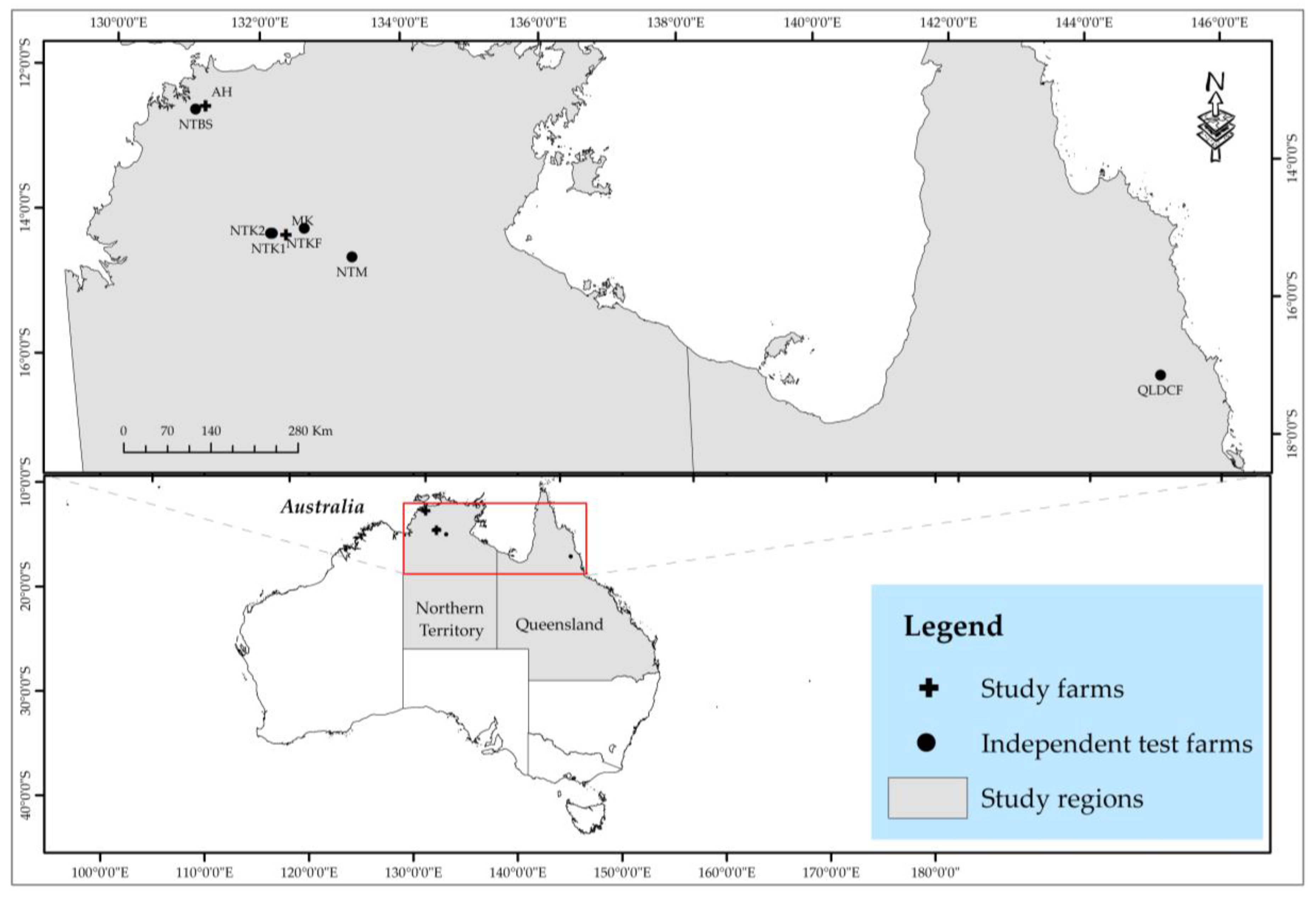
Figure 1. Location map showing the study farms and the independent test farms for model development and validation in the Northern Territory and Queensland, Australia.
Remotesensing 15 03075 g001
Figure 2. Yield distribution from 2015 to 2022 for the study farms (AH and MK).
Remotesensing 15 03075 g002
Figure 3. Distribution of rainfall and temperature in the study farm regions from 2015 to 2022. (Data Source: SILO platform (https://www.longpaddock.qld.gov.au/silo) (accessed on 5 June 2023)).
Remotesensing 15 03075 g003
Figure 4. Annual average GNDVI for: (a) Each study farm; and (b) independent test farms.
Remotesensing 15 03075 g004
Figure 5. A schematic representation of period year aggregation in relation to phenology stages for the 2017 prediction year.
Remotesensing 15 03075 g005
Figure 6. Correlation coefficients (different size circles) among yield and 16 best individual predictors selected based on the strength of the correlation at p < 0.05. Insignificant relationships are marked with an (×) and the color ramp shows the direction of the correlation.
Remotesensing 15 03075 g006
Figure 7. Performances of the six trialed ML algorithms in the individual (a) MK farm and (b) AH farm, as well as (c) the two farms combined model using only RS variables to predict yield at the block level.
Remotesensing 15 03075 g007
Figure 8. RS-based RF model predicted yield for: (a) MK farm; (b) AH farm; (c) combined farms model. The secondary y-axis shows the errors (%) associated with the predictions across the time series (2015–2022).
Remotesensing 15 03075 g008
Figure 9. Performances of the six trialed algorithms in: (a) The individual MK farm; (b) the individual AH farm; (c) the two farms combined model, using RS and weather variables to predict yield at the block-level.
Remotesensing 15 03075 g009
Figure 10. Predicting AH farm yield from: (a) A combined model; (b) a single farm model. Plots on the (left) and (right) show the training and test models, respectively. The red line and black dots represent the regression line of fit and the data points respectively.
Remotesensing 15 03075 g010
Figure 11. Actual and predicted production from the RS-based RF model validated on independent test farm locations in the Northern Territory and Queensland.
Remotesensing 15 03075 g011
Figure 12. Independent test farms validation (a) best and (b) worst performing models from the RS-based RF model. The (left) and (right) plots represent the training and test models, respectively. The validation point (n = 6) was obtained from the aggregation of 96 orchard blocks. The red line and black dots represent the regression line of fit and the data points respectively.
Remotesensing 15 03075 g012
Figure 13. Comparing errors associated with different training dataset sizes using models trained with 100 bootstrap samples per training dataset size. Model performance indicated in: (a) R2; (b) MAE; (c) RMSE.
Remotesensing 15 03075 g013
Table 1. Existing research using ML algorithms for crop yield prediction.
CropAlgorithm/MethodRS PlatformAccuracyResearch SummaryReference
GrapeGaussian process regressionUAV85.95%Evaluated both traditional linear and ML regressions to forecast in-season grape yield[15]
MangoFully Convolutional Network (FCN)RGB Camera73.6%Used MangoNet, a deep CNN based architecture for mango detection using semantic segmentation[41]
MangoLinear RegressionWorld View-3 satellite imagery>90%Predicted in-season infield mango yield for one season with the 18-tree calibration approach using high resolution RS imagery [26]
RiceANN, KNN, SVR and RF-86.5%Evaluated the performance of the four ML algorithms and to assess the importance of distinct feature sets on the ML algorithms[42]
CitrusRegion Convolutional Neural Network
(Faster R-CNN)
Vehicle mounted camera (FLIR A655SC)96%Detected and counted fruits using a combination of a thermal imaging methods and ML to tackle problems associated with color similarity between immature citrus and leaves.[43]
AppleFaster R-CNNUAV>90%Detected small target fruits from top-view RGB images of apple trees from UAV captures[44]
Table 2. Summary of grower data obtained from the AH and MK farms in the NT.
FarmLocationCultivarNo. of BlocksAvg. Blk Size (ha)Avg. Yield (t/ha)Period
(Yr)
Age (Yr)Spacing (m)Total No. of
Data Points
MKNTKP315.88.32015–2021236 × 9214
R2E295.99.0188 × 1362
AHNTCAL1112.114.12015–2020, 202223variable74
Combined 351 8 350
Table 3. Vegetation indices used in this study.
Vegetation IndexFormulaReference
Normalized Difference Vegetation Index (NDVI)(NIR − R)/(NIR + R)Rouse Jr et al. [54]
Green Normalized Difference Vegetation Index (GNDVI)(NIR − G)/(NIR + G)Gitelson et al. [55]
Enhanced Vegetation Index (EVI)2.5 × ((NIR − R)/(L + NIR + C1 × R − C2 × B))Huete et al. [56]
Land Surface Water Index (LSWI), also known as the Normalized Difference Water Index (NDWI)(NIR − SWIR2)/(NIR + SWIR2)Chandrasekar et al. [57]
Gao [58]
Table 4. Description of remote sensing (VI) and weather (WV) predictor variables for the current year (y0—prediction year), previous year (y1—1 year prior to prediction), and two previous years (y2—two years prior to the prediction year).
Predictor Variable NameCodeDescription
Period 1 of current year’s VIVI_p1_y0Median value of the VI of Period 1 of the current year
Period 2 of current year’s VIVI_p2_y0Median value of the VI of Period 2 of the current year
Period 1 of last year’s VIVI_p1_y1Median value of the VI of Period 1 of the previous year
Period 2 of last year’s VIVI_p2_y1Median value of the VI of Period 2 of the previous year
Period 3 of last year’s VIVI_p3_y1Median value of the VI of Period 3 of the previous year
Period 1 of last 2 year’s VIVI_p1_y2Median value of the VI of Period 1 of the last 2 years
Period 2 of last 2 year’s VIVI_p2_y2Median value of the VI of Period 2 of the last 2 years
Period 3 of last 2 year’s VIVI_p3_y2Median value of the VI of Period 3 of the last 2 years
Period 1 of current year’s WVWV_p1_y0Median value of the WV of Period 1 of the current year
Period 2 of current year’s WVWV_p2_y0Median value of the WV of Period 2 of the current year
Period 1 of last year’s WVWV_p1_y1Median value of the WV of Period 1 of the previous year
Period 2 of last year’s WVWV_p2_y1Median value of the WV of Period 2 of the previous year
Period 3 of last year’s WVWV_p3_y1Median value of the WV of Period 3 of the previous year
Period 1 of last 2 year’s WVWV_p1_y2Median value of the WV of Period 1 of last 2 years
Period 2 of last 2 year’s WVWV_p2_y2Median value of the WV of Period 2 of last 2 years
Period 3 of last 2 year’s WVWV_p3_y2Median value of the WV of Period 3 of last 2 years
Table 5. Description of relevant hyperparameters of the machine learning algorithms trialed with their typical range of values.
AlgorithmHyperparameter Function/DescriptionReference
RF
  • mtry controls the number of predictors sampled randomly on each node split. Range (2—√(n)), where n is the number of predictors and √ is square root.
  • ntree controls the total number of independent trees grown, range (50–500).
  • max_depth controls the maximum depth of a tree, range (0–10)
Breiman [64]
Jeong et al. [34]
Freeman et al. [37]
Kuhn [60]
SVR
  • Cost is the regularization parameter that allows weight assignment. Range (0,1).
  • Sigma defines the kernel function parameter (e.g., svmRadial, Gaussian or linear), range (0–0.07).
Brdar, et al. [35]
Kuhn [60]
XGBOOST
  • eta is also known as learning rate. It is a term that shrinks feature weights making the boosting process conservative—avoiding overfitting, range (0.3–0.4).
  • max_depth is the maximum depth of a tree. Increasing it makes the model complex and likely to overfit, range (2–3).
  • min_child_weight is the minimum sum of instance weight needed in a child. Larger values make the algorithm more conservative, range (0,1).
  • subsample selects a subsample of the training data in each iteration helping to prevent overfitting, range (0.5–1).
Chen and Guestrin [36]
Kuhn [60]
PLSR
  • ncomp is the number of partial least square components, range (6–20).
Hastie et al. [65]
Mevik and Wehrens [62]
RIDGE
  • Lambda is the L2 regularization term on weights to reduce overfitting, range (0,1).
Hastie et al. [61]
Aarshay [66]
LASSO
  • Lambda is the L1 regularization term on weights to reduce overfitting and also to improve algorithm performance for very high dimensionality data, range (0,1).
Hastie et al. [61]
Aarshay [66]
Table 6. RF-based model percentage error (NMAE, Equation (3)) at the block level and farm level (FLEM, Equation (4)) from only RS variables.
Error (%)20152016201720182019202020212022
Block level38.546.746.256.337.455.738.426.3
Farm level4.3538.626.730.9154.315.3
Table 7. RF-based model percentage error (NMAE) at the block level and the farm level (FLEM) from a combination of RS and weather variables for the combined farms model.
Error (%)20152016201720182019202020212022
Block level37.447.166.170.728.750.933.644.5
Farm level8.86.282.746.7225.23.739.4
Disclaimer/Publisher’s Note: The statements, opinions and data contained in all publications are solely those of the individual author(s) and contributor(s) and not of MDPI and/or the editor(s). MDPI and/or the editor(s) disclaim responsibility for any injury to people or property resulting from any ideas, methods, instructions or products referred to in the content.