Abstract
Diffuse attenuation coefficient of photosynthetically available radiation (PAR), KPAR, is a key product of ocean color remote sensing. Current ocean color algorithms generally detect only the average KPAR within one optical depth, . Due to the marked vertical variations of KPAR, knowledge of is insufficient to accurately evaluate the submarine light field. By using field in situ observations, a two-step approach, based on the development of an ocean color algorithm for and the relationships between and the average KPAR from the surface down to depth Z (), was developed to remotely estimate the vertical variations in in the North Pacific from the MODerate-resolution Imaging Spectrometer (MODIS) imagery. The root mean square difference of log() in depths within the euphotic zone was around ±0.059 (in unit of m−1 for ), which corresponded to a deviation of ±15% for the estimated and the penetration depths of PAR. Our study may provide a promising approach to detect the vertical variations of and underwater PAR distributions in the North Pacific Ocean.
1. Introduction
Knowledge of the vertical distribution of photosynthetically available radiation (PAR), which is associated with approximately the visible part of the solar radiation spectrum from 400 to 700 nm, is essential to understanding the underwater biogeochemical processes and the response of marine ecosystem to environmental changes [1,2]. Playing a key role in driving water-column photosynthesis, the vertical distribution of PAR, especially in the euphotic layer, is needed for accurately quantifying and modeling the aquatic primary production, which, as a whole for the global oceans, accounts for about half of global carbon fixation and thus alters the global oxygen and carbon balances [3,4,5]. In addition to being a controlling factor in the water-column photosynthesis, the vertical distribution of PAR is fundamental to predictions of vertical subsurface heating rates, given that more than 98% of total incoming solar irradiance as short wave is converted to heat. Subsurface heating can lead to instabilities of the upper layer, which in turn affects the physical and biogeochemical processes and photo-oxidation in the water column [6,7]. Moreover, the status of the penetration of PAR is often applied to evaluate the water clarity, which is an important environmental driver in benthic communities such as seagrass and coral reefs [8,9]. Nevertheless, an improvement will be realized in predicting climate changes and monitoring water quality with the improvement in the assessment of the vertical distribution of PAR.
According to the Lambert–Beer Law, PAR decreases approximately exponentially with depth (Z) and can be expressed as follows [1,10,11,12,13,14,15]:
where PAR(Z) and PAR(0−) are the PAR values at depth Z and just below the surface, respectively, while represents the average diffuse attenuation coefficient of the PAR (KPAR) from the surface down to depth Z. Since PAR(0−) can be modeled accurately [16], the determination of PAR(Z) is dependent almost exclusively on the accurate estimation of . As an apparent optical property (AOP), however, KPAR, as well as , is dependent on not only the water-column inherent optical properties (IOPs) such as absorption and scattering coefficients of water components, but also the angular structure of the submarine light field [11]. As such, KPAR is pronouncedly depth-dependent, varying by even more than a factor of two in the euphotic zone [10,12,13,17].
KPAR, and thus , can be measured in situ relatively simply, but such data are severely limited in their spatial and temporal coverage. On the other hand, satellite remote sensing provides a synoptic, large-scale, and continuous view of the oceans to augment the direct field in situ observations [18]. Efforts were made in past decades to develop and validate ocean color algorithms for KPAR [10,12,19,20,21]. Three types of algorithms are commonly developed for remotely estimating KPAR: chlorophyll-based approach [12,19,22], IOP-based approach [10,13], and empirical algorithm based on the band ratios of remote sensing reflectance (Rrs) [20]. The first two types require remote sensing products, e.g., chlorophyll a (Chl_a) concentration and IOPs of absorption and backscattering coefficients, respectively. An additional uncertainty is likely introduced when propagating these products to estimate KPAR. Furthermore, the vertical variations in Chl_a and IOPs, especially in stratified waters, may also cause difficulty in evaluating the vertical distributions in KPAR [10,22].
The third type, namely, the Rrs-based empirical algorithm, has been routinely used to estimate the diffuse attenuation coefficients in the global oceans from space [20]. For historic reasons, algorithms for the diffuse attenuation coefficient of downwelling plane irradiance at 490 nm (K490), rather than KPAR, are commonly developed [20,21]. For example, the remotely sensed K490 () by the MODerate-resolution Imaging Spectrometer on Aqua (MODIS-Aqua) is estimated as
where X = log[Rrs(488)/Rrs(555)]. In order to convert to the remotely sensed KPAR (), an empirical algorithm is commonly used such that [12]
Although the combination of Equations (2) and (3) provides an operational approach to estimate from the MODIS-Aqua imagery, two questions are raised when applying it to evaluate the vertical distributions in KPAR. First, this approach requires the estimation of , and an additional uncertainty may be introduced when propagating to estimate . Secondly, there exists a gap between and the vertical variations in KPAR. is approximately equal to , the average KPAR from the surface down to one optical depth at which PAR is reduced to about 37% (e−1 ≈ 37%) of its surface value [13], since more than 90% of water-leaving radiance is reflected from the upper one optical depth [23]. is thus valid to evaluate the penetration of PAR in the layer above one optical depth only. Even with vertically uniform profiles of IOPs, KPAR can vary by a factor of two; thus, its value below one optical depth may be much lower than [10,13]. As such, the penetration depths of PAR in the lower layer may be substantially underestimation if using a constant KPAR equal to for the whole water column. Therefore, the relationship between and , in addition to the ocean color algorithms for , has to be elucidated in order to accurately quantify the submarine penetration of PAR from space. Although previous works have reported the estimations of on few specific layers, e.g., from the surface down to the base of the euphotic zone [10,14,15,17] or two optical depths [12], an approach to evaluate the vertical profiling in continuously has seldom been documented [22].
In this study, we report an attempt to develop an operational approach for remotely estimating the vertical distributions of in the oceanic water by using field observations collected in the North Pacific (Figure 1). The approach was designed in a two-step method: (1) to develop an algorithm for estimating directly from the Rrs band ratio, and (2) to build the relationships between and . Section 2 describes the data and methods employed in this study. Section 3 shows the results and discusses them in terms of algorithm development and validation. Section 4 shows the application of the algorithms in evaluating the distributional patterns of in the North Pacific. Section 5 draws the conclusions.
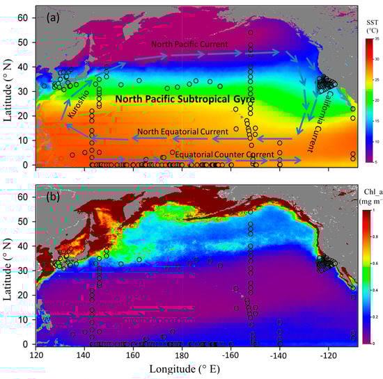
Figure 1.
Climatologically (2002–2022) seasonal variations in spring (21 March to 20 June) in the MODIS-Aqua-derived (a) sea surface temperature (SST) and (b) concentration of chlorophyll a (Chl_a) in the North Pacific. ○: field optical stations. Arrows show the major currents in the North Pacific.
2. Data and Methods
2.1. Study Area
The general distributional patterns of the biophysical properties, as shown in the climatologically seasonal distributions in spring in the MODIS-Aqua-derived sea surface temperature (SST) and Chl_a, in the North Pacific are shown in Figure 1. SST generally increases southwards from ~4 °C at 50°N to ~29 °C at the equator, primarily reflecting the latitudinal dependence of heat loss/gain across the air–sea interface. The major circulations, namely, the Kuroshio, the North Pacific Current, the California Current, and the North Equatorial Current, define the approximate boundaries of the North Pacific Subtropical Gyre (NPSG), which is the most extensive gyre of the Earth. The SSTs at the north and south boundaries of the NPSG are about 15 °C and 28 °C, respectively (Figure 1a). Corresponding to the southward-increasing SST, which may indicate the strengthened vertical stratification and thus reduced nutrient supply for phytoplankton growth, Chl_a generally decreases southwards, varying from ~0.4 mg m−3 at 50°N to ~0.1 mg m−3 at the equator (Figure 1b). High Chl_a, e.g., over 1 mg m−3, can be found in the coastal waters, while the most oligotrophic waters are found in the NPSG, with Chl_a typically around 0.05 mg m−3. In terms of PAR, as exampled in its climatologically seasonal distribution in spring in the North Pacific (Figure A1 in Appendix A), it generally increases southwards from ~30 E m−2 d−1 at 50°N to ~45 E m−2 d−1 at the equator. Latitudinal maximum values of PAR typically occur at about 10–17°N. Seasonally, PAR generally increases from the winter to the summer, then following a decrease to the winter. Seasonal variations are typically more pronounced in the high-latitude region than in the low-latitude region. Such a distributional pattern may primarily reflect the spatial and temporal variability in the incoming total solar irradiance, in addition to modulation of the atmospheric transmission associated with cloud cover and aerosol distributions.
2.2. Field In Situ Observations in the Experiment of Pac_2017
A total of 65 stations, including 25 optical stations, covering from the equator to 40°N, 143 to 149°E, were occupied between 14 April and 13 May 2017 during the 2017 cruise of the Spring Voyage of the Comprehensive Survey of Water Bodies in the Central and Southern Western Pacific by R/V Kexue (Pac_2017; Figure 1; Table 1). At each station, vertical distributions of water temperature and salinity were recorded with a SeaBird SBE9/11 conductivity–temperature–depth (CTD) recorder. The mixed layer depth (MLD) was defined as the depth at which the temperature was 0.5 °C lower than the surface temperature [24]. Discrete water samples were collected with depth by using 20 L SBE bottles mounted onto a Rosette sampling assembly. Samples for the determination of the concentrations of Chl_a were collected through 47 mm GF/F Whatman glass fiber filters by filtering ~2.5 L seawater onboard the ship. The concentrations of Chl_a were determined by fluorimetry [25], though such a historically widely used technique may produce a relatively high uncertainty in determining Chl_a, e.g., tending to underestimate Chl_a when chlorophyll b is unusually distributed in the water. Only the surface concentrations of Chl_a, whose samples were collected at 10 m depth, are reported here.

Table 1.
Field experiments used for this study. Detailed sampling dates for experiments can be found in the Appendix A (Table A1).
At each optical station conducted in the daytime, vertical profiling of the spectral downwelling irradiance [Ed(λ, Z)] and upwelling radiance [Lu(λ, Z)], along with simultaneous measurements of the sea surface solar irradiance [Es(λ)], between 400 and 700 nm in 2 nm intervals was determined through a Satlantic HyperPro II system by following the manufacturer’s manual (https://www.seabird.com/hyperpro-ii/product-downloads?id=54627923897 (accessed on 1 December 2021)). PAR(Z) (µE m−2 s−1) was calculated as follows:
where λ (nm), Z (m), and Ed(λ, Z) (µW cm−2 nm−1) represent light wavelength, water depth, and spectral downwelling irradiance at depth Z, while h, c, and NA are the Planck’s constant (6.625 × 10⁻³⁴ J s), the speed of light (3 × 10⁸ m s−1), and the Avogadro constant (6.022 × 10²³ mol−1), respectively. The euphotic zonal depth (EZD) was defined as the depth at which PAR(Z) was 1% of the surface value. According to Equation (1), (in unit of m−1) was calculated as . The above-water spectral remote sensing reflectance [Rrs(λ)] was determined from Ed(λ, Z), Lu(λ, Z), and Es(λ) using a data processor in compliance with the Ocean Optics Protocols established for in situ observations in support of ocean color remote sensing measurements [26].
2.3. Additional Field Datasets
Additional field observations in the North Pacific were downloaded from the Hawaii Ocean Time-Series (HOT) website (https://hahana.soest.hawaii.edu/hot/ (accessed on 1 December 2021)), in which optical observations conducted at the ALOHA (A Long-Term Oligotrophic Habitat Assessment) station (22.75°N, 158.00°W) between 2009 and 2019 were extracted, and the SeaWiFS Biooptical Archive and Storage System (SeaBASS; https://seabass.gsfc.nasa.gov/ (accessed on 1 December 2021)) [27], in which optical observations conducted in multiple cruises were extracted (Figure 1; Table 1). The extracted data included PAR(Z), Ed(λ, Z), Lu(λ, Z), and Es(λ). Similarly, and Rrs(λ) were determined from these observations by following the methods as used in Section 2.2. To reduce the effect of the variation of the incident solar light on accurately determining and Rrs(λ), e.g., overpassing clouds might markedly reduce the incoming PAR(0−) and thus PAR(Z), casts whose coefficients of variation in Es(λ) during sampling were >1% were excluded. Then, 745 sets of observations in and Rrs(λ) were available.
The extracted data were pooled into our observations, and, finally, there were 770 sets of observations. About 80% (617) of stations, which were randomly selected by using Excel® “Rand” function, were used for algorithm development, and the remaining 20% (153) of stations were used to validate the algorithms.
2.4. Statistics
The performance of the algorithm of the remotely sensed and the penetration depth of PAR was evaluated by the root mean square difference (RMSD) such that
where n, F, and D are the number of samples, the observations, and the corresponding derived products, respectively. Unless noted, uncertainty used in this study means RMSD.
3. Results
3.1. Hydrographic Properties Observed In Situ
The in situ observations followed similar patterns to the remotely sensed data (Figure 1), as exampled in the latitudinal variations of SST, surface salinity, MLD, EZD, and surface Chl_a along 143–149°E observed during our cruise (Pac_2017) conducted in April–May 2017 (Figure 2). According to reports in the literature [28,29,30,31,32,33], this area might be subdivided into three primary hydrographic regimes, the Kuroshio Extension (north of 34°N), the NPSG (15–25°N) and the western Tropical Pacific (south of 10°N), and two transition zones (25–34°N and 10–15°N). The SST, 14.2 ± 3.0, 27.0 ± 1.5, and 29.9 ± 0.4 °C in the Kuroshio Extension, the NPSG, and the western Tropical Pacific, respectively, increased southwards. Surface salinity generally increased from 34.6 ± 0.2 in the Kuroshio Extension to 34.9 ± 0.3 in the NPSG and then decreased to 34.0 ± 0.2 in the western Tropical Pacific, consistent with previous reports [34,35]. The MLD, 138 ± 72 m, was deep and was much deeper than the EZD, 53 ± 21 m, in the Kuroshio Extension, suggesting a replete supply of nutrients by vertical mixing and thus resulting in a large surface Chl_a, 1.12 ± 0.30 mg m−3. In the NPSG, as reported in the literature [36], the MLD, 29 ± 10 m, became very shallow and was much shallower than the EZD, 115 ± 17 m. Because the permanent anticyclonic circulation leads to an Ekman downwelling, a deep pycnocline, and a limited supply of nutrients by vertical mixing [36,37], the surface Chl_a, 0.07 ± 0.02 mg m−3, was very low in the NPSG. In the western Tropical Pacific, the MLD, 76 ± 20 m, was shallower than the EZD, 103 ± 16 m, and the surface Chl_a, 0.07 ± 0.02 mg m−3, was also low. Nevertheless, the MLD, the EZD, and the surface Chl_a were all significantly (p < 0.01) correlated with the SST (r = −0.53, 0.88, and −0.84), suggesting that the temperature-associated status of water stratification is important, if not dominant, in controlling the distributions of the physical, hydrographic, and biological qualities in the North Pacific.
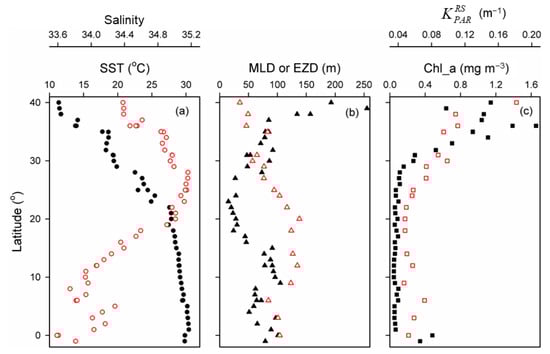
Figure 2.
Latitudinal variations in (a) SST (●) and surface salinity (○), (b) mixed layer depth (MLD, ▲) and euphotic zonal depth (EZD, ∆), and (c) surface Chl_a (■) and calculated remotely sensed diffuse attenuate coefficient of PAR (, □) along 143–149°E observed in situ during the Pac_2017 cruise.
3.2. Variations of KPAR Observed In Situ
Horizontal variations of KPAR, as exampled in the latitudinal variations of calculated from the in situ PAR observations in the first optical depth during the Pac_2017 cruise in April–May 2017, are shown in Figure 2c. Ranging between 0.05 and 0.18 m−1, generally decreased southward, following a similar trend to the surface Chl_a. In actuality, a positive correlation (r = 0.77) was found between and the surface Chl_a, suggesting that this study area is well classed into the Case-1 waters in which the optical properties are determined primarily by the phytoplankton and their associated living and inanimate materials.
Depth-dependence in was pronounced in all water conditions. Vertical variations of PAR(Z)/PAR(0−) and , as exampled in a well-mixed station (149°E, 38°N) and a stratified station in the NPSG (143°E, 22°N) during the Pac_2017 cruise, are shown in Figure 3. More examples can be found in the Appendix A (Figure A2). At both stations, although PAR(Z)/PAR(0−) followed a generally exponential decay function with depth, it was reduced faster in the upper layer than in the lower layer, resulting in a generally decreasing with depth, consistent with previous reports [10,12,13,17]. In the well-mixed station, , ranging between 0.115 and 0.094 m−1, varied by a factor of 1.2 (Figure 3a). In the stratified station, , ranging between 0.056 and 0.038 m−1, varied by a factor of 1.5 (Figure 3b). Without considering the vertical variations in , i.e., by treating vertically constant to , the penetration depths of PAR would be markedly underestimated. For example, the estimated EZDs by using constant equal to were 42 and 92 m, which were shallower than the observations of 49 and 117 m by 14% and 21% in these two stations (Figure 3). These results indicated that knowing alone is insufficient to retrieve the submarine penetration of PAR. In order to accurately estimate the penetration depths of PAR at different light levels from space, the relationships between and have to be built.
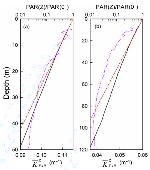
Figure 3.
Vertical variations of PAR(Z)/PAR(0−) (black solid lines) and (pink dash–dotted lines) in (a) a well-mixed station (149°E, 38°N) and (b) a stratified station (143°E, 22°N) during the Pac_2017 cruise. The estimated PAR(Z)/PAR(0−) by treating vertically constant to are shown using the red dashed lines.
3.3. Algorithm Development for Remotely Sensing in the North Pacific
In this study, we adapted a two-step method for remotely estimating : developing an ocean color algorithm for , and building the relationships between and . For the first step, could be related to Rrs band ratio such that (Figure 4)
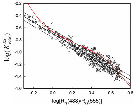
Figure 4.
Relationship between log() and log[Rrs(488)/Rrs(555)] for data used for algorithm development. is given in unit of m−1. Black solid line—best fit line of Equation (6); dashed lines—one RMSD (±0.065) from the best fit line; red solid line—relationship by using the combined Equations (2) and (3).
Again, X = log[Rrs(488)/Rrs(555)]. The RMSD of the derived log() was ±0.065 (in unit of m−1 for ), which corresponded to a deviation of about ±16% in the derived . This uncertainty was reduced to 2/3 of that by applying the commonly used approach, the combined Equations of (2) and (3), which introduced the RMSD of ±0.103 in the derived log() and the corresponding deviation of about ±27% in . Moreover, the use of the combined Equations (2) and (3) generally introduced an overestimation on .
For the second step, our data indicated that for a given light level (f) within the euphotic zone whose corresponding depth is Zf so that f = PAR(Zf)/PAR(0−) × 100%, the average KPAR from the surface down to Zf, , could be linearly related to (r2 > 0.96; Figure 5), while the derived slope (A) was related to log(f) by a third-order polynomial function such that (r2 = 0.996; Figure 6)
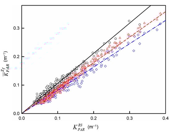
Figure 5.
Linear regressions between and for selected light levels of f = 50% (○, solid black line), 10% (∆, dashed red line), and 1% (◊, dot–dashed blue line) for data used for algorithm development.
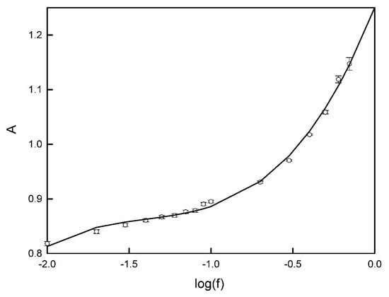
Figure 6.
Relationship between the slope of Equation (7) (A, ○) and light level (f). Symbols (○) and error bars represent the regressed A values and the standard deviations.
The RMSD of log() derived from Equation (7) was around ±0.041 (ranging between ±0.015 and ±0.055 for f varying from 1% to 70%; in unit of m−1), resulting in the corresponding deviation of the derived to be around ±10%. By definition,
Zf could thus be determined such that
By combining Equations (6) and (7), given the light level of f, could be determined from the Rrs band ratio, and the corresponding Zf could then be further determined from Equation (10). The RMSD of log() derived from this approach was around ±0.059 ( in unit of m−1), which corresponded to a deviation of ±15% in both the derived (Figure 7a) and Zf (Figure 7b). The above results suggest that, given substantially accurate Rrs spectra by satellites, the remote estimates in and Zf at any light levels within the euphotic zone could be accurately estimated from space with a deviation of ±15% only.
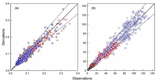
Figure 7.
Comparisons of the derived (a) (m−1) and (b) the associated penetration depths (Zf, m) by using our approach with the field in situ observations for selected light levels of f = 50% (○), 10% (∆), and 1% (◊) for data used for algorithm development. Solid lines—1:1 plots; dashed lines—±15% deviated from the 1:1 plots.
3.4. Validation on the Derived
The performance of the proposed approach was further validated by comparing and Zf derived from Rrs(λ) to the observations in the dataset used for validation. The resulting RMSD in log() for light levels within the euphotic zone was around ±0.057 ( in unit of m−1), which corresponded to a deviation of ±14% in both the derived (Figure 8a) and Zf (Figure 8b). These values were even slightly smaller than those found in the algorithm development, suggesting that there was a general good agreement on the remotely sensed and the observed and Zf.
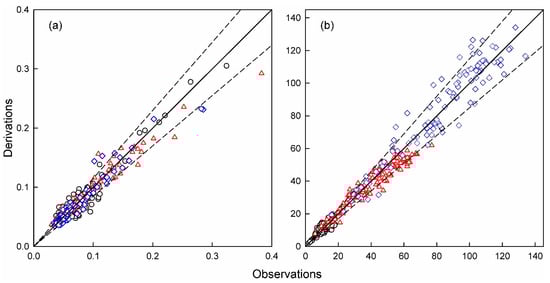
Figure 8.
The same as Figure 7 but for in situ data used for validation. (a) (m−1) and (b) the associated penetration depths (Zf, m).
Comparisons of the MODIS-Aqua-derived and Zf to the field in situ observations, by following the protocols [38], are shown in Figure 9. For each station, the main criteria included minimum 5 valid pixels in the 3 × 3 pixel array centered on the field station, coefficient of variation of valid satellite pixels lower than 0.15, and time difference within ±3 h between satellite overpass and field observation. The resulting RMSD in log() for light levels within the euphotic zone was around ±0.073 ( in unit of m−1), which corresponded to a deviation of ±18% in both the derived (Figure 9a) and Zf (Figure 9b). These values were slightly larger but still quite comparable to those found in Figure 7 and Figure 8, suggesting that there was a reasonable agreement between the remotely sensed and the observed and Zf. Nevertheless, since only 13 match-up data points were available for this evaluation, further validation when additional field observations became available would be desirable.
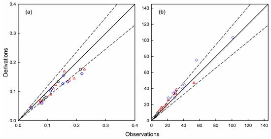
Figure 9.
The same as Figure 7 but the derivations were made from the MODIS-Aqua match-up data with a satellite overpass time window of ±3 h. Here, dashed lines represent ±18% deviated from the 1:1 plots (solid lines). (a) (m−1) and (b) the associated penetration depths (Zf, m).
4. Application: Distributions of Remotely Sensed and Zf in the North Pacific
The operational approach developed in this study can be applied to estimate the vertical variations of KPAR from space. Using MODIS-Aqua monthly Level-3 products (Reprocessing R2022.0) of Rrs(488) and Rrs(555) extracted from the NASA Ocean Color Web (http://oceancolor.gsfc.nasa.gov (accessed on 1 December 2022)), the climatologically (2002–2022) seasonal distributions in spring in the satellite-derived , , and EZD in the North Pacific are shown as examples in Figure 10. is generally >0.1 m−1 north of 40°N, typically <0.05 m−1 in the NPSG, and around 0.06 m−1 south of the NPSG (Figure 10a). Such a distributional pattern generally follows the pattern of the latitudinal variations in SST (Figure 1a) such that high is associated with low SST and vice versa. Enhanced nutrient supply and, hence, primary production by vertical mixing to the surface layer in low SST (Figure 2) may account for high in low-SST conditions. High values of can also be found in the coastal waters, in which land-sourced inputs and/or southward currents are marked, and in the cyclonic circulation gyres, e.g., region surrounded by the Oyashio, the North Pacific Current, and the Alaska Current at about 160°E–135°W, 40–60°N [32]. The upwelling may enhance vertical transport of nutrients to the surface layer to support phytoplankton growth, resulting in the increased turbidity and, thus, high . In contrast, the NPSG is characterized as oligotrophic waters with very low because of the occurrence of a permanent anticyclonic circulation gyre. is slightly enlarged south of the NPSG, possibly due to the slightly enhanced vertical mixing by the blowing of the trade winds [32]. , whose value is about 81% of , follows a similar distributional pattern to (Figure 10b). The distributional pattern in the EZD follows a reverse trend to (Figure 10c) according to Equation (9). As such, the EZD may vary from <50 m north of 40°N to >110 m in the NPSG.
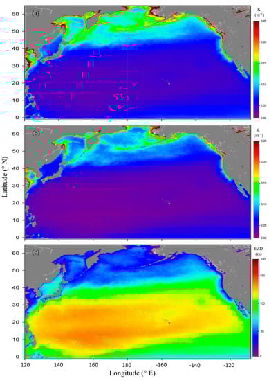
Figure 10.
Climatologically (2002–2022) seasonal distributions in spring in the MODIS-Aqua-derived (a) , (b) , and (c) EZD in the North Pacific.
The application of the remotely sensed and the associated vertical distributions of the PAR may improve the accuracy in the assessment of the carbon fixation in the North Pacific. For example, the remotely sensed net primary production in the euphotic zone (PPeu) is thought to be linearly related to the euphotic zonal depth (EZD) [5]. The EZD is typically underestimated, e.g., by 14 ± 16% using the models integrated in the PPeu model [5] or by 16 ± 11% estimated by treating vertically constant to (Figure 3 and Figure A2). As a result, PPeu may be substantially underestimated in the North Pacific. A reassessment on the contribution of the North Pacific to the global carbon cycle may be needed.
Although an improved approach to remotely estimate in the North Pacific has been proposed in this study, it is necessary to note that it is designed to be applied to the Case-1 waters, given that most of the in situ observations were conducted in the offshore regions. For inshore locations and marginal seas at land–sea boundaries, which are typically characterized as the Case-2 waters, regionally tuned algorithms are generally needed.
5. Conclusions
This study demonstrated that, by adapting a two-step approach, that is, developing an ocean color algorithm for and building the relationships between and , the vertical variations in in the North Pacific may be assessed from space. The deviation in the remotely sensed in depths within the euphotic zone, as well as the corresponding penetration depths of PAR, is about ±15%. The significant underestimation in the remotely sensed euphotic zonal depth from methods adapted in current primary production models suggests a substantial underestimation of the primary production in the North Pacific. The variations in , together with those in other hydrographic properties (e.g., SST and Chl_a), suggest that our dataset covers various water conditions and, thus, may be a good representative to the Case-1 waters in the North Pacific Ocean. A similar approach may be developed for the global oceans when field observations in the global oceans become available.
Author Contributions
Conceptualization, X.P. and L.C.; methodology, X.P. and J.Z.; software, L.C. and P.S.; validation, X.P., L.C. and J.Z.; formal analysis, L.C. and X.Z.; investigation, L.C. and X.Z.; resources, X.P.; data curation, X.P.; writing—original draft preparation, L.C.; writing—review and editing, X.P.; visualization, L.C.; supervision, J.Z.; project administration, P.S.; funding acquisition, J.Z. All authors have read and agreed to the published version of the manuscript.
Funding
This research was funded by Finance Science and Technology Project of Hainan Province, grant number ZDYF2021GXJS037; National Natural Science Foundation of China, grant number 42266005, 61931025 and U1906217; Major Science and Technology Plan Project of Hainan Province, grant number ZDKJ202017-02-01; Key Deployment Project of Centre for Ocean Mega-Research of Science, Chinese Academy of Sciences, grant number COMS2019Q05; Scientific Research Foundation of Hainan Tropical Ocean University, grant number RHDRC202103; Spring Voyage of the Comprehensive Survey of Water Bodies in the Central and Southern Western Pacific, grant number GASI-02-pac-stmsspr.
Data Availability Statement
Data from this research will be available upon request to the authors.
Acknowledgments
The authors thank the captain and the crew of R/V Kexue that assisted in sample collection.
Conflicts of Interest
The authors declare no conflict of interest.
Appendix A
Table A1.
Sampling dates for the field experiments used for this study.
Table A1.
Sampling dates for the field experiments used for this study.
| Experiments | Periods |
|---|---|
| W_Pacific | 14 Apr–13 May 2017 |
| HOT | 24 Sep, 3 Nov, 9 Dec 2009; 6 Apr, 18 May, 8 Jul, 3 Sep, 3 Oct 2010; 11 Apr, 27 Sep, 4 Nov, 29 Nov, 18 Dec 2011; 18 Jan, 1 May, 30 May, 14 Sep, 7 Oct, 3 Dec 2012; 6 Mar, 5 Apr, 17 May, 11 Sep, 27 Oct, 26 Nov 2013; 5 Mar, 10 Apr, 1 Jun, 30 Jun, 13 Oct 2014; 28 Mar, 21 Apr, 23 May, 19 Jun, 19 Jul, 12 Aug, 13 Oct, 8 Dec 2015; 9 Feb, 15 Apr, 29 Nov 2016; 24 Jan, 23 Feb, 25 Apr, 20 Jun 2017; 18 Apr, 10 Sep, 14 Oct 2018; 20 Feb, 4 May, 13 Jun, 1 Jul 2019 |
| ACE-Asia | 18 Mar–17 Apr 2001 |
| CalCOFI | 14–23 Aug, 19–24 Oct 1993; 20 Jan–5 Feb, 22 Mar–7 Apr, 6–19 Aug, 30 Sep–14 Oct, 1994; 6–21 Apr, 6–19 Jul, 12–25 Oct 1995; 30 Jan–10 Feb, 16–24 Apr, 10 Oct–1 Nov 1996; 30 Jan–14 Feb, 6–16 Apr, 2–15 Jul, 20 Sep–5 Oct 1997; 23 Jan–10 Feb, 3–20 Apr, 16–26 Jul, 13–26 Sep 1998; 10–19 Aug, 3–18 Oct 1999;7–26 Jan 2000; 10-16 Jul 2001; 3–12 Jul, 16–17 Nov 2002; 7–22 Apr 2003; 2–18 Nov 2004 |
| CCE_LTER | 11–20 May 2006; 4–19 Apr 2007; 5–27 Oct 2008 |
| CLIVAR | 21 Feb–27 Mar 2006; 17–27 Dec 2007 |
| JGOFS | 20–21 Feb 1988; 25 Mar–14 Apr 1992 |
| JGOFS_WOCE | 16–28 Sep 1991 |
| OCEAN_LIDAR | 19–24 Nov, 1–12 Dec 1994; 26–30 Dec 1995; 7–14 Jan 1996; 9–17 Jan, 14 Nov–20 Dec 1997; 1–10 Feb 1998; 31 Dec 1998–15 Jan 1999; 20 Nov–6 Dec 1999; 12–29 Jan 2001 |
| ZonalFlux | 24 Apr–10 May 1996 |

Figure A1.
Climatologically (2002–2022) seasonal distributions in spring in the MODIS-Aqua-derived PAR.

Figure A2.
Latitudinal variations in the vertical variations of PAR(Z)/PAR(0−) (black solid lines) and (pink dash–dotted lines) along ~152°W for selected stations conducted in the CLIVAE experiment during 21 February to 27 March 2006. The estimated PAR(Z)/PAR(0−) by treating vertically constant to are shown in the red dashed lines. Latitudes for the stations are (a) 4°N; (b) 14°N; (c) 23°N; (d) 34°N; (e) 45°N; (f) 54°N.
References
- Kirk, J.T.O. Light and Phytosynthesis in Aquatic Ecosystems, 2nd ed.; Cambridge University Press: New York, NY, USA, 1994. [Google Scholar]
- Morel, A. Light and marine photosynthesis: A spectral model with geochemical and climatological implications. Prog. Oceanog. 1991, 26, 263–306. [Google Scholar] [CrossRef]
- Behrenfeld, M.J.; O’Malley, R.T.; Siegel, D.A.; McClain, C.R.; Sarmiento, J.L.; Feldman, G.C.; Milligan, A.J.; Falkowski, P.G.; Letelier, R.M.; Boss, E.S. Climate-driven trends in contemporary ocean productivity. Nature 2006, 444, 752–755. [Google Scholar] [CrossRef] [PubMed]
- Boyd, P.; Trull, T.W. Understanding the export of biogenic particles in oceanic waters: Is there consensus? Prog. Oceanogr. 2007, 72, 276–312. [Google Scholar] [CrossRef]
- Behrenfeld, M.J.; Falkowski, P.G. Photosynthetic rates derived from satellite-based chlorophyll concentration. Limnol. Oceanogr. 1997, 42, 1–20. [Google Scholar] [CrossRef]
- Chen, J.; Zhang, X.; Xing, X.; Ishizaka, J.; Yu, Z. A spectrally selective attenuation mechanism-based Kpar algorithm for biomass heating effect simulation in the open ocean. J. Geophys. Res. Oceans 2017, 122, 9370–9386. [Google Scholar] [CrossRef]
- Mobley, C.D.; Boss, E.S. Improved irradiances for use in ocean heating, primary production, and photo-oxidation calculations. Appl. Opt. 2012, 51, 6549–6560. [Google Scholar] [CrossRef]
- Xu, M.; Barnes, B.B.; Hu, C.; Carlson, P.R.; Yarbro, L.A. Water clarity monitoring in complex coastal environments: Leveraging seagrass light requirement toward more functional satellite ocean color algorithms. Remote Sens. Environ. 2023, 286, 113418. [Google Scholar] [CrossRef]
- Barnes, B.B.; Hallock, P.; Hu, C.; Muller-Karger, F.; Palandro, D.; Walter, C.; Zepp, R. Prediction of coral bleaching in the Florida Keys using remotely sensed data. Coral Reefs 2015, 34, 491–503. [Google Scholar] [CrossRef]
- Lee, Z.; Weidemann, A.; Kindle, J.; Arnone, R.; Carder, K.L.; Davis, C. Euphotic zone depth: Its derivation and implication to ocean-color remote sensing. J. Geophys. Res. 2007, 112, C03009. [Google Scholar] [CrossRef]
- Mobley, C. Light and Water: Radiative Transfer in Natural Waters; Elsevier: San Diego, CA, USA, 1994. [Google Scholar]
- Morel, A.; Huot, Y.; Gentili, B.; Werdell, P.J.; Hooker, S.B.; Franz, B.A. Examining the consistency of products derived from various ocean color sensors in open ocean (Case 1) waters in the perspective of a multi-sensor approach. Remote Sens. Environ. 2007, 111, 69–88. [Google Scholar] [CrossRef]
- Pan, X.; Zimmerman, R.C. Modeling the vertical distributions of downwelling plane irradiance and diffuse attenuation coefficient in optically deep waters. J. Geophys. Res. 2010, 115, C08016. [Google Scholar] [CrossRef]
- Son, S.; Wang, M. Diffuse attenuation coefficient of the photosynthetically available radiation Kd(PAR) for global open ocean and coastal waters. Remote Sens. Environ. 2015, 159, 250–258. [Google Scholar] [CrossRef]
- Wang, M.; Son, S.; Harding, L.W. Retrieval of diffuse attenuation coefficient in the Chesapeake Bay and turbid ocean regions for satellite ocean color applications. J. Geophys. Res. 2009, 114, C10011. [Google Scholar] [CrossRef]
- Gregg, W.W.; Carder, K.L. A simple spectral solar irradiance model for cloudless maritime atmospheres. Limnol. Oceanogr. 1990, 35, 1657–1675. [Google Scholar] [CrossRef]
- Lee, Z.; Hu, C.; Shang, S.; Du, K.; Lewis, M. Penetration of UV-visible solar radiation in the global oceans: Insights from ocean color remote sensing. J. Geophys. Res. 2013, 118, 4241–4255. [Google Scholar] [CrossRef]
- McClain, C.R. A decade of satellite ocean color observations. Ann. Rev. Mar. Sci. 2009, 1, 19–42. [Google Scholar] [CrossRef]
- Morel, A.; Berthon, J.-F. Surface pigments, algal biomass profiles, and potential production of the euphotic layer: Relationships reinvestigated in view of remote-sensing applications. Limnol. Oceanogr. 1989, 34, 1545–1562. [Google Scholar] [CrossRef]
- Mueller, J.L. SeaWiFS algorithm for the diffuse attenuation coefficient, K(490), using water-leaving radiances at 490 and 555 nm. In SeaWiFS Postlaunch Calibration and Validation Analyses; Hooker, S.B., Firestone, E.R., Eds.; NASA/TM-2000-206892; NASA Goddard Space Flight Center: Greenbelt, MD, USA, 2000; Volume 11. [Google Scholar]
- Signorini, S.R.; Hooker, S.B.; McClain, C.R. Bio-Optical and Geochemical Properties of the South Atlantic Subtropical Gyre; NASA/TM-2003-212253; NASA Goddard Space Flight Center: Greenbelt, MD, USA, 2000. [Google Scholar]
- Xing, X.; Boss, E. Chlorophyll-based model to estimate underwater photosynthetically available radiation for modeling, in-situ, and remote sensing applications. Geophys. Res. Lett. 2021, 48, e2020GL092189. [Google Scholar] [CrossRef]
- Gordon, H.R.; McCluney, W.R. Estimation of the depth of sunlight penetration in the sea for remote sensing. Appl. Optics 1975, 14, 413–416. [Google Scholar] [CrossRef]
- Levitus, S. Climatological Atlas of the World Ocean; NOAA Professional Paper 13; U.S. Department of Commerce: Rockville, MD, USA, 1982. [Google Scholar]
- Strickland, J.D.H.; Parsons, T.R. A Practical Handbook of Seawater Analysis, 2nd ed.; Bulletin 167; Fisheries Research Board of Canada: Ottawa, ON, Canada, 1972. [Google Scholar]
- Mueller, J.L.; Austin, R.W. Ocean optics protocols for SeaWiFS validation, revision 1. In SeaWiFS Technical Report Series; Hooker, S.B., Firestone, E.R., Acker, J.G., Eds.; NASA Technical Memorandum 104566; NASA Goddard Space Flight Center: Greenbelt, MD, USA, 1995; Volume 25. [Google Scholar]
- Werdell, P.J.; Fargion, G.S.; Mcclain, C.R.; Bailey, S.W. The seaWiFS bio-optical archive and storage system (SeaBASS): Current architecture and implementation. NASA Tech. 2002, 48, 1–45. [Google Scholar]
- Deser, C.; Alexander, M.A.; Xie, S.-P.; Phillips, A.S. Sea surface temperature variability: Patterns and mechanisms. Annu. Rev. Mar. Sci. 2010, 2, 115–143. [Google Scholar] [CrossRef]
- Karl, D.M. A sea of change: Biogeochemical variability in the North Pacific Subtropical Gyre. Ecosystems 1999, 2, 181–214. [Google Scholar] [CrossRef]
- Johnson, K.S.; Riser, S.C.; Karl, D.M. Nitrate supply from deep to near-surface waters of the North Pacific subtropical gyre. Nature 2010, 465, 1062–1065. [Google Scholar] [CrossRef] [PubMed]
- Hu, D.; Wu, L.; Cai, W.; Gupta, A.S.; Ganachaud, A.; Qiu, B.; Gordon, A.L.; Lin, X.; Chen, Z.; Hu, S.; et al. Pacific western boundary currents and their roles in climate. Nature 2015, 522, 299–308. [Google Scholar] [CrossRef]
- Mann, K.H.; Lazier, J.R.N. Dynamics of Marine Ecosystems: Biological-Physical Interactions in the Oceans, 2nd ed.; Blackwell Science: Malden, MA, USA, 1996. [Google Scholar]
- Tseng, Y.H.; Lin, H.; Chen, H.C.; Thompson, K.; Bentsen, M.; Böning, C.W.; Bozec, A.; Cassou, C.; Chassignet, E.; Chow, C.H.; et al. North and equatorial pacific ocean circulation in the CORE-II hindcast simulations. Ocean Model. 2016, 104, 143–170. [Google Scholar] [CrossRef]
- Boutin, J.; Vergely, J.-L.; Marchand, S.; D’Amico, F.; Hasson, A.; Kolodziejczyk, N.; Reul, N.; Reverdin, G.; Vialard, J. New SMOS sea surface salinity with reduced systematic errors and improved variability. Remote Sens. Environ. 2018, 214, 115–134. [Google Scholar] [CrossRef]
- Yasuda, I. Hydrographic structure and variability in the Kuroshio–Oyashio transition area. J. Oceanogr. 2003, 59, 389–402. [Google Scholar] [CrossRef]
- Church, M.J.; Lomas, M.W.; Muller-Karger, F. Sea change: Charting the course for biogeochemical ocean time-series research in a new millennium. Deep-Sea Res. II 2013, 93, 2–15. [Google Scholar] [CrossRef]
- Pan, X.; Wong, G.T.F.; Ho, T.-Y.; Tai, J.-H. Diel variability of vertical distributions of chlorophyll a at the SEATS and ALOHA stations: Implications on remote sensing interpretations. Int. J. Remote Sens. 2019, 40, 2916–2935. [Google Scholar] [CrossRef]
- Bailey, S.W.; Werdell, P.J. A multi-sensor approach for the on-orbit validation of ocean color satellite data products. Remote Sens. Environ. 2006, 102, 12–23. [Google Scholar] [CrossRef]
Disclaimer/Publisher’s Note: The statements, opinions and data contained in all publications are solely those of the individual author(s) and contributor(s) and not of MDPI and/or the editor(s). MDPI and/or the editor(s) disclaim responsibility for any injury to people or property resulting from any ideas, methods, instructions or products referred to in the content. |
© 2023 by the authors. Licensee MDPI, Basel, Switzerland. This article is an open access article distributed under the terms and conditions of the Creative Commons Attribution (CC BY) license (https://creativecommons.org/licenses/by/4.0/).