


Sentinel-1 SAR Images and Deep Learning for Water Body Mapping


Abstract
1. Introduction
2. Related Works
3. Materials and Methods
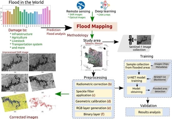
3.1. Study Area
3.1.1. Study Period
3.1.2. Image Acquisition
3.1.3. Preprocessing of SAR Images
- Radiometric correction. To correct the distortions of the radar signals caused by alterations in the movement of the sensor or instrument onboard the satellite. It should be noted that the intensity of the image pixels can be directly related to the backscatter signal captured by the sensor. Uncalibrated SAR images are helpful for qualitative use but must be calibrated for quantitative use. Figure 5a,b show an example of an image before and after correction.
- Speckle filter application. SAR images have inherent textures and dots that degrade image quality and make it challenging to interpret features. These points are caused by constructive and destructive random interference from coherent but out-of-phase return waves scattered by elements within each resolution cell. To provide a solution, speckle filtering was applied, with non-Gaussian multiplicative noise, which indicated that the pixel values did not follow a normal distribution. Consequently, the 7 × 7 Lee [87] filter was used to standardize the image and reduce this problem (see Figure 5c).
- Geometric calibration. SAR images may be distorted due to topographic changes in the scene and the inclination of the satellite sensor, which makes it necessary to reposition it. Data that do not point directly to the nadir position of the sensor will have some distortion. The digital elevation model (DEM) of the Shuttle Radar Topography Mission (SRTM) (http://www2.jpl.nasa.gov/srtm/, accessed on 5 April 2022) was used for the geometric correction. Figure 5d shows the rearrangement of the SAR image of the study area.
- RGB layer generation. An RGB mask of the SAR image was created to detect pixels where water bodies, vegetation, and flooded areas occurred. This method is based on the differences between the images before and after the event. It results in a multitemporal image in which a band is assigned to each primary color to form an RGB composite image. The RGB layer allows the highlighting of relevant features and facilitates visual interpretation, while binary layers allow precise segmentation and accurate evaluation of the results. For example, for the RGB layer, the HV/VV/VH combination can be used to highlight the texture and intensity of the backscatter signal at different polarizations. The maps obtained reflect flooded areas in blue, permanent water in black, and other soil types in yellow. Figure 5e shows the result of the image with the RGB layer.
- Binary layer. A threshold was used to separate water pixels from other soil types. The histogram of the filtered backscattering coefficient of the previously treated images was analyzed for this. The minimum backscattering values were extracted since these corresponded to the pixels with the presence of water. In this way, a more accurate threshold value can be obtained between flooded and non-flooded areas. This layer is helpful in evaluating and validating results, as it allows a direct comparison with reference data. RGB and binary layers can be used in different approaches, such as land cover change analysis and monitoring changes in water bodies. Figure 5f shows the binary layer obtained from thresholding. Areas with shades of red indicate the presence of water, while other deck objects are ignored. The purpose of this layer is to obtain the training samples that will be used in the deep learning model. Some benefits were obtained by comparing and analyzing the binary layer with the SINAPROC 2020 flood map, such as validation and verification. This is because the SINAPROC map is a reliable data source to validate and verify the accuracy of the generated binary layer. It also allowed us to understand the temporal and spatial context, as it provided information on the specific period in which the floods occurred in 2020. This allowed us to contextualize the generated binary layer regarding time and geographic location.
3.2. Training
3.2.1. Training Sample Collection
3.2.2. Classification Model Training
- Epochs. The maximum number of cycles or iterations back and forth of all training samples through the neural network. Different values were taken: 25, 50, 75, and 100 epochs (see Table 5).
- Batch size. The number of samples to be processed at the same time. It depends on the hardware and the number of processors or GPUs available. A value of 8 was taken.
- Chip size. A value equal to the size of the sample site images or image chips. The larger the chip size, the more information can be displayed and processed. In our case, the value corresponded to 256 pixels.
3.2.3. Model Validation and Optimization
4. Results Obtained
- Learning rate. A number that controls the rate at which model weights are updated during training. It determines the speed at which the model learns. Table 6 shows each training period’s initial and final values (default value ).
- Training and validation loss. Training loss measures the model error in the training data, i.e., how well the model fits the data. The lower the value, the better the performance. Validation loss measures the model error in the validation data, i.e., how well the model generalizes to new data that it has not seen before. The smaller the value, the better the model will perform on the validation data. According to the established training parameters, the validation loss was calculated for 10% of the total samples used. Figure 9 shows the graphs of the training loss function and validation of the deep learning models trained with different times and training samples.
- Precision. It refers to the percentage of times that the model makes a correct prediction concerning the total number of predictions made. Thus, it measures the proportion of times that the model correctly labels an instance of a data sample. Figure 10 shows the image chips taken as samples concerning the classifications made by the models. This is to compare the results and precision of the models. In Table 7, the average precision of each model is presented, as well as other quality validation parameters.


| Epochs | Learning Rate | |
|---|---|---|
| Initial | End | |
| 25 | 0.000005248 | 0.000052480 |
| 50 | 0.000015848 | 0.000158489 |
| 75 | 0.000022909 | 0.000229099 |
| 100 | 0.000006309 | 0.000063096 |
Model Evaluation
| Chips: 256 | Epochs: 25 |
| Evaluation | Class: flood |
| Precision | 82% |
| Recall | 40% |
| F1 | 53% |
| Chips: 566 | Epochs: 50 |
| Precision | 81% |
| Recall | 78% |
| F1 | 79% |
| Chips: 716 | Epochs: 75 |
| Precision | 74% |
| Recall | 72% |
| F1 | 73% |
| Chips: 1036 | Epochs: 100 |
| Precision | 94% |
| Recall | 92% |
| F1 | 93% |
5. Conclusions
Author Contributions
Funding
Data Availability Statement
Conflicts of Interest
References
- Centre for Research on the Epidemiology of Disasters (CRED). 2021 Disasters in Numbers; Technical Report; CRED: Bangalore, India, 2021. [Google Scholar]
- Guha-Sapir, D.; Below, R.; Hoyois, P. EM-DAT: The CRED/OFDA International Disaster Database. 2023. Available online: https://www.emdat.be/ (accessed on 4 March 2023).
- Wallemacq, P.; House, R. Economic Losses, Poverty and Disasters (1998–2017); Technical Report; Centre for Research on the Epidemiology of Disasters United Nations Office for Disaster Risk Reduction: Brussels, Belgium, 2018. [Google Scholar]
- Paz, J.; Jiménez, F.; Sánchez, B. Urge Manejo del Agua en Tabasco; Technical Report; Universidad Nacional Autónoma de México y Asociación Mexicana de Ciencias para el Desarrollo Regional A.C.: Ciudad de México, Mexico, 2018. [Google Scholar]
- CEPAL. Tabasco: Características e Impacto Socioeconómico de las Inundaciones Provocadas a Finales de Octubre y a Comienzos de Noviembre de 2007 por el Frente Frío Número 4; Technical Report; CEPAL: Ciudad de México, Mexico, 2008. [Google Scholar]
- Perevochtchikova, M.; Torre, J. Causas de un desastre: Inundaciones del 2007 en Tabasco, México. J. Lat. Am. Geogr. 2010, 9, 73–98. [Google Scholar] [CrossRef]
- Schumann, G.J.P.; Moller, D.K. Microwave remote sensing of flood inundation. Phys. Chem. Earth Parts A/B/C 2015, 83–84, 84–95. [Google Scholar] [CrossRef]
- Lalitha, V.; Latha, B. A review on remote sensing imagery augmentation using deep learning. Mater. Today Proc. 2022, 62, 4772–4778. [Google Scholar] [CrossRef]
- Twele, A.; Cao, W.; Plank, S.; Martinis, S. Sentinel-1-based flood mapping: A fully automated processing chain. Int. J. Remote Sens. 2016, 37, 2990–3004. [Google Scholar] [CrossRef]
- Chini, M.; Pelich, R.; Pulvirenti, L.; Pierdicca, N.; Hostache, R.; Matgen, P. Sentinel-1 InSAR Coherence to Detect Floodwater in Urban Areas: Houston and Hurricane Harvey as a Test Case. Remote Sens. 2019, 11, 107. [Google Scholar] [CrossRef]
- Singh, K.K.; Singh, A. Identification of flooded area from satellite images using Hybrid Kohonen Fuzzy C-Means sigma classifier. Egypt. J. Remote Sens. Space Sci. 2017, 20, 147–155. [Google Scholar] [CrossRef]
- Alzubaidi, L.; Zhang, J.; Humaidi, A.J.; Al-Dujaili, A. Review of deep learning: Concepts, CNN architectures, challenges, applications, future directions. J. Big Data 2021, 8, 53. [Google Scholar] [CrossRef]
- Rosentreter, J.; Hagensieker, R.; Waske, B. Towards large-scale mapping of local climate zones using multitemporal Sentinel 2 data and convolutional neural networks. Remote Sens. Environ. 2020, 237, 111472. [Google Scholar] [CrossRef]
- Martinis, S.; Groth, S.; Wieland, M.; Knopp, L.; Rättich, M. Towards a global seasonal and permanent reference water product from Sentinel-1/2 data for improved flood mapping. Remote Sens. Environ. 2022, 278, 113077. [Google Scholar] [CrossRef]
- Ndikumana, E.; Ho Tong Minh, D.; Baghdadi, N.; Courault, D.; Hossard, L. Deep Recurrent Neural Network for Agricultural Classification using multitemporal SAR Sentinel-1 for Camargue, France. Remote Sens. 2018, 10, 1217. [Google Scholar] [CrossRef]
- Yapıcı, M.M.; Tekerek, A.; Topaloğlu, N. Literature Review of Deep Learning Research Areas. Gazi Mühendislik Bilimleri Dergisi 2019, 5, 188–215. [Google Scholar] [CrossRef]
- Bourenane, H.; Bouhadad, Y.; Tas, M. Liquefaction hazard mapping in the city of Boumerdès, Northern Algeria. Bull. Eng. Geol. Environ. 2017, 77, 1473–1489. [Google Scholar] [CrossRef]
- Yariyan, P.; Janizadeh, S.; Phong, T.; Nguyen, H.D.; Costache, R.; Le, H.; Pham, B.T.; Pradhan, B.; Tiefenbacher, J.P. Improvement of Best First Decision Trees Using Bagging and Dagging Ensembles for Flood Probability Mapping. Water Resour. Manag. Int. J. Publ. Eur. Water Resour. Assoc. (EWRA) 2020, 34, 3037–3053. [Google Scholar] [CrossRef]
- Tsyganskaya, V.; Martinis, S.; Marzahn, P.; Ludwig, R. SAR-based detection of flooded vegetation—A review of characteristics and approaches. Int. J. Remote Sens. 2018, 39, 2255–2293. [Google Scholar] [CrossRef]
- Shen, X.; Wang, D.; Mao, K.; Anagnostou, E.; Hong, Y. Inundation Extent Mapping by Synthetic Aperture Radar: A Review. Remote Sens. 2019, 11, 879. [Google Scholar] [CrossRef]
- Martinis, S.; Kersten, J.; Twele, A. A fully automated TerraSAR-X based flood service. ISPRS J. Photogramm. Remote Sens. 2015, 104, 203–212. [Google Scholar] [CrossRef]
- Tarpanelli, A.; Brocca, L.; Melone, F.; Moramarco, T. Hydraulic modelling calibration in small rivers by using coarse resolution synthetic aperture radar imagery. Hydrol. Process. 2013, 27, 1321–1330. [Google Scholar] [CrossRef]
- Schumann, G.; Henry, J.; Hoffmann, L.; Pfister, L.; Pappenberger, F.; Matgen, P. Demonstrating the high potential of remote sensing in hydraulic modelling and flood risk management. In Proceedings of the Annual Conference of the Remote Sensing and Photogrammetry Society with the NERC Earth Observation Conference, Portsmouth, UK, 6–9 September 2005; pp. 6–9. [Google Scholar]
- Schumann, G.; Di Baldassarre, G.; Alsdorf, D.; Bates, P. Near real-time flood wave approximation on large rivers from space: Application to the River Po, Italy. Water Resour. Res 2010, 46, 7672. [Google Scholar] [CrossRef]
- Dinh, D.A.; Elmahrad, B.; Leinenkugel, P.; Newton, A. Time series of flood mapping in the Mekong Delta using high resolution satellite images. IOP Conf. Ser. Earth Environ. Sci. 2019, 266, 012011. [Google Scholar] [CrossRef]
- Jiang, X.; Liang, S.; He, X.; Ziegler, A.D.; Lin, P.; Pan, M.; Wang, D.; Zou, J.; Hao, D.; Mao, G.; et al. Rapid and large-scale mapping of flood inundation via integrating spaceborne synthetic aperture radar imagery with unsupervised deep learning. ISPRS J. Photogramm. Remote Sens. 2021, 178, 36–50. [Google Scholar] [CrossRef]
- Gou, Z. Urban Road Flooding Detection System based on SVM Algorithm. In Proceedings of the ICMLCA 2021: 2nd International Conference on Machine Learning and Computer Application, Shenyang, China, 17–19 December 2021; pp. 1–8. [Google Scholar]
- Tanim, A.H.; McRae, C.B.; Tavakol-Davani, H.; Goharian, E. Flood Detection in Urban Areas Using Satellite Imagery and Machine Learning. Water 2022, 14, 1140. [Google Scholar] [CrossRef]
- Pech-May, F.; Aquino-Santos, R.; Rios-Toledo, G.; Posadas-Durán, J.P.F. Mapping of Land Cover with Optical Images, Supervised Algorithms, and Google Earth Engine. Sensors 2022, 22, 4729. [Google Scholar] [CrossRef] [PubMed]
- Kunverji, K.; Shah, K.; Shah, N. A Flood Prediction System Developed Using Various Machine Learning Algorithms. In Proceedings of the 4th International Conference on Advances in Science & Technology (ICAST2021), Virtual, 5–8 October 2021. [Google Scholar] [CrossRef]
- Alexander, C. Normalised difference spectral indices and urban land cover as indicators of land surface temperature (LST). Int. J. Appl. Earth Obs. Geoinf. 2020, 86, 102013. [Google Scholar] [CrossRef]
- Kumar, V.; Sharma, A.; Bhardwaj, R.; Thukral, A.K. Comparison of different reflectance indices for vegetation analysis using Landsat-TM data. Remote Sens. Appl. Soc. Environ. 2018, 12, 70–77. [Google Scholar] [CrossRef]
- Campbell, J.; Wynne, R. Introduction to Remote Sensing, 5th ed.; Guilford Publications: New York, NY, USA, 2011. [Google Scholar]
- Rouse, J.W., Jr.; Haas, R.H.; Schell, J.A.; Deering, D.W. Monitoring Vegetation Systems in the Great Plains with Erts. In Proceedings of the Third ERTS Symposium, NASA, Washington, DC, USA, 10–14 December 1974; Volume 351, pp. 309–317. [Google Scholar]
- Gao, B.-C. NDWI—A normalized difference water index for remote sensing of vegetation liquid water from space. Remote Sens. Environ. 1996, 58, 257–266. [Google Scholar] [CrossRef]
- Deroliya, P.; Ghosh, M.; Mohanty, M.P.; Ghosh, S.; Rao, K.D.; Karmakar, S. A novel flood risk mapping approach with machine learning considering geomorphic and socio-economic vulnerability dimensions. Sci. Total Environ. 2022, 851, 158002. [Google Scholar] [CrossRef]
- Zhou, Y.; Luo, J.; Shen, Z.; Hu, X.; Yang, H. Multiscale Water Body Extraction in Urban Environments From Satellite Images. IEEE J. Sel. Top. Appl. Earth Obs. Remote Sens. 2014, 7, 4301–4312. [Google Scholar] [CrossRef]
- Tulbure, M.G.; Broich, M.; Stehman, S.V.; Kommareddy, A. Surface water extent dynamics from three decades of seasonally continuous Landsat time series at subcontinental scale in a semi-arid region. Remote Sens. Environ. 2016, 178, 142–157. [Google Scholar] [CrossRef]
- Goodfellow, I.; Bengio, Y.; Courville, A. Deep Learning; MIT Press: Cambridge, MA, USA, 2016; Available online: http://www.deeplearningbook.org (accessed on 12 February 2021).
- Bentivoglio, R.; Isufi, E.; Jonkman, S.N.; Taormina, R. Deep learning methods for flood mapping: A review of existing applications and future research directions. Hydrol. Earth Syst. Sci. 2022, 26, 4345–4378. [Google Scholar] [CrossRef]
- Patel, C.P.; Sharma, S.; Gulshan, V. Evaluating Self and Semi-Supervised Methods for Remote Sensing Segmentation Tasks. arXiv 2021, arXiv:2111.10079. [Google Scholar]
- Bonafilia, D.; Tellman, B.; Anderson, T.; Issenberg, E. Sen1Floods11: A georeferenced dataset to train and test deep learning flood algorithms for Sentinel-1. In Proceedings of the 2020 IEEE/CVF Conference on Computer Vision and Pattern Recognition Workshops (CVPRW), Seattle, WA, USA, 14–19 June 2020; pp. 835–845. [Google Scholar] [CrossRef]
- UNOSAT. UNOSAT Flood Dataset. 2019. Available online: http://floods.unosat.org/geoportal/catalog/main/home.page (accessed on 18 June 2022).
- Drakonakis, G.I.; Tsagkatakis, G.; Fotiadou, K.; Tsakalides, P. OmbriaNet-Supervised Flood Mapping via Convolutional Neural Networks Using Multitemporal Sentinel-1 and Sentinel-2 Data Fusion. IEEE J. Sel. Top. Appl. Earth Obs. Remote Sens. 2022, 15, 2341–2356. [Google Scholar] [CrossRef]
- Rambour, C.; Audebert, N.; Koeniguer, E.; Le Saux, B.; Crucianu, M.; Datcu, M. SEN12-FLOOD: A SAR and Multispectral Dataset for Flood Detection; IEEE: Piscataway, NJ, USA, 2020. [Google Scholar] [CrossRef]
- Rambour, C.; Audebert, N.; Koeniguer, E.; Le Saux, B.; Crucianu, M.; Datcu, M. FLOOD DETECTION IN TIME SERIES OF OPTICAL AND SAR IMAGES. Int. Arch. Photogramm. Remote Sens. Spat. Inf. Sci. 2020, XLIII-B2-2020, 1343–1346. [Google Scholar] [CrossRef]
- Mateo-Garcia, G.; Veitch-Michaelis, J.; Smith, L.; Oprea, S.; Schumann, G.; Gal, Y.; Baydin, A.; Backes, D. Towards global flood mapping onboard low cost satellites with machine learning. Sci. Rep. 2021, 11, e7249. [Google Scholar] [CrossRef] [PubMed]
- Bai, Y.; Wu, W.; Yang, Z.; Yu, J.; Zhao, B.; Liu, X.; Yang, H.; Mas, E.; Koshimura, S. Enhancement of Detecting Permanent Water and Temporary Water in Flood Disasters by Fusing Sentinel-1 and Sentinel-2 Imagery Using Deep Learning Algorithms: Demonstration of Sen1Floods11 Benchmark Datasets. Remote Sens. 2021, 13, 2220. [Google Scholar] [CrossRef]
- Zhong, H.; Chen, C.; Jin, Z.; Hua, X. Deep Robust Clustering by Contrastive Learning. arXiv 2020, arXiv:2008.03030. [Google Scholar]
- Huang, M.; Jin, S. Rapid Flood Mapping and Evaluation with a Supervised Classifier and Change Detection in Shouguang Using Sentinel-1 SAR and Sentinel-2 Optical Data. Remote Sens. 2020, 12, 2073. [Google Scholar] [CrossRef]
- Jung, H.; Oh, Y.; Jeong, S.; Lee, C.; Jeon, T. Contrastive Self-Supervised Learning With Smoothed Representation for Remote Sensing. IEEE Geosci. Remote Sens. Lett. 2022, 19, 1–5. [Google Scholar] [CrossRef]
- Zhao, J.; Guo, W.; Cui, S.; Zhang, Z.; Yu, W. Convolutional Neural Network for SAR image classification at patch level. In Proceedings of the 2016 IEEE International Geoscience and Remote Sensing Symposium (IGARSS), Beijing, China, 10–15 July 2016; pp. 945–948. [Google Scholar] [CrossRef]
- Betbeder, J.; Rapinel, S.; Corpetti, T.; Pottier, E.; Corgne, S.; Hubert-Moy, L. Multitemporal classification of TerraSAR-X data for wetland vegetation mapping. J. Appl. Remote Sens. 2014, 8, 083648. [Google Scholar] [CrossRef]
- Katiyar, V.; Tamkuan, N.; Nagai, M. Near-Real-Time Flood Mapping Using Off-the-Shelf Models with SAR Imagery and Deep Learning. Remote Sens. 2021, 13, 2334. [Google Scholar] [CrossRef]
- Xing, Z.; Yang, S.; Zan, X.; Dong, X.; Yao, Y.; Liu, Z.; Zhang, X. Flood vulnerability assessment of urban buildings based on integrating high-resolution remote sensing and street view images. Sustain. Cities Soc. 2023, 92, 104467. [Google Scholar] [CrossRef]
- Ronneberger, O.; Fischer, P.; Brox, T. U-Net: Convolutional Networks for Biomedical Image Segmentation. In Medical Image Computing and Computer-Assisted Intervention—MICCAI 2015; Navab, N., Hornegger, J., Wells, W.M., Frangi, A.F., Eds.; Springer International Publishing: Cham, Switzerland, 2015; pp. 234–241. [Google Scholar]
- Moradi Sizkouhi, A.; Aghaei, M.; Esmailifar, S.M. A deep convolutional encoder-decoder architecture for autonomous fault detection of PV plants using multi-copters. Sol. Energy 2021, 223, 217–228. [Google Scholar] [CrossRef]
- Scepanovic, S.; Antropov, O.; Laurila, P.; Rauste, Y.; Ignatenko, V.; Praks, J. Wide-Area Land Cover Mapping With Sentinel-1 Imagery Using Deep Learning Semantic Segmentation Models. IEEE J. Sel. Top. Appl. Earth Obs. Remote Sens. 2021, 14, 10357–10374. [Google Scholar] [CrossRef]
- Chen, L.C.; Zhu, Y.; Papandreou, G.; Schroff, F.; Adam, H. Encoder-decoder with atrous separable convolution for semantic image segmentation. In Proceedings of the European Conference on Computer Vision (ECCV), Munich, Germany, 8–14 September 2018; pp. 801–818. [Google Scholar]
- Zhao, H.; Shi, J.; Qi, X.; Wang, X.; Jia, J. Pyramid Scene Parsing Network. In Proceedings of the 2017 IEEE Conference on Computer Vision and Pattern Recognition (CVPR), Honolulu, HI, USA, 21–26 July 2017; IEEE Computer Society: Los Alamitos, CA, USA, 2017; pp. 6230–6239. [Google Scholar]
- Yu, C.; Wang, J.; Peng, C.; Gao, C.; Yu, G.; Sang, N. BiSeNet: Bilateral Segmentation Network for Real-Time Semantic Segmentation. In Computer Vision—ECCV 2018; Ferrari, V., Hebert, M., Sminchisescu, C., Weiss, Y., Eds.; Springer International Publishing: Cham, Switzerland, 2018; pp. 334–349. [Google Scholar]
- Jégou, S.; Drozdzal, M.; Vazquez, D.; Romero, A.; Bengio, Y. The one hundred layers tiramisu: Fully convolutional densenets for semantic segmentation. In Proceedings of the IEEE Conference on Computer Vision and Pattern Recognition Workshops, Honolulu, HI, USA, 21–26 July 2017; pp. 11–19. [Google Scholar]
- Pohlen, T.; Hermans, A.; Mathias, M.; Leibe, B. Full-resolution residual networks for semantic segmentation in street scenes. In Proceedings of the IEEE Conference on Computer Vision and Pattern Recognition, Honolulu, HI, USA, 21–26 July 2017; pp. 4151–4160. [Google Scholar]
- Konapala, G.; Kumar, S.V.; Khalique Ahmad, S. Exploring Sentinel-1 and Sentinel-2 diversity for flood inundation mapping using deep learning. ISPRS J. Photogramm. Remote Sens. 2021, 180, 163–173. [Google Scholar] [CrossRef]
- Rudner, T.G.J.; Rußwurm, M.; Fil, J.; Pelich, R.; Bischke, B.; Kopačková, V.; Biliński, P. Multi3Net: Segmenting Flooded Buildings via Fusion of Multiresolution, Multisensor, and Multitemporal Satellite Imagery. In Proceedings of the AAAI Conference on Artificial Intelligence, Honolulu, HI, USA, 29–31 January 2019; Volume 33, pp. 702–709. [Google Scholar] [CrossRef]
- Li, Y.; Martinis, S.; Wieland, M. Urban flood mapping with an active self-learning convolutional neural network based on TerraSAR-X intensity and interferometric coherence. ISPRS J. Photogramm. Remote Sens. 2019, 152, 178–191. [Google Scholar] [CrossRef]
- Shi, X.; Chen, Z.; Wang, H.; Yeung, D.; Wong, W.; Woo, W. Convolutional LSTM Network: A Machine Learning Approach for Precipitation Nowcasting. In Proceedings of the Advances in Neural Information Processing Systems 28: Annual Conference on Neural Information Processing Systems 2015, Montreal, QC, Canada, 7–12 December 2015; pp. 802–810. [Google Scholar]
- Marc, R.; Marco, K. Multi-Temporal Land Cover Classification with Sequential Recurrent Encoders. ISPRS Int. J. Geo-Inf. 2018, 7, 129. [Google Scholar] [CrossRef]
- Volpi, M.; Tuia, D. Dense Semantic Labeling of Subdecimeter Resolution Images With Convolutional Neural Networks. IEEE Trans. Geosci. Remote Sens. 2017, 55, 881–893. [Google Scholar] [CrossRef]
- Bengio, Y.; Courville, A.C.; Vincent, P. Representation Learning: A Review and New Perspectives. IEEE Trans. Pattern Anal. Mach. Intell. 2013, 35, 1798–1828. [Google Scholar] [CrossRef]
- Ienco, D.; Gaetano, R.; Interdonato, R.; Ose, K.; Ho Tong Minh, D. Combining Sentinel-1 and Sentinel-2 Time Series via RNN for Object-Based Land Cover Classification. In Proceedings of the IGARSS 2019—2019 IEEE International Geoscience and Remote Sensing Symposium, Yokohama, Japan, 28 July–2 August 2019; pp. 4881–4884. [Google Scholar] [CrossRef]
- Billah, M.; Islam, A.S.; Mamoon, W.B.; Rahman, M.R. Random forest classifications for landuse mapping to assess rapid flood damage using Sentinel-1 and Sentinel-2 data. Remote Sens. Appl. Soc. Environ. 2023, 30, 100947. [Google Scholar] [CrossRef]
- Cazals, C.; Rapinel, S.; Frison, P.L.; Bonis, A.; Mercier, G.; Mallet, C.; Corgne, S.; Rudant, J.P. Mapping and Characterization of Hydrological Dynamics in a Coastal Marsh Using High Temporal Resolution Sentinel-1A Images. Remote Sens. 2016, 8, 570. [Google Scholar] [CrossRef]
- Badrinarayanan, V.; Kendall, A.; Cipolla, R. SegNet: A Deep Convolutional Encoder-Decoder Architecture for Image Segmentation. IEEE Trans. Pattern Anal. Mach. Intell. 2017, 39, 2481–2495. [Google Scholar] [CrossRef]
- Nemni, E.; Bullock, J.; Belabbes, S.; Bromley, L. Fully Convolutional Neural Network for Rapid Flood Segmentation in Synthetic Aperture Radar Imagery. Remote Sens. 2020, 12, 2532. [Google Scholar] [CrossRef]
- Bullock, J.; Cuesta-Lázaro, C.; Quera-Bofarull, A. XNet: A convolutional neural network (CNN) implementation for medical x-ray image segmentation suitable for small datasets. In Proceedings of the Medical Imaging 2019: Biomedical Applications in Molecular, Structural, and Functional Imaging, San Diego, CA, USA, 16–21 February 2019; Volume 10953, pp. 453–463. [Google Scholar]
- Ngo, P.T.T.; Hoang, N.D.; Pradhan, B.; Nguyen, Q.K.; Tran, X.T.; Nguyen, Q.M.; Nguyen, V.N.; Samui, P.; Tien Bui, D. A Novel Hybrid Swarm Optimized Multilayer Neural Network for Spatial Prediction of Flash Floods in Tropical Areas Using Sentinel-1 SAR Imagery and Geospatial Data. Sensors 2018, 18, 3704. [Google Scholar] [CrossRef] [PubMed]
- Sarker, C.; Mejias, L.; Maire, F.; Woodley, A. Flood Mapping with Convolutional Neural Networks Using Spatio-Contextual Pixel Information. Remote Sens. 2019, 11, 2331. [Google Scholar] [CrossRef]
- Xu, C.; Zhang, S.; Zhao, B.; Liu, C.; Sui, H.; Yang, W.; Mei, L. SAR image water extraction using the attention U-net and multi-scale level set method: Flood monitoring in South China in 2020 as a test case. Geo-Spat. Inf. Sci. 2022, 25, 155–168. [Google Scholar] [CrossRef]
- He, K.; Zhang, X.; Ren, S.; Sun, J. Deep Residual Learning for Image Recognition. In Proceedings of the 2016 IEEE Conference on Computer Vision and Pattern Recognition (CVPR), Las Vegas, NV, USA, 27–30 June 2016; pp. 770–778. [Google Scholar] [CrossRef]
- Katiyar, V.; Tamkuan, N.; Nagai, M. Flood area detection using SAR images with deep neural. In Proceedings of the 41st Asian Conference of Remote Sensing, Deqing, China, 9–11 November 2020; Volume 1. [Google Scholar]
- Zhao, B.; Sui, H.; Xu, C.; Liu, J. Deep Learning Approach for Flood Detection Using SAR Image: A Case Study in Xinxiang. Int. Arch. Photogramm. Remote Sens. Spat. Inf. Sci. 2022, XLIII-B3-2022, 1197–1202. [Google Scholar] [CrossRef]
- Enriquez, M.F.; Norton, R.; Cueva, J. Inundaciones de 2020 en Tabasco: Aprender del Pasado para Preparar el Futuro; Technical Report; Centro Nacional de Prevención de Desastres: Ciudad de México, Mexico, 2022. [Google Scholar]
- CONAGUA. Situación de los Recursos Hídricos. 2019. Available online: https://www.gob.mx/conagua/acciones-y-programas/situacion-de-los-recursos-hidricos (accessed on 27 November 2021).
- Tzouvaras, M.; Danezis, C.; Hadjimitsis, D.G. Differential SAR Interferometry Using Sentinel-1 Imagery-Limitations in Monitoring Fast Moving Landslides: The Case Study of Cyprus. Geosciences 2020, 10, 236. [Google Scholar] [CrossRef]
- ESA. SNAP (Sentinel Application Platform). 2020. Available online: https://www.eoportal.org/other-space-activities/snap-sentinel-application-platform#snap-sentinel-application-platform-toolbox (accessed on 12 March 2021).
- Ponmani, E.; Palani, S. Image denoising and despeckling methods for SAR images to improve image enhancement performance: A survey. Multim. Tools Appl. 2021, 80, 26547–26569. [Google Scholar] [CrossRef]
- Yoshihara, N. ArcGIS-based protocol to calculate the area fraction of landslide for multiple catchments. MethodsX 2023, 10, 102064. [Google Scholar] [CrossRef]
- Brisco, B. Mapping and Monitoring Surface Water and Wetlands with Synthetic Aperture Radar. In Remote Sensing of Wetlands: Applications and Advances; CRC Press: Boca Raton, FL, USA, 2015; pp. 119–136. [Google Scholar] [CrossRef]
- Yi, L.; Yang, G.; Wan, Y. Research on Garbage Image Classification and Recognition Method Based on Improved ResNet Network Model. In Proceedings of the 2022 5th International Conference on Big Data and Internet of Things (BDIOT’22), Beijing, China, 11–13 August 2023; Association for Computing Machinery: New York, NY, USA, 2022; pp. 57–63. [Google Scholar] [CrossRef]
- Mishkin, D.; Sergievskiy, N.; Matas, J. Systematic evaluation of convolution neural network advances on the Imagenet. Comput. Vis. Image Underst. 2017, 161, 11–19. [Google Scholar] [CrossRef]
- Katherine, L. How to Choose a Learning Rate Scheduler for Neural Networks. Available online: https://neptune.ai/blog/how-to-choose-a-learning-rate-scheduler (accessed on 2 December 2022).
- Baeldung. What Is a Learning Curve in Machine Learning? Available online: https://www.baeldung.com/cs/learning-curve-ml#:~:text=A%20learning%20curve%20is%20just,representation%20of%20the%20learning%20process (accessed on 2 December 2022).


| Proposal | Dataset | Model * | Study Area |
|---|---|---|---|
| Tanim et al. [28], 2022 | Sentinel-1 SAR | SVM, RF, MLC | CA, USA |
| Pech-May et al. [29], 2022 | Sentinel-2 | SVM, RF, CART | Tabasco, Mexico |
| Kunverji et al. [30], 2021 | Optical | DT, RF, and GB | Bihar and Orissa in India |
| Billah et al. [72], 2023 | SAR Sentinel-1 and Optical Sentinel-2 | RF | Gowainghat, Bangladesh |
| Cazals et al. [73], 2016 | Sentinel-1 | Hysteresis Threshold | Frenc, Europe |
| Bai et al. [48], 2021 | Sen1Floods11: Sentinel-1 and Sentinel-2 | CNN, BasNet | Bolivia |
| Katiyar et al. [54], 2021 | Sen1Floods11: Sentinel-1 and Sentinel-2 | SegNet-lik [74] and U-Net [56] | Kerela, India |
| Nemni et al. [75], 2020 | UNOSAT: Sentinel-1 | U-Net [56] and XNet [76] | Sagaing Region, Myanmar |
| Drakonakis et al. [44], 2022 | Sentinel-1 and Sentinel-2 | OmbriaNet [44] | Global |
| Ngo et al. [77], 2018 | Sentinel-1 | FA-LM-ANN [77] | Lao Cai, Vietnam |
| Mateo-Garcia et al. [47], 2021 | WorldFloods 1 | FCNN [59] | Global |
| Xing et al. [55], 2023 | Optical | FSA-UNet | Anhui Province, China |
| Sarker et al. [78], 2019 | Optical Landsat-5 | F-CNNs | Australia |
| Xu et al. [79], 2022 | SAR Sentinel-1 | U-Net | South China |
| Rambour et al. [46], 2020 | SEN12-FLOOD: Sentinel-1 and Sentinel-2 | Resnet-50 [80] | Global |
| Katiyar et al. [81], 2020 | ALOS-2 2: SAR | U-Net | Saga, Kurashiki, Japan |
| Zhao et al. [82], 2022 | Gaonfen-3 3: SAR | U-Net | Xinxiang, China |
| Season | Months |
|---|---|
| North (rainy season) | January, February |
| Dry | March, April, May |
| Temporal (rainy season) | June, July, August, and September |
| North | October, November |
| Date | Identifier | Sensor Mode |
|---|---|---|
| 1 September 2020 | S1A_IW_GRDH_1SDV_20200901T001523_20200901T001548_034158_03F7BC_B5A0 | IW |
| 1 September 2020 | S1A_IW_GRDH_1SDV_20200901T001458_20200901T001523_034158_03F7BC_87AA | IW |
| 5 September 2020 | S1A_IW_GRDH_1SDV_20200905T115354_20200905T115419_034223_03FA02_ABF4 | IW |
| 5 September 2020 | S1A_IW_GRDH_1SDV_20200905T115325_20200905T115354_034223_03FA02_9B37 | IW |
| 10 September 2020 | S1A_IW_GRDH_1SDV_20200910T120208_20200910T120233_034296_03FC89_0B73 | IW |
| 10 September 2020 | S1A_IW_GRDH_1SDV_20200910T120139_20200910T120208_034296_03FC89_B49B | IW |
| 13 September 2020 | S1A_IW_GRDH_1SDV_20200913T001524_20200913T001549_034333_03FDDC_678C | IW |
| 13 September 2020 | S1A_IW_GRDH_1SDV_20200913T001459_20200913T001524_034333_03FDDC_D146 | IW |
| 17 September 2020 | S1A_IW_GRDH_1SDV_20200917T115325_20200917T115354_034398_040021_40C7 | IW |
| 17 September 2020 | S1A_IW_GRDH_1SDV_20200917T115354_20200917T115419_034398_040021_7488 | IW |
| 22 September 2020 | S1A_IW_GRDH_1SDV_20200922T120140_20200922T120209_034471_0402CF_5DE6 | IW |
| 22 September 2020 | S1A_IW_GRDH_1SDV_20200922T120209_20200922T120234_034471_0402CF_92F4 | IW |
| 25 September 2020 | S1A_IW_GRDH_1SDV_20200925T001459_20200925T001524_034508_040406_3B3E | IW |
| 25 September 2020 | S1A_IW_GRDH_1SDV_20200925T001524_20200925T001549_034508_040406_D222 | IW |
| 29 September 2020 | S1A_IW_GRDH_1SDV_20200929T115354_20200929T115419_034573_040658_E574 | IW |
| 29 September 2020 | S1A_IW_GRDH_1SDV_20200929T115325_20200929T115354_034573_040658_955A | IW |
| 4 October 2020 | S1A_IW_GRDH_1SDV_20201004T120209_20201004T120234_034646_0408F2_0529 | IW |
| 4 October 2020 | S1A_IW_GRDH_1SDV_20201004T120140_20201004T120209_034646_0408F2_3612 | IW |
| 7 October 2020 | S1A_IW_GRDH_1SDV_20201007T001525_20201007T001550_034683_040A31_8F93 | IW |
| 7 October 2020 | S1A_IW_GRDH_1SDV_20201007T001500_20201007T001525_034683_040A31_288F | IW |
| 10 October 2020 | S1A_IW_GRDH_1SDV_20201011T115326_20201011T115355_034748_040C78_6262 | IW |
| 10 October 2020 | S1A_IW_GRDH_1SDV_20201011T115355_20201011T115420_034748_040C78_1100 | IW |
| 16 October 2020 | S1A_IW_GRDH_1SDV_20201016T120140_20201016T120209_034821_040F05_580F | IW |
| 16 October 2020 | S1A_IW_GRDH_1SDV_20201016T120209_20201016T120234_034821_040F05_1A61 | IW |
| 19 October 2020 | S1A_IW_GRDH_1SDV_20201019T001500_20201019T001525_034858_041057_468E | IW |
| 19 October 2020 | S1A_IW_GRDH_1SDV_20201019T001525_20201019T001550_034858_041057_88CE | IW |
| 23 October 2020 | S1A_IW_GRDH_1SDV_20201023T115355_20201023T115420_034923_04128B_5C7B | IW |
| 23 October 2020 | S1A_IW_GRDH_1SDV_20201023T115326_20201023T115355_034923_04128B_9366 | IW |
| 31 October 2020 | S1A_IW_GRDH_1SDV_20201031T001500_20201031T001525_035033_041641_26BD | IW |
| 31 October 2020 | S1A_IW_GRDH_1SDV_20201031T001525_20201031T001550_035033_041641_7536 | IW |
| 4 November 2020 | S1A_IW_GRDH_1SDV_20201104T115352_20201104T115417_035098_041890_34DB | IW |
| 4 November 2020 | S1A_IW_GRDH_1SDV_20201104T115327_20201104T115352_035098_041890_BF00 | IW |
| 9 November 2020 | S1A_IW_GRDH_1SDV_20201109T120140_20201109T120209_035171_041B17_8D95 | IW |
| 9 November 2020 | S1A_IW_GRDH_1SDV_20201109T120209_20201109T120234_035171_041B17_9212 | IW |
| 11 November 2020 | S1A_IW_GRDH_1SDV_20201112T001524_20201112T001549_035208_041C65_0D7B | IW |
| 11 November 2020 | S1A_IW_GRDH_1SDV_20201112T001459_20201112T001524_035208_041C65_72F8 | IW |
| 16 November 2020 | S1A_IW_GRDH_1SDV_20201116T115354_20201116T115419_035273_041EA6_B142 | IW |
| 16 November 2020 | S1A_IW_GRDH_1SDV_20201116T115325_20201116T115354_035273_041EA6_9581 | IW |
| 21 November 2020 | S1A_IW_GRDH_1SDV_20201121T120140_20201121T120209_035346_042131_3140 | IW |
| 21 November 2020 | S1A_IW_GRDH_1SDV_20201121T120209_20201121T120234_035346_042131_E41C | IW |
| 24 November 2020 | S1A_IW_GRDH_1SDV_20201124T001459_20201124T001524_035383_04226B_D4FD | IW |
| 24 November 2020 | S1A_IW_GRDH_1SDV_20201124T001524_20201124T001549_035383_04226B_E7EF | IW |
| 28 November 2020 | S1A_IW_GRDH_1SDV_20201128T115354_20201128T115419_035448_0424BB_315E | IW |
| 28 November 2020 | S1A_IW_GRDH_1SDV_20201128T115325_20201128T115354_035448_0424BB_CC44 | IW |
| Start Date | End Date | Meteorological Phenomenon |
|---|---|---|
| 29 September 2020 | 5 October 2020 | Cold front No. 4, No. 5 and Hurricane Gamma |
| 29 October 2020 | 7 November 2020 | Cold front No. 9, No. 11 and Hurricane Eta |
| 15 November 2020 | 19 November 2020 | Cold front No. 13 and Hurricane Iota |
| Epochs | Samples |
|---|---|
| 25 | 256 |
| 50 | 566 |
| 75 | 716 |
| 100 | 1036 |
Disclaimer/Publisher’s Note: The statements, opinions and data contained in all publications are solely those of the individual author(s) and contributor(s) and not of MDPI and/or the editor(s). MDPI and/or the editor(s) disclaim responsibility for any injury to people or property resulting from any ideas, methods, instructions or products referred to in the content. |
© 2023 by the authors. Licensee MDPI, Basel, Switzerland. This article is an open access article distributed under the terms and conditions of the Creative Commons Attribution (CC BY) license (https://creativecommons.org/licenses/by/4.0/).
Share and Cite
Pech-May, F.; Aquino-Santos, R.; Delgadillo-Partida, J. Sentinel-1 SAR Images and Deep Learning for Water Body Mapping. Remote Sens. 2023, 15, 3009. https://doi.org/10.3390/rs15123009
Pech-May F, Aquino-Santos R, Delgadillo-Partida J. Sentinel-1 SAR Images and Deep Learning for Water Body Mapping. Remote Sensing. 2023; 15(12):3009. https://doi.org/10.3390/rs15123009
Chicago/Turabian StylePech-May, Fernando, Raúl Aquino-Santos, and Jorge Delgadillo-Partida. 2023. "Sentinel-1 SAR Images and Deep Learning for Water Body Mapping" Remote Sensing 15, no. 12: 3009. https://doi.org/10.3390/rs15123009
APA StylePech-May, F., Aquino-Santos, R., & Delgadillo-Partida, J. (2023). Sentinel-1 SAR Images and Deep Learning for Water Body Mapping. Remote Sensing, 15(12), 3009. https://doi.org/10.3390/rs15123009