Article

A Marine Small-Targets Classification Algorithm Based on Improved Convolutional Neural Networks

1
Xi’an Institute of Optics and Precision Mechanics of CAS, Xi’an 710119, China
2
Xi’an Key Laboratory of Spacecraft Optical Imaging and Measurement Technology, Xi’an 710119, China
*
Author to whom correspondence should be addressed.
Remote Sens. 2023, 15(11), 2917; https://doi.org/10.3390/rs15112917
Submission received: 17 April 2023 / Revised: 26 May 2023 / Accepted: 31 May 2023 / Published: 3 June 2023
(This article belongs to the Special Issue Explainable Artificial Intelligence (XAI) in Remote Sensing Big Data)

Abstract

:
Deep learning, especially convolutional neural network (CNN) techniques, has been shown to have superior performance in ship classification, as have small-target recognition studies in safety inspections of hydraulic structures such as ports and dams. High-resolution synthetic aperture radar (SAR)-based maritime ship classification plays an increasingly important role in marine surveillance, marine rescue, and maritime ship management. To improve ship classification accuracy and training efficiency, we proposed a CNN-based ship classification method. Firstly, the image characteristics of different ship structures and the materials of ship SAR images were analyzed. We then constructed a ship SAR image dataset and performed preprocessing operations such as averaging. Combined with a classic neural network structure, we created a new convolutional module, namely, the Inception-Residual Controller (IRC) module. A convolutional neural network was built based on the IRC module to extract image features and establish a ship classification model. Finally, we conducted simulation experiments for ship classification and analyzed the experimental results for comparison. The experimental results showed that the average accuracy of ship classification of the model in this paper reached 98.71%, which was approximately 3% more accurate than the traditional network model and approximately 1% more accurate compared with other recently improved models. The new module also performed well in evaluation metrics, such as the recall rate, with accurate classifications. The model could satisfactorily describe different ship types. Therefore, it could be applied to marine ship classification management with the possibility of being extended to hydraulic building target recognition tasks.

1. Introduction

With the development of the economy and technology in China, greater attention is being paid to maritime safety. For the management classification of marine vessels, small-target identification for the safety monitoring of hydraulic structures such as ports and dams has gradually attracted widespread attention [1]. Ship technology, marine resources, and maritime security have always been the focus of the military and competition interests among various maritime powers. Marine ships are mainly divided into two categories according to their use, i.e., civil ships and military ships, and the two major categories can be subdivided into different subcategories according to the ship design and power plant. Achieving an accurate classification of ships helps to accurately identify ship types, improving marine ship safety and management. Synthetic aperture radar (SAR) is one of the more powerful tools for Earth observations, with the capability of imaging under all weather conditions; high-resolution SAR-based maritime ship classification work plays an increasingly important role in marine rescue and maritime ship management. With the gradual rise of deep learning technology, there are greater possibilities for the accurate classification of ships. This method can also be used in the identification of hydraulic structures such as dams as well as marine targets such as islands. Thus, it has gradually attracted extensive research attention.
Traditional ship classification mainly relies on expert systems to classify ships based on experience, which is highly subjective. Inggs et al. [2] studied three different neural structures and used the Fourier–Mellin transform to extract image features. They compared the accuracy of the three classifiers for ship classification; the classification accuracy reached 93% but used a single image dataset with poor model generalization. Musman et al. [3] proposed an automatic ship recognition method to artificially construct features based on the size, location, and shape of ships from inverse synthetic aperture radar (ISAR) images. Pastina et al. [4] studied the problem of automatic target recognition (ATR) of ISAR images to extract image features based on the shape and contour of the ship but the classification accuracy was low. As ship technology develops with greater rapidity and with an increasing variety, relying on traditional experience to learn has considerable limitations. The continuous development of deep learning, especially convolutional neural networks (CNNs), has significant advantages for the feature extraction of images and other aspects, which provides another efficient solution for the accurate classification of ships. Jeon et al. [5] proposed a CNN combined with a k-nearest neighbor (KNN) data enhancement method to improve the classification efficiency of Sentinel-1 dual-polarization data with 10m pixel spacing for possible problems such as insufficiently labeled data in the SAR dataset and compared these data with a separate CNN method. The F1-score improved by 9.3%, but the amount of trained data was small, and the data type of the used dataset was relatively single. Ren et al. [6] proposed an infrared image ship classification method based on an attention mechanism and a multi-scale convolutional neural network (MSCNN) for problems such as the influence of light and other factors on the acquisition of ship images by sensors. The image features were stitched together to achieve a classification accuracy of 93.81% on the VAIS dataset; although a high classification accuracy was guaranteed, the method was less efficient. Suo et al. [7] proposed a data enhancement method—BoxPaste—for SAR images to artificially increase the object density of the training images. It had an average accuracy of 95.5% on the SSDD dataset, and a clear extension of the model convergence time due to extensive cropping and pasting of the images; Zhang et al. [8] improved the network structure of SqueezeNet and enhanced the optimizer to improve the real-time performance of the model. This resulted in an accuracy rate of 96.61%, but the images were simply divided into two categories, warships and non-warships. The model robustness remains to be explored.
The purpose of this study was to further improve the classification accuracy of SAR-imaged ships and the training efficiency of the model. Due to the superiority of deep learning, especially CNN for image processing [4,5], the CNN technique was applied to maritime ship classification and recognition in this paper. The image features of the SAR ship dataset were analyzed for different parts and under different conditions. Based on the CNN model, a new convolutional module—namely, the Inception–Residual Controller (IRC) module—was proposed, to change the structure of the network and improve the classification accuracy of the model.
The rest of this paper is organized as follows. Section 2 describes the building of the dataset required for the model training and analyzes the image features. Section 3 explains the basic theory of CNN, and then describes the new CNN module constructed in this paper. Section 4 describes the training of the proposed CNN model and compares, analyzes, and discusses the experimental results. Section 5 summarizes the work of this paper and draws conclusions.

2. Constructing the Image Datasets

For effective ship classification, a relevant ship dataset needs to be constructed and preprocessed using factors such as homogenization and normalization to effectively extract the ship features.
In this study, we focused on the methodology, considered the classification of civilian ships, and then extended the method to other fields. We used FUSAR-Ship [9], an open-source dataset implemented and constructed by the Key Lab for Information Science of Electromagnetic Waves (MoE), Fudan University, to study ship classification based on this dataset. GT-3 is the first civil C-band high-resolution fully polarimetric spaceborne SAR in China and is mainly used for ocean remote sensing and ocean monitoring. GT-3 data have been widely used for ship classification, aircraft inspection, and optical applications [10,11]. The FUSAR-Ship dataset is a high-resolution GT-3 SAR ship dataset built on a total of 126 GT-3 scenes containing 15 major ship categories, 98 subcategories, and many non-ship marine targets, and covers a variety of sea, land, coastal, river, and island scenes with a fixed image size of 512   ×   512 . Its matching tag information comes from ship Automatic Identification System (AIS) data and includes more than 5000 ship chips with AIS information, as well as samples of bridges, islands, and marine and land clutter. The specific details of the FUSAR-Ship dataset categories are shown in Figure 1.
Different parts, structures, and materials of the ships will result in different features on the SAR images. For example, the deck and hull are darker on an SAR image, and the cockpit and shelves form bright spots. The combination of these blocks of different brightnesses reflect the overall structure of the ship. Due to the imaging mechanism of SAR itself, ship slices such as the cockpit have an obvious “star” or short horizontal line-type distribution, as shown in Figure 2; this also affects the feature extraction of the ship. As different ship types have different structures, their imaging features on SAR images are also different. This provides the basis for the convolutional extraction of different features to provide a basis for the accurate classification of ship classes.
As shown in Figure 1, the FUSAR-Ship dataset contains numerous categories, but the number of individual categories varies, as conducted in the number of subcategories included. If the data volume gap between the different categories of the dataset is too large during training, it has a significant impact on the final classification results of the model. Therefore, considering the number of SAR images in the FUSAR-Ship dataset, the degree of similarity, and other influencing factors, we decided to use the four main ship classifications in this dataset, i.e., Cargo, Fishing, Tanker, and Other, and the non-ship classification similar to ships in the Like-Ship category. The classification category Other includes 20 subcategories such as Supply Vessel, Sailing Vessel, and Pollution Control Vessel. The Like-Ship classification includes subcategories such as Seas, Bridges, and Lands, which mainly serve to enhance the robustness and generalization ability of CNN models.
The dataset was randomly divided into training and validation sets at a ratio of approximately 10:1; the details are shown in Table 1.

3. Model Construction

3.1. CNN Theory

In 2012, the AlexNet network [12] achieved first place in the ILSVRC classification task. Since then, CNNs have grown rapidly and have become the mainstream approach to solving computer vision-related problems. There are many distinctive CNN model architectures that have been derived [13,14,15,16,17,18,19]. CNNs are able to learn spatial features related to spatial dimensions in computer vision data well, and cleverly exploit the local connectivity and weight-sharing mechanisms. CNNs can easily perform visual classification tasks when sufficient data are available.
A CNN generally consists of the input layer, convolutional layer, pooling layer, fully connected layer, and output layer. The convolutional layer consists of multiple feature maps, and each feature map consists of multiple neurons. The role is to extract features from the input feature map using a convolution calculation. The main parameters are the convolution kernel size, stride, and padding. Its calculation formula is as follows [20]:
a i , j = f m = 1 N n = 1 N w m , n x i + m , j + n + w b ,
where a i , j , represents the elements in row i and column j of the output feature map, x i , j represents the elements of row i and column j of the input. ω m , n represents the elements of row m and column n of the convolution kernel, and ω b denotes the bias term. f represents the activation function; the ReLU activation function is commonly chosen.
The pooling layer generally follows the convolutional layer and is also composed of multiple feature maps. The effect is to compress the number of parameters and simplify the computational complexity of the network. It also allows feature compression to extract the main features and reduce overfitting and it does not change the depth of the input. It generally uses maximum pooling. After the pooling layer, an activation function is usually added, which serves to introduce nonlinear factors and enhance the expression of the neural network.
Each neuron in the fully connected layer is directly connected to all neurons in the previous layer and is responsible for integrating category-distinctive local information into the convolutional and pooling layers, reducing the image features from two dimensions to one dimension, and outputting the final classification result. A SoftMax classifier is generally used to normalize the output of the fully connected layer and the output of the final predicted probability. The class with the largest probability value is the final classification. A cross-entropy loss function is used to calculate the semantic loss value of the fully connected layer. This loss is back-propagated and used to update the network parameters. The respective principles are as follows [21]:
S o f t M a x : p i = e a i k = 1 N e a k ,
C r o s s e n t r o p y : H p , y = i = 1 N y i log p i ,
where y i represents the true label value, using one-hot coding, the value is 0 or 1. p i represents the output value of the model, i.e., the probability value output via SoftMax. The parameters of the entire CNN were updated by back-propagating the loss value H p , y and the gradient to finally obtain an accurate model.
The optimizer for the CNN model parameters has transitioned from the previously used stochastic gradient descent (SGD) optimizer to the Adam optimizer now used, which integrates first- and second-order momentum to achieve an adaptive learning rate with the following principles:
f i r s t o r d e r : m t = β 1 m t 1 + 1 β 1 g w t ,
s e c o n d o r d e r : v t = β 2 v t 1 + 1 β 2 g w t 2 ,
w t + 1 = w t α v ¯ t + ε m ¯ t ,
where m ¯ t = m t 1     β 1 t and v ¯ t = v t 1     β 2 t . β 1 and β 2 are used to control the decay rate; generally, β 1 = 0.9 and β 2 = 0.999 . Many scholars perform optimization on this basis to obtain more accurate parameter optimization results [22,23].

3.2. Classification Strategy Based on the IRC Module

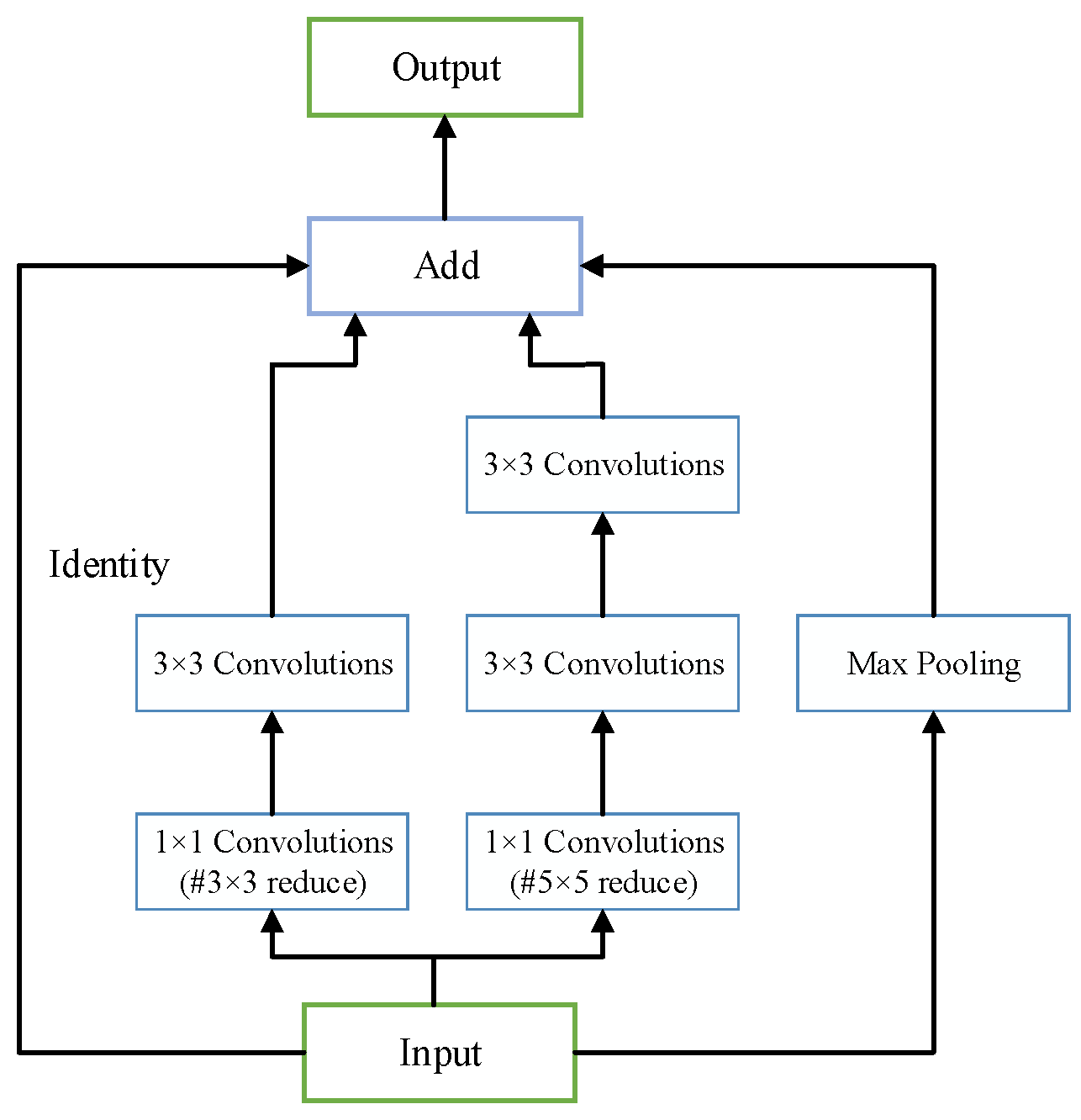
Based on the ideas of an Inception module [14,16] and a residual network [15], a new model architecture, the IRC module, was proposed, as shown in Figure 3.
The IRC module modified the original Inception structure by discarding the leftmost convolutional layer branch, whose convolutional kernel size was one. Following the idea of residuals, a shortcut was used to represent the identity of the input instead of the convolutional branch. The original four-branch output, concatenated in depth, was replaced by the sum of the four branches. That is, the feature vectors of the different branches were summed up according to their corresponding positions. This required not only the same size but also the same depth of the feature maps to be outputted from the four branches.
The IRC module structure differed from Inception–ResNet [18] in that it discarded the 1   ×   1 convolutional branch. The reason was that this convolutional branch was originally used to decrease the depth of the feature map, thus reducing the number of parameters of the network, which could not form an identity of the input. The IRC architecture required the output dimension to be the same as the input dimension, which eliminated the need for the branch to change the input dimension. Unlike the Inception–ResNet architecture, the IRC architecture did not discard the max pooling layer, which extracted the deep features of the SAR images with greater accuracy and improved the training efficiency.
A Batch Normalization (BN) layer was added before the activation function to perform the normalization operation for small batches during training. The BN layer can set a higher learning rate, reduce the training time, and solve the internal covariate shift phenomenon and degradation problems that exist in the network [15]. Dropout [24] was used with the fully connected layer to limit the overfitting ability of the model, slow down the model convergence, and improve the network generalization by randomly selecting the activation values of neurons to zero during the training process. Generally, the closer the dropout is to 0.5, the more accurate the performance; the closer to 0 or 1, the less accurate the performance. The SoftMax classifier was used at the output to normalize the model output values to between 0 and 1, classify them according to the magnitude of the probability values, calculate the model loss values using the cross-entropy loss function, and update the convolutional layer weight parameters by a back-propagation of errors.

4. Model Results and Analysis

In combination with the IRC module in Figure 3, the convolutional neural network model framework used in this experiment was built, as shown in Figure 4. The network first underwent three convolution layers to initially extract the image feature values, which were used as an input for the IRC module after a maximum pooling layer. A total of four large IRC modules were used, each containing two smaller IRC modules and a maximum pooling layer. Finally, after two fully connected layers, the final results were outputted by a SoftMax classifier.

4.1. Training Parameters Settings

Pre-processing operations such as homogenization and normalization were performed on the constructed dataset to unify the SAR image format. The image size was scaled down from 512   ×   512 to 224   ×   224 in accordance with the literature [13,14,15] for more effective convolutional operations and the extraction of image features. The training dataset was horizontally flipped and rotated by 10 ; other data enhancement techniques [25] were used to further expand the training set, reduce the overfitting of the model, and obtain more effective classification results. The model was trained for a total of 100 epochs, and the image batch size was set to 64. The larger the batch size, the more accurate the model training, but the longer the training time. The BN layer was added and its momentum size was set to 0.9. As the BN layer was added, there was no need to add bias terms to the convolution operation [16], which could have reduced the training parameters of the model. Dropout [24] was used in the fully connected layer of the model, with the parameter set to 0.5 to reduce model overfitting. The model parameters were optimized using the Adam optimizer with the learning rate set to 0.0001. There were 6,482,917 model training parameters.

4.2. Comparison of the Results and an Analysis of Different CNN Models

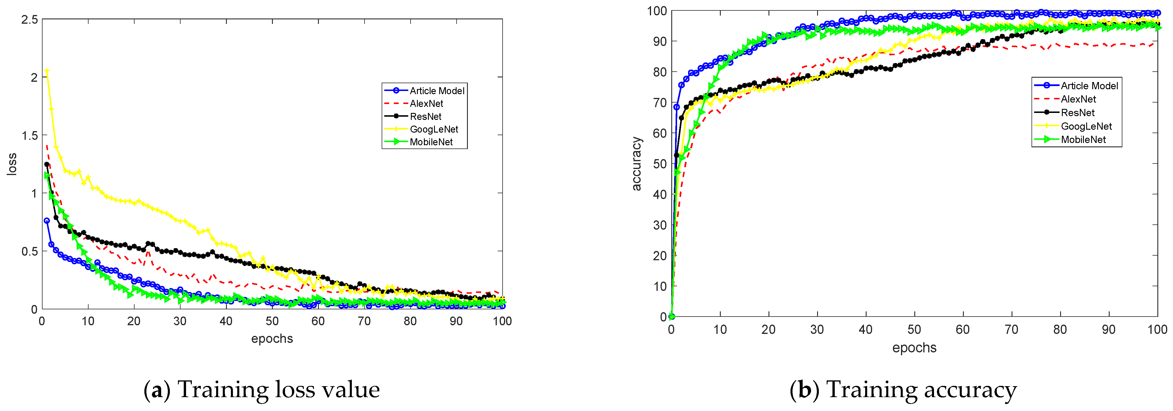
The training results of the model and the comparison results with the training of the other four classical models are shown in Figure 5. The paper model converged at the 50th epoch; the curve fluctuated less and stabilized in the subsequent iteration cycles. The model accuracy reached 98.79% and the model loss value was approximately 0.0351.
Compared with other classical algorithms, the convergence speed of the model was second only to MobileNet-V3, which reaches stability at the 30th epoch. The slightly slower convergence may have been because MobileNet-V3 combines the depth wise separable convolutions of previous versions, the inverted residual with the linear bottleneck, and the lightweight attention model of MnasNet’s squeeze and excitation structures. These structures allow a network to converge at a faster rate, but this also increases the training time to an extent. Among the five algorithms, our paper model had the highest classification accuracy and the lowest semantic loss value. As the IRC module could increase the depth of the network, it allowed the model to extract SAR image features at a deeper level; thus, it could reduce model overfitting and improve the training accuracy of the model. To exclude training serendipity and further verify the effectiveness of the model, the model was repeated several times; the average accuracy of the model was 98.71%, with an average loss value of 0.0374.
Table 2 compares the accuracy and the loss values of a few of the models in this paper with the four classical models mentioned above and three recently improved models. As can be seen from the table, the accuracy of the network improvement model proposed in this paper has improved considerably compared with the remaining four classical network models such as AlexNet. Our model was improved on the basis of ResNet and GoogLeNet; the accuracy of classification is improved by approximately 3% and the loss value was only 0.0374, which was much smaller than the other four models. When comparing the model of this paper with other improved models, the classification accuracy also improved by approximately 1%, which verified the feasibility and effectiveness of the model.

4.3. CNN Model Evaluation

For a further analysis of the above results, the model training results were evaluated using the validation set images for the trained model architecture parameters with the evaluation metrics of recall, accuracy, and F1-score. The specific expressions for each metric are shown below [21]:
R e c a l l = T P T P + F N ,
P r e c i s i o n = T P T P + F P ,
F 1 - s c o r e = 2 × P r e × R e c P r e + R e c ,
where P and N denote positive and negative samples, respectively, and T and F indicate correct and incorrect classifications, respectively. The F1-score metric combines both recall and precision metrics, and it is mostly used when the precision and recall rates do not determine the merit of the model. The closer the values of the above metrics are to 1, the more accurate the model is. Notably, recall, precision, and F1-score were all evaluated for a particular category.
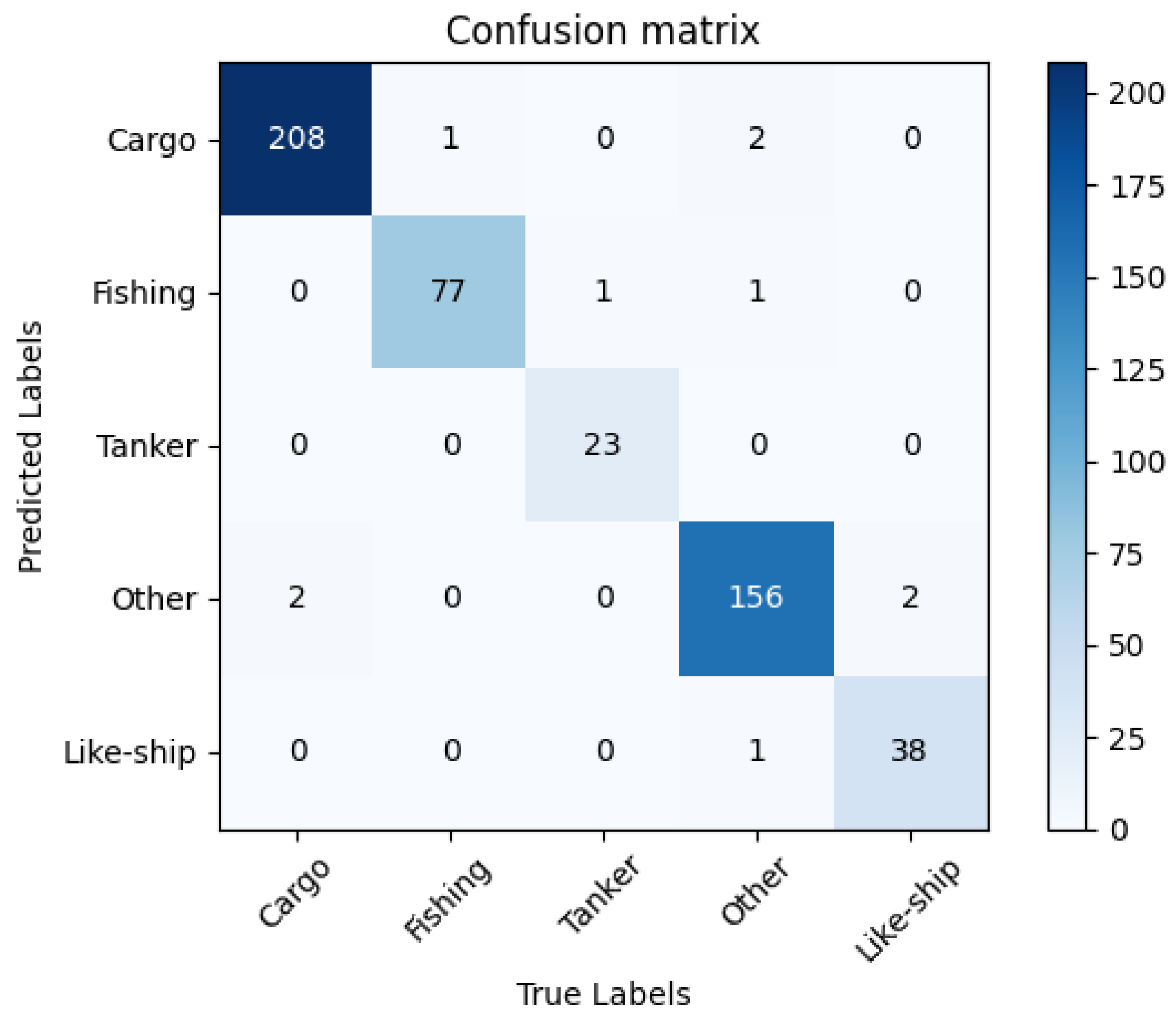
The model parameters after repeated training were saved, and the best model parameters with the highest accuracy were obtained for the predictive classification of the validation dataset. A confusion matrix of the model was obtained, as shown in Figure 6. Based on the results of the confusion matrix, three evaluation metrics were separately calculated according to the above equations. The evaluation results are shown in Table 3.
The evaluation results of the improved network model in this paper were higher than 95% for five different categories of image data, which indicated that the proposed network model had a higher classification accuracy. The robustness of the model was further improved due to the addition of the Like-Ship category. The Tanker category had the best evaluation result; the Cargo and Other categories had good evaluation results. Incorrect classifications were also mainly concentrated in these two categories because they had the largest amount of data. There were two main reasons for this situation. One was that these two categories had a larger amount of data compared with the other three categories, which could cause overfitting of the network model to an extent. The other reason was that these five categories, especially the Other category, contained multiple subcategories. The subcategories within the different large categories can exhibit similar image features, such as Utility Vessel in the Other category and Bulk Carrier in the Fishing category, thus causing errors in model predictions.

4.4. Discussion

The network model in this paper achieved the highest classification accuracy and the lowest semantic loss value in the high-resolution SAR ship dataset. This was mainly due to the deep feature extraction of the IRC module, combined with the ideas of classical network models to build a new model training network, i.e., the incorporation of the Inception module and residual structures to achieve identity mapping of the feature map.
There are many other factors that affect the classification performance of ships, such as the resolution of the image, the size of the ship, the wind speed of the ocean at the time of imaging, the state of the ocean, and the angle of incidence. In the literature [27], the detectability of the ship size, wind speed, and angle of incidence on ships has been verified by empirical models. The literature [11] points out that different preprocessing methods also have a significant impact on classification results, and emphasis is placed on proposing new chip acquisition methods to obtain more accurate features of a dataset. In this paper, we only considered the effects of network structure and network depth on classification accuracy; the effects of the above factors on SAR image features and ship classification results were not explored in detail. In future work, we will continue to analyze the effects of other factors on classification accuracy of SAR ship images. We will also continue to explore the impact of different network architectures on the classification accuracy. When the theory is mature, practice using real ports and other scenarios will also be considered.

5. Conclusions

The feature extraction and analysis of high-resolution SAR images is one of the common methods used in marine work such as ship management. With continuous breakthroughs in machinery, automation, and material technologies, the variety of ships is increasing. A deep-learning-based ship classification technique was proposed using the SAR image dataset. Our aims were to create a simpler and more efficient method to manage the classification of ships in the ocean and subsequently extend it to more complex working conditions for small-target identification tasks.
In SAR images, due to the influence of ship materials and structures, the SAR imaging angle, the ocean wind speed, and other factors, various ship types show distinctive image features under different situations. We used a CNN approach to deeply extract these features. Combining the ideas of a classical structure, an IRC module was proposed that could reduce the overfitting and degradation problems of the model. We changed the overall structure of the network, reduced the network parameters, and increased the network depth. The results showed that, compared with other classical CNN architectures, the classification accuracy of the model improved by approximately 3%, and the semantic loss value was minimized. It also sped up the convergence of the model and had more effective stability. Compared with other improved network results, the model accuracy improved by approximately 1% and the network structure was easy to implement. Thus, the proposed CNN classification algorithm efficiently identified ship images and achieved accurate classification results.

Author Contributions

Methodology, H.G.; software, L.R.; validation, H.G. and L.R.; formal analysis, H.G.; investigation, L.R.; resources, H.G.; writing—original draft preparation, L.R.; writing—review and editing, H.G.; visualization, L.R.; supervision, H.G.; project administration, H.G. All authors have read and agreed to the published version of the manuscript.

Funding

This research was funded by Natural Science Basic Research Plan in Shaanxi Province of China, grant number 2023-JC-QC-0714.

Data Availability Statement

All data that support the findings of this study are available from the corresponding author upon reasonable request.

Conflicts of Interest

The authors declare no conflict of interest.

References

  1. Chen, X.W. Research on Ship Classification Technology Based on Deep Learning. Ship Sci. Technol. 2019, 41, 142–144. [Google Scholar]
  2. Inggs, M.R.; Robinson, A.R. Neural approaches to ship target recognition. In Proceedings of the International Radar Conference, Alexandria, VA, USA, 8–11 May 1995. [Google Scholar]
  3. Musman, S.; Kerr, D.; Bachmann, C. Automatic Recognition of ISAR Ship Images. IEEE Trans. Aerosp. Electron. Syst. 1996, 32, 1392–1404. [Google Scholar] [CrossRef] [Green Version]
  4. Pastina, D.; Pastina, C. Multi-feature based automatic recognition of ship targets in ISAR images. In Proceedings of the 2008 IEEE Radar Conference, Rome, Italy, 26–30 May 2008. [Google Scholar]
  5. Jeon, H.K.; Jeon, C.S. Enhancement of Ship Type Classification from a Combination of CNN and KNN. Electronics 2021, 10, 1169. [Google Scholar] [CrossRef]
  6. Ren, Y.M.; Yang, J.; Guo, Z.Q.; Cao, H. Ship Classification Based on Attention Mechanism and Multi-Scale Convolutional Neural Network for Visible and Infrared Images. Electronics 2020, 9, 2022. [Google Scholar] [CrossRef]
  7. Suo, Z.; Suo, Y.; Chen, S.; Hu, Y. BoxPaste: An Effective Data Augmentation Method for SAR Ship Detection. Remote Sens. 2022, 14, 5761. [Google Scholar] [CrossRef]
  8. Zhang, Y.H.; Li, L.G. Application of Improved SqueezeNet in Ship Classification. Transducer Microsyst. Technol. 2022, 41, 150–152. [Google Scholar]
  9. Hou, X.Y.; Ao, W.; Song, Q.; Lai, J.; Wang, H.P.; Xu, F. FUSAR-Ship: Building a High Resolution SAR-AIS Matchup Dataset of Gaofen-3 for Ship Detection and Recognition. Sci. China 2020, 63, 40–58. [Google Scholar] [CrossRef] [Green Version]
  10. Ma, M.; Chen, J.; Liu, W.; Yang, W. Ship Classification and Detection Based on CNN Using GF-3 SAR Images. Remote Sens. 2018, 10, 2043. [Google Scholar] [CrossRef] [Green Version]
  11. Wang, Y.; Wang, C.; Zhang, H.; Dong, Y.B.; Wei, S.S. Automatic Ship Detection Based on RetinaNet Using Multi-Resolution Gaofen-3 Imagery. Remote Sens. 2019, 11, 531. [Google Scholar] [CrossRef] [Green Version]
  12. Alex, K.; Ilya, S.; Geoffrey, E.H. ImageNet Classification with Deep Convolutional Neural Networks. Commun. ACM 2017, 60, 84–90. [Google Scholar]
  13. Szegedy, C.; Liu, W.; Jia, Y.Q.; Sermanet, P.; Reed, S.; Anguelov, D.; Erhan, D.; Vanhoucke, V.; Rabinovich, A. Going Deeper with Convolutions. In Proceedings of the 2015 IEEE Conference on Computer Vision and Pattern Recognition (CVPR), Boston, MA, USA, 7–12 June 2015. [Google Scholar]
  14. Karen, S.; Andrew, Z. Very Deep Convolutional Networks for Large-Scale Image Recognition. In Proceedings of the ICLR, San Diego, CA, USA, 7–9 May 2015. [Google Scholar]
  15. He, K.M.; Zhang, X.Y.; Ren, S.Q.; Sun, J. Deep Residual Learning for Image Recognition. In Proceedings of the 2016 IEEE Conference on Computer Vision and Pattern Recognition (CVPR), Las Vegas, NV, USA, 27–30 June 2016. [Google Scholar]
  16. Ioffe, S.; Szegedy, C. Batch Normalization: Accelerating Deep Network Training by Reducing Internal Covariate Shift. In Proceedings of the 32nd International Conference on Machine Learning, Lille, France, 6–11 July 2015. [Google Scholar]
  17. Szegedy, C.; Vanhoucke, V.; Ioffe, S.; Shlens, J. Rethinking the Inception Architecture for Computer Vision. In Proceedings of the 2016 IEEE Conference on Computer Vision and Pattern Recognition (CVPR), Las Vegas, NV, USA, 27–30 June 2016. [Google Scholar]
  18. Szegedy, C.; Ioffe, S.; Vanhoucke, V.; Alemi, A.A. Inception-v4, Inception-ResNet and the Impact of Residual Connections on Learning. In Proceedings of the Thirty-First AAAI Conference on Artificial Intelligence (AAAI-17), San Francisco, CA, USA, 4–9 February 2017. [Google Scholar]
  19. Liu, Z.; Lin, Y.T.; Cao, Y.; Hu, H.; Wei, Y.X.; Zhang, Z.; Lin, S.; Guo, B.N. Swin Transformer: Hierarchical Vision Transformer using Shifted Windows. In Proceedings of the 2021 IEEE/CVF International Conference on Computer Vision (ICCV), Montreal, QC, Canada, 10–17 October 2021. [Google Scholar]
  20. Li, B.Z. Review of the Researches on Convolutional Neural Networks. Comput. Era 2021, 4, 8–12. [Google Scholar]
  21. Yadav, P.K.; Burks, T.; Frederick, Q.; Qin, J.W.; Kim, M.; Ritenour, M. Citrus Disease Detection Using Convolution Neural Network Generated Features and Softmax Classififier on Hyperspectral Image Data. Front. Plant Sci. 2022, 13, 1043712. [Google Scholar] [CrossRef] [PubMed]
  22. Zhang, Z.J. Improved Adam Optimizer for Deep Neural Networks. In Proceedings of the 2018 IEEE/ACM 26th International Symposium on Quality of Service (IWQoS), Banff, AB, Canada, 4–6 June 2018. [Google Scholar]
  23. Tang, S.H.; Teng, Z.S.; Sun, B.; Hu, Q.; Pan, X.F. Improved BP Neural Network with ADAM Optimizer and the Application of Dynamic Weighing. J. Electron. Meas. Instrum. 2021, 35, 127–135. [Google Scholar]
  24. Srivastava, N.; Hinton, G.; Alex, K.; Sutskever, I.; Salakhutdinov, R. Dropout: A Simple Way to Prevent Neural Networks from Overfitting. J. Mach. Learn. Res. 2014, 15, 1929–1958. [Google Scholar]
  25. Connor, S.; Taghi, M.K. A Survey of Image Data Augmentation for Deep Learning. J. Big Data 2019, 6, 60. [Google Scholar]
  26. Chen, Y. Research on Image Classification and Recognition in Ocean Going Ship Target Detection. Ship Sci. Technol. 2022, 44, 177–180. [Google Scholar]
  27. Tings, B.; Bentes, C.; Veloto, D.; Voinov, S. Modeling Ship Detectability Depending on TerraSAR-X-Derived Metocean Parameters. CEAS Space J. 2019, 11, 81–94. [Google Scholar] [CrossRef] [Green Version]
Figure 1. The specific details of the FUSAR-Ship dataset. The Ship category contains 15 major ship categories and 98 subcategories, with 5242 SAR images. The Like-Ship category contains bridges, lands, sea clutter waves, etc., with 427 SAR images. The amount of SAR image data varies for each category, and more than half of the categories have fewer than 100 SAR image data.
Remotesensing 15 02917 g001
Figure 2. Example of FUSAR-Ship dataset images. Different vessel types exhibit different features on the SAR images.
Remotesensing 15 02917 g002
Figure 3. Inception–Residual Controller (IRC) model architecture diagram. There were four branches in total; the left one represents the shortcut, the right one represents maximum pooling, and the middle two branches represents the convolutional branches. The symbol # indicates that the layer performs dimensionality reduction on the input, and the subsequent number indicates the size of the convolution kernel for the next layer of convolution.
Remotesensing 15 02917 g003
Figure 4. CNN model framework. In the figure, Input indicates the model input, Conv indicates convolution, IRC indicates the proposed module, Dense is the fully connected layer, and Output is the model output. The blue squares denote the convolutional layer, and the white squares denote the pooling layer, except for the final square, which is the global pooling value, all others show maximum pooling. The width, height, and depth of the feature map are shown in parentheses.
Remotesensing 15 02917 g004
Figure 5. Comparison graph of model training results. The left figure shows the comparison of the loss value of the model, and the right figure shows the comparison of the classification accuracy of the model. The figure shows that the model in this paper had a fast convergence rate, the highest model classification accuracy, and the smallest model loss value.
Remotesensing 15 02917 g005
Figure 6. Confusion Matrix. The diagonal line indicates the correct classification, i.e., TP. For each category, the vertical direction of the True Labels indicates FN and the horizontal orientation of the True Labels indicates FP. The remaining part indicates TN.
Remotesensing 15 02917 g006
Table 1. Data sheet.
Data CategoryTraining SetValidation SetTotal
Cargo19032112114
Fishing71178789
Tanker22424248
Other14471601607
Like-Ship38740427
Total46725135185
Table 2. Accuracy comparison table for eight models.
ModelAccuracy (%)Loss
AlexNet88.630.1443
GoogLeNet95.840.0912
ResNet95.490.1161
MobileNet95.280.0528
Zhang [8]96.61----
Wang [11]97.56----
Chen [26]97.72----
Article Model98.710.0374
Table 3. Summary of evaluation indicator results.
Evaluation IndicatorsPrecision (%)Recall (%)F1-Score (%)
Cargo98.5899.0598.81
Fishing97.4798.7298.09
Tanker10095.8397.87
Other97.5097.5097.50
Like-Ship97.4495.0096.20
Disclaimer/Publisher’s Note: The statements, opinions and data contained in all publications are solely those of the individual author(s) and contributor(s) and not of MDPI and/or the editor(s). MDPI and/or the editor(s) disclaim responsibility for any injury to people or property resulting from any ideas, methods, instructions or products referred to in the content.