Article

A Multi-Variable Sentinel-2 Random Forest Machine Learning Model Approach to Predicting Perennial Ryegrass Biomass in Commercial Dairy Farms in Southeast Australia

by
Elizabeth M. Morse-McNabb
1,2,*,
Md Farhad Hasan
3 and
Senani Karunaratne
1,4
1
Agriculture Victoria Research, Ellinbank Smart Farm, 1301 Hazeldean Road, Ellinbank, VIC 3821, Australia
2
Centre for Agricultural Innovation, Faculty of Science, School of Agriculture, Food and Ecosystem Sciences, The University of Melbourne, Grattan Street, Parkville, VIC 3010, Australia
3
Agriculture Victoria Research, AgriBio La Trobe University, 5 Ring Road, Bundoora, VIC 3083, Australia
4
CSIRO Agriculture and Food, Black Mountain Science and Innovation Park, Clunies Ross Street, Canberra, ACT 2601, Australia
*
Author to whom correspondence should be addressed.
Remote Sens. 2023, 15(11), 2915; https://doi.org/10.3390/rs15112915
Submission received: 9 May 2023 / Revised: 27 May 2023 / Accepted: 29 May 2023 / Published: 2 June 2023
(This article belongs to the Section Remote Sensing in Agriculture and Vegetation)

Abstract

:
One of the most valuable and nutritionally essential agricultural commodities worldwide is milk. The European Union and New Zealand are the second- and third-largest exporting regions of milk products and rely heavily on pasture-based production systems. They are comparable to the Australian systems investigated in this study. With projections of herd decline, increased milk yield must be obtained from a combination of animal genetics and feed efficiencies. Accurate pasture biomass estimation across all seasons will improve feed efficiency and increase the productivity of dairy farms; however, the existing time-consuming and manual methods of pasture measurement limit improvements to utilisation. In this study, Sentinel-2 (S2) band and spectral index (SI) information were coupled with the broad season and management-derived datasets using a Random Forest (RF) machine learning (ML) framework to develop a perennial ryegrass (PRG) biomass prediction model accurate to +/−500 kg DM/ha, and that could predict pasture yield above 3000 kg DM/ha. Measurements of PRG biomass were taken from 11 working dairy farms across southeastern Australia over 2019–2021. Of the 68 possible variables investigated, multiple simulations identified 12 S2 bands and 9 SI, management and season as the most important variables, where Short-Wave Infrared (SWIR) bands were the most influential in predicting pasture biomass above 4000 kg DM/ha. Conditional Latin Hypercube Sampling (cLHS) was used to split the dataset into 80% and 20% for model calibration and internal validation in addition to an entirely independent validation dataset. The combined internal model validation showed R2 = 0.90, LCCC = 0.72, RMSE = 439.49 kg DM/ha, NRMSE = 15.08, and the combined independent validation had R2 = 0.88, LCCC = 0.68, RMSE = 457.05 kg DM/ha, NRMSE = 19.83. The key findings of this study indicated that the data obtained from the S2 bands and SI were appropriate for making accurate estimations of PRG biomass. Furthermore, including SWIR bands significantly improved the model. Finally, by utilising an RF ML model, a single ‘global’ model can automate PRG biomass prediction with high accuracy across extensive regions of all seasons and types of farm management.

1. Introduction

Dairy farms in Australia are largely grazing-based systems (almost 96%), utilising pasture as a nutrient-dense and cheap feed source for dairy animals [1,2]. This precious resource can be efficiently managed if measured, but in busy farming systems such as dairy, it is difficult to observe the whole farm all the time adequately using traditional on-farm pasture biomass measuring approaches. Fulkerson et al. [3] found that feed allocation for cows can vary by up to 50% from intake requirements per day. Therefore, pasture allocation and utilisation should be carefully monitored [4] to avoid high pasture availability leading to concentrate wastage or low pasture availability resulting in underfed cows. The efficient utilisation of high-quality farm-grown biomass is one of the critical attributes of a cost-effective pasture-based dairy farming system [5,6]. A robust and accurate method for estimating and mapping pasture biomass variation across whole farms and within paddocks is essential for sustainable dairy farm productivity in Australia and other regions dependent on pasture-based systems.
The challenge in estimating pasture biomass in the dairy industry is four-fold. Firstly, due to the regional differences in climate and access to irrigation, continuous pasture biomass prediction needs to consider a range of seasons simultaneously. Secondly, the biomass volume produced during the peak growth period (in any season) over very short intervals (~30 days) can quickly exceed 3000 kg DM/ha (dry matter per hectare). Thirdly, the paddocks can be as small as one hectare, which impacts measurement resolution. Finally, the grazing or harvesting frequency in dairy farming requires frequent observations to provide helpful information for supporting farm management and decision-making processes.
Many conventional and modern tools already provide pasture biomass prediction at the paddock scale. However, these tools are labour-intensive or inaccurate and rarely provide total farm views. One of the most basic and labour-intensive tools, the rising plate meter (RPM), uses a plate to measure compressed pasture height [7]. The process is tedious and can be time-consuming, particularly for large farms. In addition, for robust data collection, many individual measurements are required per paddock to provide a single paddock average; therefore, it does not comprehensively represent the spatial variability of the pasture [8]. On the other hand, there are a growing number of handheld sensors [9] or vehicle-mounted sensors (for example, multispectral sensors and ultrasonic sensors) [10] that enable semi-automatic field data collection. Although handheld and vehicle-mounted sensors are non-destructive methods, they still require time and access to traverse the pasture and may inadvertently damage the pasture or soil. Unmanned aerial vehicle (UAV) mounted sensors are becoming increasingly prevalent in agricultural settings [11,12]. However, these can only capture part of the farm in one day and require significant investment in equipment, sensors, software, and computational resources (i.e., automated analysis frameworks) to produce pasture biomass estimates.
Satellite remote sensing of aboveground biomass has been demonstrated for 50 years [13]. Recent advances in multispectral satellite sensors and constellation suites theoretically enable the regular measurement of pasture biomass and can automatically provide data over large areas, including regular revisit times. Many examples of spatio-temporal observation of biophysical characteristics of vegetation, such as biomass and leaf area index (LAI), were evident in the literature, including forests [14,15,16], crops [17,18,19], land cover [20,21,22], and certain forages [23]. Spatio-temporal observation has also been a popular choice for pasture biomass estimation [24,25,26]. However, many published studies did not focus on highly managed environments such as dairy farm systems or extend across large regions or periods [27]. Early studies focusing on dairy farming systems showed promising evidence that satellite platforms could estimate pasture growth and fertiliser needs that match the farm-scale requirement, even when using coarse-resolution sensors [28,29]. Furthermore, Edirisinghe et al. [30,31] showed that with improved satellite-based sensors and well-matched sampling strategies, it was possible to predict pasture biomass at the paddock scale on annual pastures in Western Australia and perennial pastures in Waikato, New Zealand.
Sentinel-2A and Sentinel-2B (S2) satellites, launched by the European Space Agency (ESA), are now popularly favoured for biomass mapping due to the five-day revisit cycle (at the equator) and 12 bands with resolutions ranging from 10 m to 60 m [25,32,33,34]. An additional benefit is that the data is freely available. The short revisit time and large swath width (290 km) theoretically enable regular measurement subject to cloud cover. One of the advantages of using S2 imagery is the addition of SWIR bands. The pixel resolution is also adequate for smaller dairy farm paddock areas.
An extensive array of studies has demonstrated processing options for multispectral sensor bands, such as single bands [35], commonly reported spectral indices, linear spectral unmixing [26], spectral mixture analysis [36], and using the principles of radiation use efficiency [37], and physically-based radiative transfer modelling [38]. Vegetation indices are the most common approach, with the normalised difference vegetation index (NDVI) being the most widely used and reported over the last 50 years and commonly used as a reference index on which to gauge improvement [26,39,40]. Although NDVI has been proven to be an excellent predictor of biomass in many studies, the challenges of fast-growing high-volume wet canopies, such as those found in dairy pastures, suggest the investigation of a suite of spectral indices (SI). Numata et al. [36] found better correlations with fresh weight than dry weight using two indices that use SWIR bands. SWIR bands have been found to improve the correlations between the measured and predicted dry weight due to sensitivity to leaf water concentration at high biomass (>3000 kg DM/ha). Biomass above 3000 kg DM/ha is a level that commonly exceeds a Leaf Area Index (LAI) greater than 3. LAI > 3 is known to saturate common vegetation indices such as the Normalised Difference Vegetation Index (NDVI) [41]. Broge and Leblanc [42] demonstrated that the effectiveness of SI depends not just on the bandwidth or combination but also on the target’s range and environmental factors such as soil classification and colour variations in the soil in both dry and wet conditions and moisture present in the air that affect that range.
With the ever-increasing data from modern satellite sensors, selecting a proper empirical modelling framework is essential in landscape research. The linear regression analysis approach has been favoured for data analysis, particularly for satellite-based work [31,32,43]. Guerini Filho et al. [32] considered multiple linear regression analyses for natural grassland biomass estimation by SI and obtained a coefficient of determination (R2) less than 0.70. Although the accuracies were satisfactory, the major disadvantage of the approach is the site-dependent research and inability to capture the complex non-linear patterns found in the data. Therefore, the algorithm will likely have greater errors for the diverse pasture types in dairy management systems due to the design of the study presented by Guerini Filho et al. [32].
Machine Learning (ML) algorithms have efficiently handled large datasets, particularly the ones with non-linear patterns. Recent progress in digital agriculture has also triggered the necessity of state-of-the-art ML approaches to increase the efficiency of model prediction with further automation [44]. ML has been used in agricultural applications, particularly for pasture biomass prediction [25]. However, there is no universal measure of ML suitability [45]. Among different ML techniques, non-parametric supervised classifiers such as support vector machine (SVM) [46], artificial neural networks (ANN) [47,48], k-nearest neighbor (kNN) [49], classification and regression tree (CART), and supervised techniques such as Random Forest (RF) have been widely used for predicting biomass based on satellite images [50,51].
The significant objectives of this study are summarised as the following:
  • Combine S2 and ML modelling approaches to predict perennial ryegrass biomass across a range of regions and seasons with an accuracy of +/−500 kg DM/ha.
  • Provide technical evidence that utilising SWIR bands can improve the ability to predict pasture yields above 3000 kg DM/ha and, therefore, enable measurements of high-yielding pastures at any stage in the growth cycle in irrigated and dryland farm management systems.
  • Examine the pasture biomass prediction model quality through a fusion of S2 sensor-derived datasets and broad management and seasonal datasets.
  • Show that it is possible to predict pasture biomass across large regions and growing seasons on commercial dairy farms with one ‘global’ model with an extensive ground sampling campaign and the use of numerous bands and SI of the S2 sensor and the ML modelling framework.

2. Materials and Methods

2.1. Study Site Location, Soil, and Climate and Sampling Design

A total of 11 commercial dairy farms were part of this study. Seven farms were intensively sampled and contributed to the calibration and validation dataset. The remaining farms were sampled once to obtain fully independent validation data. Four farms were in the Northern Irrigation Region of Victoria, two in the Macalister Irrigation District in far eastern Victoria, two in West Gippsland, two in the southwest of Victoria, and one in the southeast of South Australia, as illustrated in Figure 1. Four of the eleven farms were dryland farms, and the remaining properties applied irrigation water to some or all of the grazed pastures using flood irrigation or overhead sprinklers. Farm sizes ranged from 72 to 970 ha.
The average paddock size per farm ranged from 1.2 to 15.7 ha. The Northern Irrigation District farms have the lowest average annual rainfall and the highest temperatures, while the West Gippsland farms have the highest average annual rainfall and a milder temperature range (Table 1). Key land management options and soil characteristics across the farms are also summarised in Table 1.
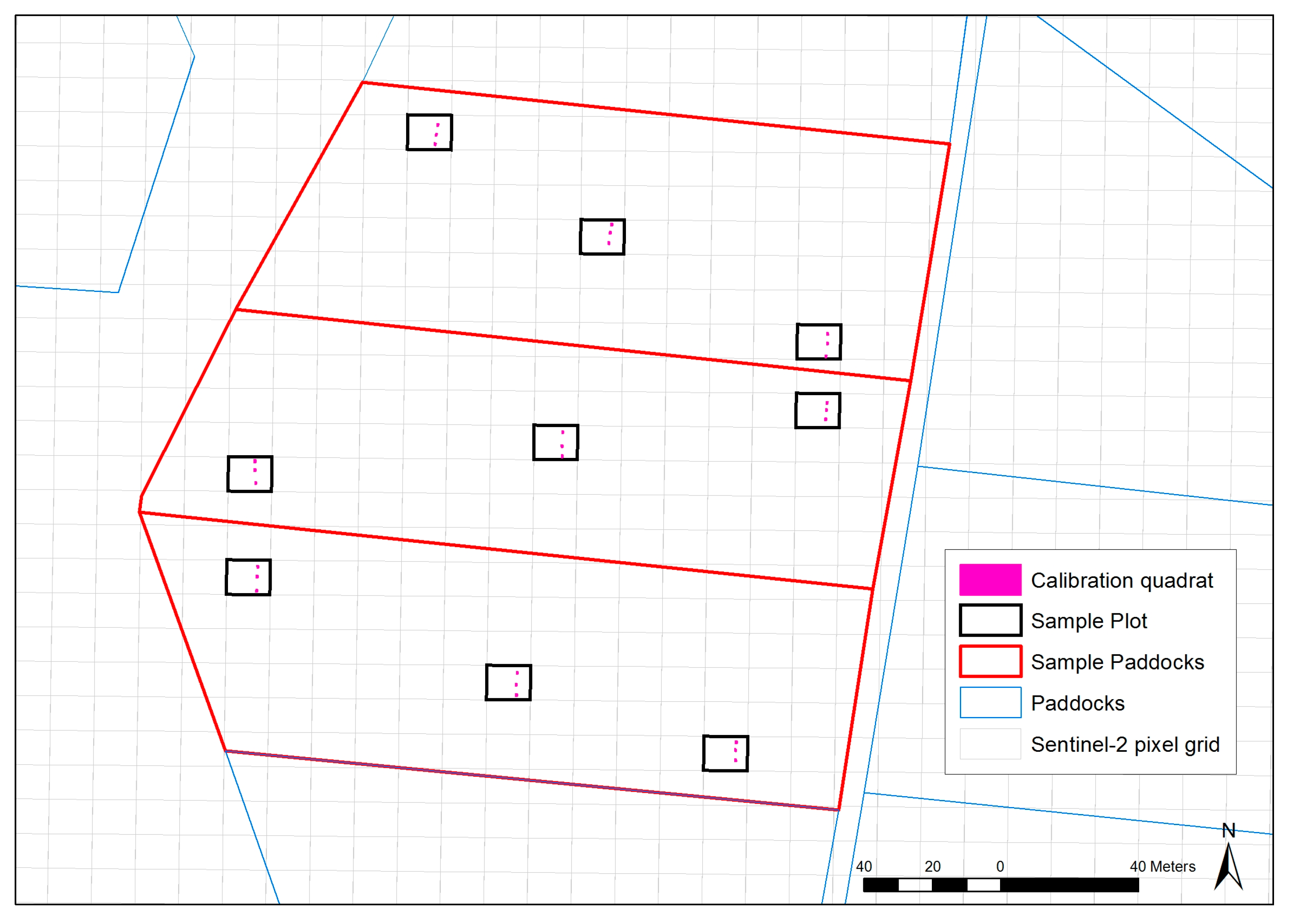
Two paddocks on each of the seven calibration farms were measured regularly (weekly to monthly intervals). On each visit, three destructive samples were removed from at least five predetermined 10 × 10 m areas across the two paddocks. The 10 × 10 m areas were based on the S2 pixel grid to enable direct comparison of field data and image observations, as shown in Figure 2. The sampling procedure was replicated on the four independent validation farms. Two paddocks were sampled on each of these farms; however, these farms were sampled only once.

2.2. Ground Data Collection

Field data collection across all eleven farms was consistently applied using the following procedures. All field data collection and in-field navigation were performed using Emlid RTK GPS units with a spatial precision of +/−2 cm. The destructive sample areas varied between 70 × 35 cm and 64 × 31 cm quadrats. Within these quadrats, observations of plant leaf stage, botanical composition, and three measurements of height (ruler, rising plate meter, and sonar) were taken before sampling and recorded in the field using the ESRI Collector field application [54]. The pasture was cut to ground level, bagged, weighed fresh, washed to remove soil and debris, and then oven-dried at 100 °C for 24 h or until a constant weight was recorded. In addition, a vehicle-mounted wide-angle ultrasonic sensor and a UAV-mounted multispectral camera were simultaneously used during data collection, with results published separately [55,56,57]. In the previous works, while different sensors and numerical techniques were implemented, the focus remained on the prediction of pasture yield and nutritive characteristics with similar sample pre-processing approaches. The work of Karunaratne et al. [55] focused on UAV-based empirical numerical modelling approaches by considering Structure from Motion only (SfM), vegetation indices (VI) only, and finally, SfM + VI combination. Meanwhile, Lawson et al. [56] presented global ultrasonic (vehicle-mounted) and RPM models using linear mixed models to predict pasture biomass, and Thomson et al. [57] compared different modelling approaches using hyperspectral datasets to predict pasture biomass and nutritive characteristics.
Data collected in the field was later downloaded from ESRI Collector via ArcGIS Online [58] (AGOL) and saved to an ESRI File Geodatabase. Polygon data were transformed from the WGS84 projection to the UTM zone appropriate for each farm to match the S2 data.

2.3. Satellite Data Collection

This study was aligned with a broader study where the aim was to test a variety of sensors. One study design and collection protocol were utilised for multiple sensors to reduce the operational cost across the programme. Since ground data collection timing depended on appropriate UAV flying conditions (wind speed and rain) and rarely coincided with satellite overpass dates, a process was developed to select the most appropriate S2 image for each collection date. This process considered images before and after field data collection, the time of year, location, grazing, and the number of days between the field data collection and image acquisition.
Intensively managed dairy pastures are grazed frequently. However, grazing times recorded by the farmer were not always available or accurate. Therefore, a method was developed to identify the timing of field measurement relative to grazing, which enabled the appropriate selection of a satellite image. The image selection technique calculated the measured mean above-ground biomass (kg DM/ha) for each paddock on each collection day. These individual collection averages were combined to create summary statistics (minimum, maximum, mean, and standard deviation) for each paddock over the complete time series. If the mean biomass on the collection day was less than the minimum plus the standard deviation of the total paddock collection biomass, then grazing had recently occurred. As grazing may have occurred the previous day, it was important to use an image acquired after the ground collection date. On the contrary, if the mean biomass on the day of collection was greater than the maximum minus the standard deviation of the total paddock collection, then it was likely that grazing would occur after the day of ground collection. Therefore, an image acquired before the ground collection date was chosen (Figure 3). This process was only used for the calibration and internal validation dataset. Independent validation data were unique; therefore, the closest image to the collection date was chosen. Trampling the area within and around the pixel may be possible in 34% of images acquired after the ground collection date; however, this was not considered a parameter in the image selection approach.
Pasture accumulation rates differ broadly between regions and months and depend on farm management. Based on the reported accumulation rates from Figures 8, 11, 12, and 13 of Doyle et al. [59], a maximum number of days of lag per month was established to limit the potential growth differential between measurement and overpass of less than 200 kg DM/ha. The current study extended no image lag date beyond five days. Currently, no average monthly pasture growth rates are reported for irrigated dairy pastures in southeast South Australia. The southeast South Australia site was a summer irrigated system, as were the Northern Irrigation Region Sites and the Macalister Irrigation Region sites. Therefore, the shortest lag rule from those two sites was applied as a precautionary approach.
Data were collected from May 2019 to July 2021. A total of 200 paddock data collection dates and 100 S2 image datasets, with less than 15% cloud, were available across the seven calibration farms between May 2019 and March 2020. Of the available calibration data, 75 paddock collection datasets matched 40 S2 images; however, on closer inspection, the cloud affected eight images. Therefore, the final calibration data collection included 45 paddock datasets and 30 S2 images. Using the same approach for all data available from April 2020 to July 2021, a final validation collection included 16 paddock datasets and eight S2 images. Figure 4 overlays the image acquisition and ground collection dates for the calibration and validation dataset, separated by farm, for a comprehensive understanding. The reduction in data availability from March 2020 to April 2021 was due to COVID-19 lockdowns restricting farm access.

2.4. Data Processing—Satellite Spectral Index Calculations and Stacking with Bands

Level 2A, Sentinel-2A, and 2B images with less than 15% cloud were downloaded from the Sentinel Australasia Regional Access (SARA) website (https://copernicus.nci.org.au/sara.client/#/home, accessed on 15 June 2020). Image data processing occurred in ENVI®+IDL version 5.6 [60]. Each dataset was spatially subsampled to an area of interest (AOI) that included the whole farm (not just the paddocks sampled), each band resampled to 10 m resolution and stacked in a 12-band TIF file. Information on the original S2 bands has been included in Table 2 (rows 55 to 66). The “GainOffset” function was used with offset value for all bands set to 0.0001, and a high (1.0) and low (0.0) clip was applied. Fifty-four spectral indices (SI) were then calculated for each image using an ENVI®+IDL model and stacked into a 54-band TIF file. All SI are listed in Table 2 (rows one to 54). The initial 54 index selection was made from an extensive list curated from a literature review to identify those indices that could be calculated using S2 bands. Each SI was reviewed considering the bandwidths and centre wavelength of the S2 sensors rather than the traditional band designation or the original S2 band spatial resolution. Consideration was also given to the sensor initially used to develop the index. Each index calculation was tested in ENVI to ensure the notation was calculated as defined in the original reference. Simple ratios or difference indices were calculated using all available band combinations to test the sensitivity of the full array of bands available on the S2 sensors.

2.5. Data Merging

Due to the precise locational attribution of the in-field data collection, it was possible to combine field measurements with the satellite observations into one dataset. Each ground data collection dataset with a matching S2 image was converted to a point layer using the ‘Feature to Point’ tool in ESRI ArcMap 10.8 [91], and a unique S2 pixel identifier was added to generate summary statistics and other analyses at pixel scale as required. Pixel-level information from the 12-band and 54-SI stack were spatially joined to the ground data point layer using the ‘Extract Multi values to points’ tool in ESRI ArcMap 10.8 [91]. All individual datasets were stacked using the R programming language for analysis [92]. The R computation was conducted on a Windows® 10 operating system. The computer had a processor of 11th Gen Intel® CoreTM [email protected] 2.61 GHz processor with 64 GB RAM. The ML was run through the NVIDIA® RTX A3000 GPU to accelerate processing and improve numerical efficiency.

2.6. Pre-Processing and Development of Machine Learning Framework

Additional categorical variables were added to the dataset prior to modelling. As the season is an integral component of biomass modelling, the data were categorised into five seasonal periods consistent with the Australian forage value index [65,93]. The seasons were winter (June, July), early spring (August, September), late spring (October, November), summer (December, January, February), and autumn (March, April, May). In addition, information on regions and types of management (dryland or irrigated) was included (Table 1).
An ML approach was used to accommodate the high-dimensional datasets characterised by multi-collinearity among the dependent variables. The RF model was chosen among different ML approaches as it is an efficient technique for analysing linear and non-linear relationships [44]. Furthermore, RF is an ensemble, non-parametric, supervised approach that is widely applied in agricultural applications [94,95,96] and, therefore, considered appropriate to predict pasture biomass. RF models require additional functions to increase the efficiency and reliability of predictions, such as performing variable importance (VI) to optimise the feature space [44,97,98,99], presenting a correlation matrix to observe the relationships among the high dimensional datasets [100], and the detection of outliers [101], to name a few. In addition, several statistical interpretations and analyses, along with the data preparation, were performed to improve model performance, and these have been described in the following sections.

2.6.1. Shapiro–Wilk Test

In ML algorithms, outliers can deceive the sample training process, leading to increased training times and less accurate models [102]. Therefore, it was essential to conduct a detection check to identify outliers and normal distribution. The Shapiro–Wilk (SW) test was considered in this study with both calibration and validation datasets to test the null hypothesis, normality, and the detection of outliers due to its proven capability in digital agriculture, mainly when dealing with multivariate datasets [103]. The null hypothesis means that no direct relationship exists between the two variables being studied. A p-value, also known as the probability value, is an important parameter that is mostly observed to accept or reject a null hypothesis. Generally, a lower p-value refers to statistical significance and if the null hypothesis is rejected. In the present study, p < 0.05 was assigned to determine statistical significance. The calculation of the SW normality test was denoted by W (0 ≤ W ≤ 1), which shows how efficiently the ordered and standardised sample quantiles fit the standard normal quantiles, with 1 demonstrating a perfect match [102]. In the present study, W = 0.9596 and W = 0.9571 were obtained for internal and independent model validations, respectively, along with p < 0.05. Therefore, it improves confidence in the development of the model.

2.6.2. Conditional Latin Hypercube Sampling

Conditional Latin Hypercube sampling (cLHS) can be used for the spatial splitting of datasets for model calibration and internal validation [104,105,106] as ancillary variables occupy a hypercube in the feature, attribute, or variable space. The feature space can be sampled instead of sampling the whole geographical space. However, planning a sampling methodology that can select the sampling locations covering the hypercube of the feature space is a complicated task. Therefore, a widely used alternative is to consider cLHS, which is non-parametric, and additional conditions can be considered for model optimisations based on input features [105].
The obtained data was split into calibration and validation datasets (80% [n = 171] and 20% [n = 43]) using the cLHS algorithm. The library package “clhs” was used to perform the split [105]. The evolution of the objective function for the number of iterations was monitored to observe stability. The algorithm identifies the points that can represent a Latin hypercube through a random data sampling procedure. The dataset for cLHS was subjected to 2500 iterations to reach a steady state of the objective function. Subsequently, cLHS was used as an objective function for data splitting before calibration and internal validation of the RF ML algorithm.

2.6.3. Variable Importance Section through Boruta Algorithm

The RF approach is efficient but could be time-consuming for application across large spatial extents. Selecting variable importance (VI) is a standard practice in ML modelling to reduce the number of input variables. At the same time, this process allows the model to emphasise the variables which are more influential in predicting the output. Since input variables cannot be reduced or eliminated arbitrarily, standard algorithms are implemented into ML models to perform the feature selection task. While there is no universal yardstick of the most accurate algorithm to perform this task, the Boruta algorithm is popular, particularly for remote sensing ML modelling [44,107,108,109]. The Boruta algorithm is an ensemble technique and was considered in the ML approach to increase RF efficiency by reducing the number of variables. The library package “Boruta” was employed in the prediction model to perform feature selection by means of variable importance (VI) [109]. Therefore, Boruta ensures that the RF model is built based on only relevant and essential features with minimised data dimensionality.
The original variable list comprised 12 original S2 bands and 54 SI totalling 66 bands and indices (Table 2). In addition, season and management were included in the model as categorical variables. Therefore, a total of 68 input variables were considered initially before the final model development. Multiple Boruta algorithms were performed to identify the most influential bands and SI to reduce the number of variables. The best 21 bands consisting of 12 original bands and 9 SI were unbiasedly selected, as shown in Table 2 and as described in Section 2.7. Season and management were also found to be important through the feature selection approach. Therefore, the model was developed with season and management totalling 23 input variables as selected by Boruta. Boruta considered all the candidate features (original bands and SI, season, and management) to predict pasture biomass and randomly designed shadow versions of each feature. The maximum number of iterations was varied to ensure that all essential attributes were identified and the convergence state was monitored. Boruta runs were based on iterations written as a function called “maxRuns” in R, indicating the maximum number of iterations. In the current RF model, maxRuns = 1500 was found to be adequate for identifying all important variables since the VI selection decision was reached within 1500 iterations. The RF model was optimised once all requirements were fulfilled.

2.6.4. Random Forest Modelling

In this research, the RF model was performed in the R statistical programming environment, and the “ranger” package was used to create the model. The “ranger” package is a fast implementation of RF modelling and is specifically well-suited for analysing high-dimensional data [110,111]. Furthermore, this RF model was simple to implement, and in the current study, two key model parameters were needed to define: Ntree and mtry [110], along with additional associates to ensure smooth execution. The following briefly discusses some of the important parametric values considered in the RF model:
RF model parameters: The primary objective of RF model parameter tuning is to find the optimal hyperparameters for the calibration dataset. While the default RF setting has been reported to be less tunable, specific tuning search strategies (such as grid search) have assisted in evaluating the discrete parameters for the out-of-bag performance [110]. One of the primary tools is the “train” function embedded with the “caret” package [112], which was used to evaluate the RF model parameter tuning and estimate the performance from the training set. Furthermore, “tuneGrid” and “trainControl” arguments were integrated into the coding environment to generate the parametric values of the candidates and modify the resampling (if required). Additionally, the “repeatedcv” argument was used to integrate the repeated K-fold cross-validation, where the argument repeats controlled the number of repetitions. A specific number maintains K in the argument; by default, it is 10.
  • Ntree: The parameter Ntree refers to the number of decision trees generated. As per the literature, the standard requirement to analyse remote sensing data, i.e., a default value of Ntree = 500 was used [44].
  • mtry: The parameter mtry denotes the number of variables to be selected and tested for the best split while growing trees. Lower mtry values have been attributed to stability enhancement, as it reduces the number of correlated trees [110]. Several tests were included before selecting mtry values, as advised by Probst et al. [110]. In the present model, mtry = 6 was found to be the best with reduced computational time.
In RF, the default splitting rule considers a selection of variables with many possible combinations. However, it has been reported that the default rule favours the selection of the variables with many splits and can overlook variables with fewer splits [110]. This type of variable bias decreases RF efficiency, so a modified approach has been considered in this study. In this study, the splitting rule was randomised per the technique described in Geurts and Wehenkel [113]. In addition, the “extratrees” feature was considered. The function “extratrees” adds additional components of randomness to the trees in RF modelling. However, it has been observed that such randomness substantially impacts VI ranking and may lead to RF being biased [110]. The “permutation” function of VI was integrated into the R code to ensure an impartial VI [114].
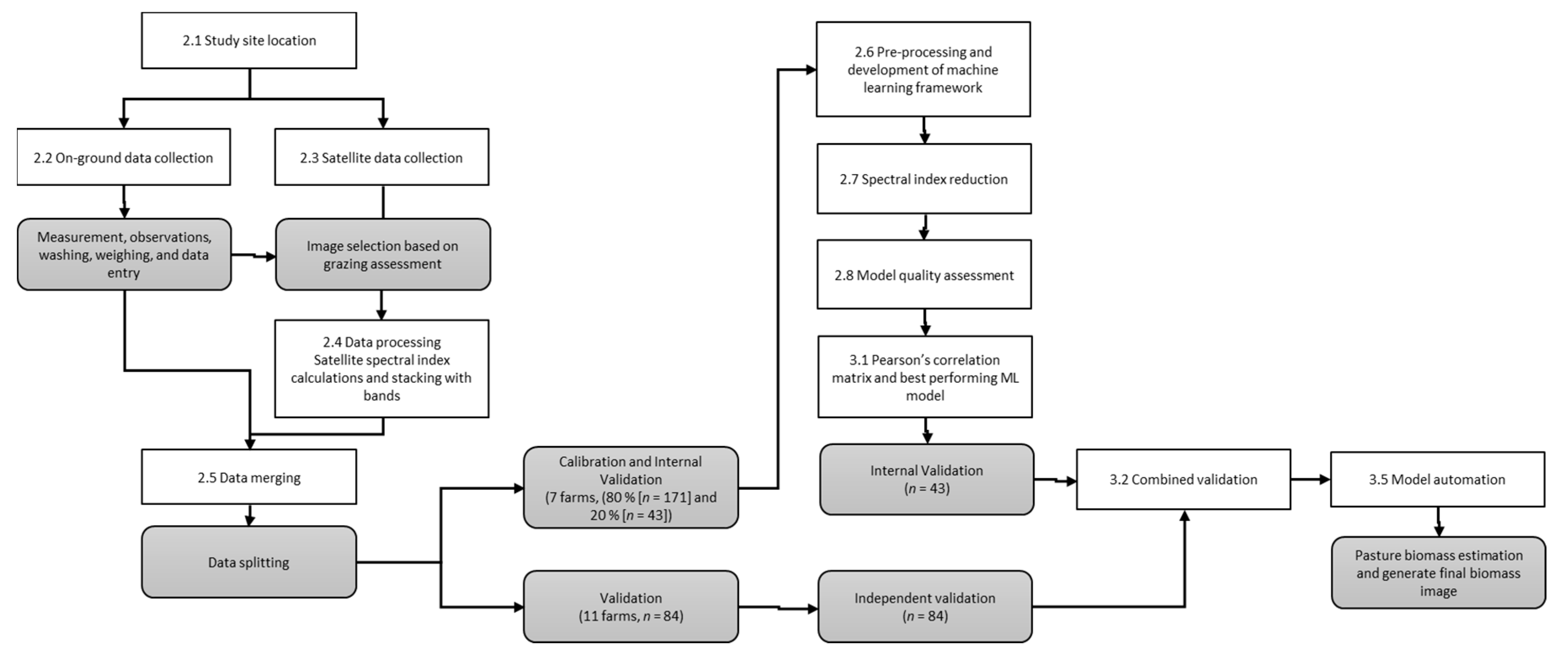
A complete flowchart outlining the data manipulation and analysis framework using the ML approach is shown in Figure 5.

2.7. Spectral Index Reduction

After several primary iterations for biomass estimation and prediction model development, 12 bands and 9 SI were selected using the outcomes of the Boruta algorithm. At least 12 iterations were made, and the results of the variable importance plot were collated. Row numbers 3, 14, 16, 22, 32, 34, 43, and 54 (column 1, Table 2) were always rejected. Row numbers 6, 8, 12, 13, 17, 19, 23, 36, and 48 (column 1, Table 2) were always important and used in the biomass estimation and prediction model. The remaining 37 spectral indices had variable results across model iterations. All were rejected at least once, and some up to eight times.

2.8. Model Quality Assessment

As mentioned earlier, the model prediction quality was tested through internal and fully independent validation. Different metrics were used to evaluate the model quality: (a) RMSE, which provides information on the model accuracy by calculating the differences between the predicted and observed values, (b) NRMSE, which is the calculated RMSE as a percentage of the measured mean of the data, (c) R2, and finally (d) Lin’s concordance correlation coefficient (LCCC).
The following equations describe the expression to determine the validation indices:
RMSE = i = 1 N Y Y i 2 N
where Y = measured pasture DM yield, Yi = predicted pasture DM yield, and N is the number of samples.
NRMSE = (RMSE/Mean measured pasture DM yield) × 100
LCCC depicts the variation of the predicted values from a unity line (1:1) [115]. LCCC is a measurement of the degree to which the predicted values adhere to the concordance line of slope 1.0 through the origin and an outcome of the product between the Pearson correlation coefficient and a bias factor reflecting the precision and accuracy. The bias factor information is achieved from mean and slope bias [115]. LCCC is defined as the following:
LCCC = 2 ρ σ x σ y σ x 2 + σ y 2 + μ x μ y 2
where mx and my are the measured and predicted pasture biomass means, respectively; sx2 and sy2 represent the variances of the measured and predicted pasture biomass. Meanwhile, r is the Pearson correlation coefficient between measured and predicted pasture biomass.

3. Results

3.1. Pearson Correlation Matrix and Best-Performing ML Model

Examining the relationships among the variables as well as the feature selection are two of the significant steps in the ML approach. Importantly, weaker relationships between the predictor and target variables affect the efficiency, prolong the training times of the samples, increase the computational complexities, and reduce the potential impact of significant parameters. Pearson’s correlation matrix is a popular method for demonstrating correlation among variables in ML. Each cell in the correlation matrix represents the correlation between two variables. The values are located between −1 and +1, with values closer to −1 and +1 indicating strong negative and positive correlations. A value closer to 0 demonstrates no connection between those variables. This study calculated Pearson’s correlation matrix to examine the correlation coefficient among the selected bands and spectral indices, as shown in Figure 6. In general, it was observed that all the bands considered to predict mean values of the dry matter showed good correlations, with Image Index Band_20 (B11 SWIR), Band_11 (B2 Blue), Band_19 (B9 Water vapour), and Band_21 (B12 SWIR) showing the strongest correlations. None of the bands exhibited a null value (0) to predict dry matter.

3.2. Combined Validation

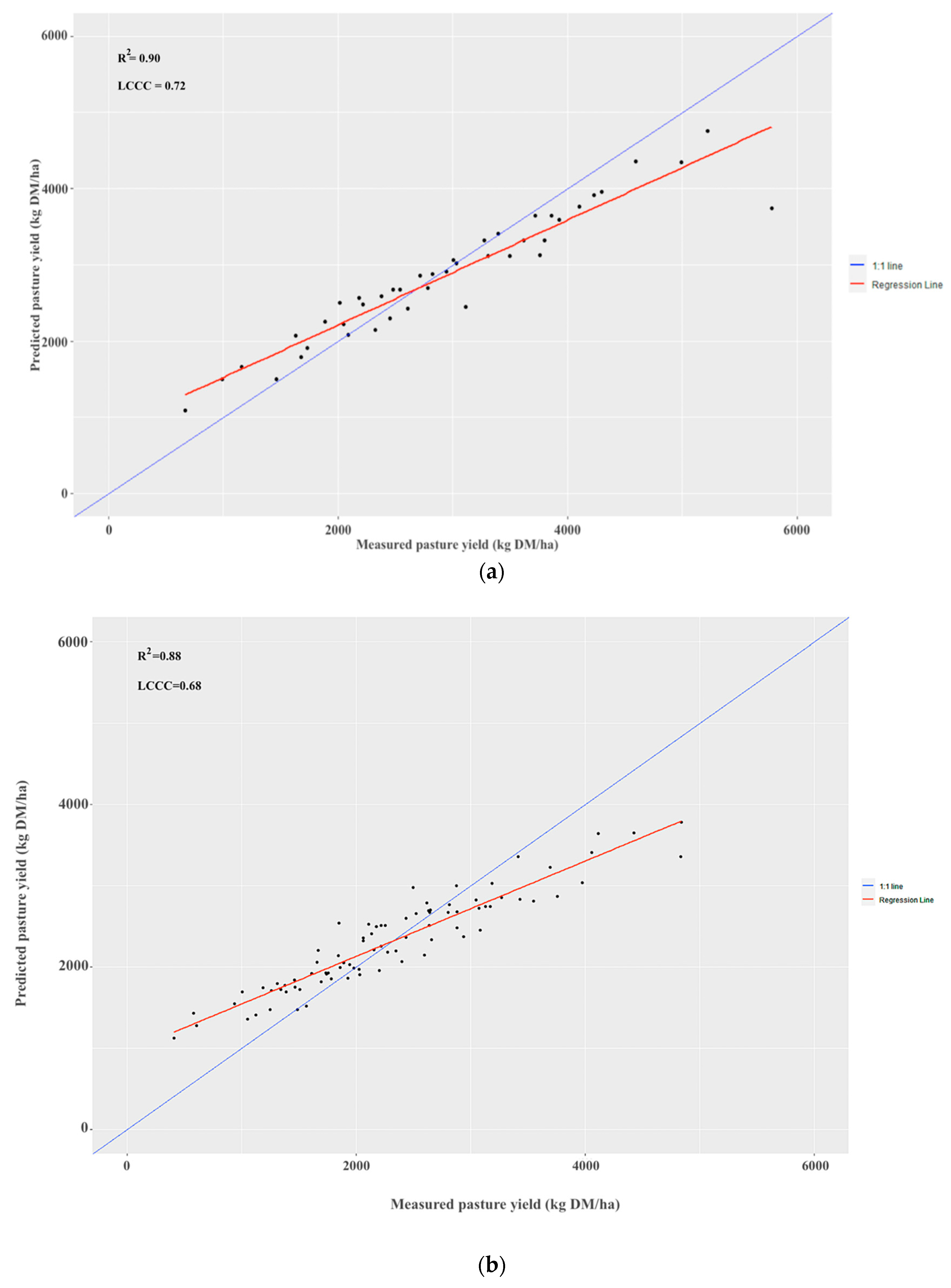
Figure 7a shows the internal model validation where R2 = 0.90 and LCCC = 0.72 were obtained. Moreover, independent validation (n = 84) was conducted to prove the model’s ability to be a global model. Figure 7b shows the correlation between the measured and predicted values, where R2 = 0.88 and LCCC = 0.68 were obtained. The R2 and LCCC values suggested that the model could adequately predict a fully independent validation dataset.
Pasture biomass measured in all seasons and types of management (dryland/irrigated) was considered collectively in both validation datasets. The maximum yield range of the internal validation dataset was close to 6000 kg DM/ha (Figure 7a), which was larger than the independent validation dataset. Although the maximum predicted value was not as close to the regression line, there were limited data at this high range. Furthermore, the prediction range was diminished in the independent validation due to limited relevant data (locations and seasons) (Figure 7b). Nevertheless, the maximum range of biomass prediction exceeded 3000 kg DM/ha in both internal and independent validation (Figure 7), which provides confidence in the robustness of the model. The values of R2 and LCCC for both validations indicate the versatility of the model to be one single global model.
Quantitative comparisons are shown in Table 3. The minimum and maximum measured biomass are shown to highlight the extensive range of biomass values considered in the model. The w and p values from the SW test also show that the data considered for the model calibrations were statistically significant.
Model accuracy indicators, RMSE and NRMSE, provide additional information on the robustness of the model. An RMSE < 500 kg DM/ha was achieved overall (RMSE = 439.49 kg DM/ha and 457.05 kg DM/ha for internal and independent validations, respectively). The entire independent validation data were entered directly into the already calibrated model to assess accuracy, as shown in Table 3.

3.3. Validations Based on Season and Management

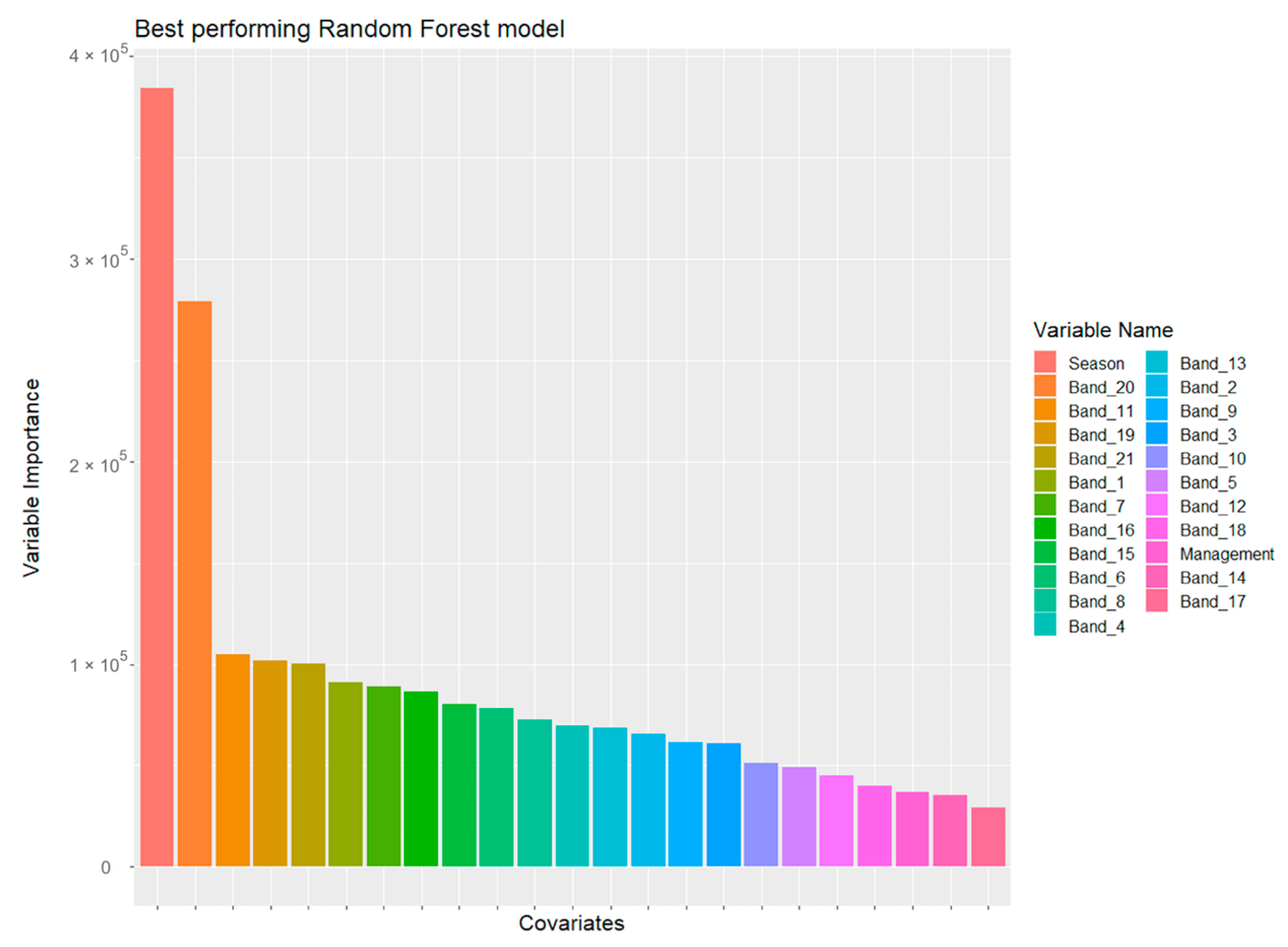
The VI plot (Figure 8) indicated that season was the most important variable. However, it should be mentioned that while the ranks of variables differed, all the variables in Figure 8 were important in the biomass prediction model and should not be eliminated. The type of farm management (irrigated or dryland) was another important variable that passed the Boruta feature selection and was important for the biomass prediction model. Therefore, separate plots were generated for all seasons and farm management (dryland or irrigated) to assess the model accuracy separately.
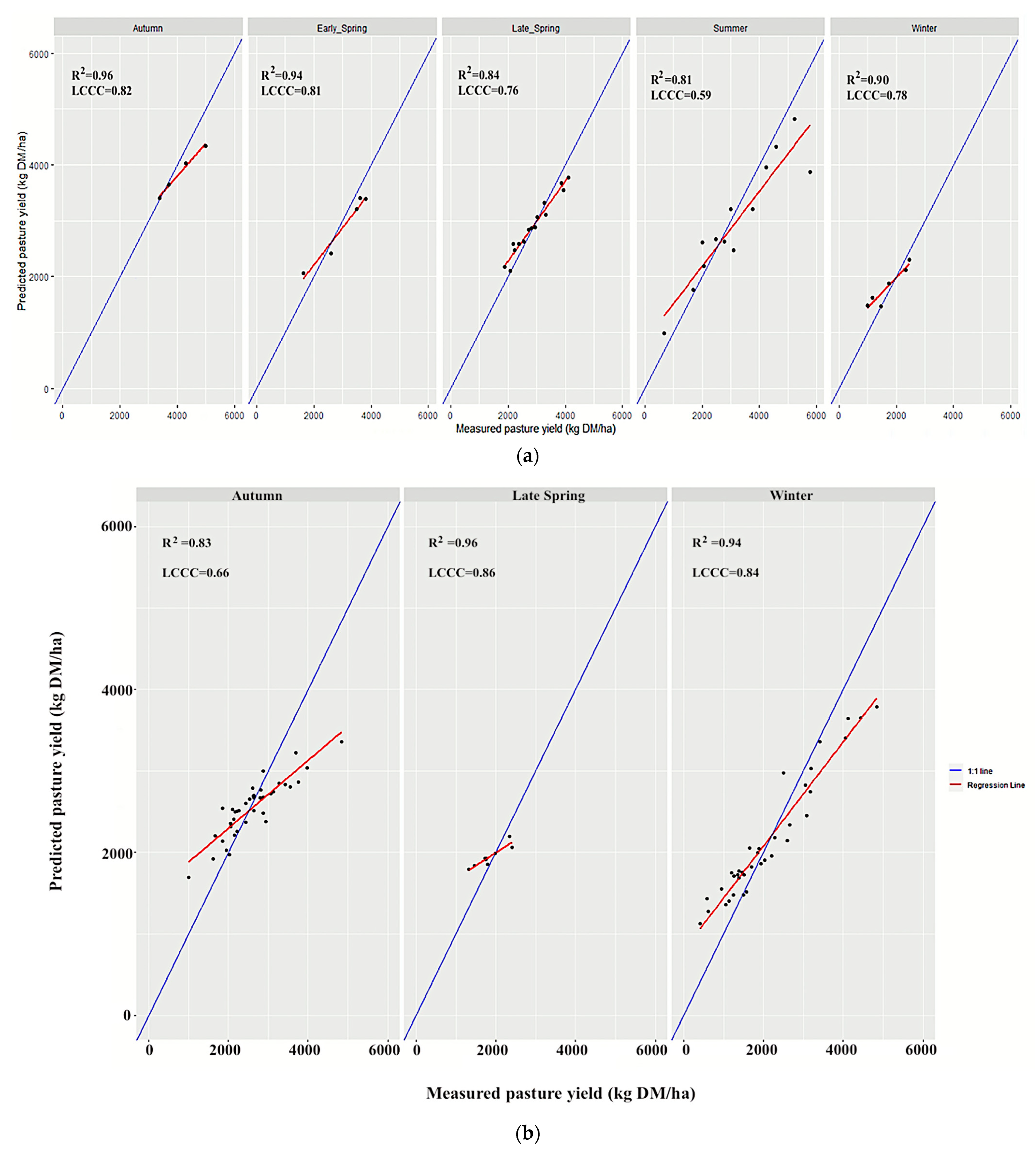
Figure 9 demonstrates the validations based on different seasons combining both types of farm management. The quantitative agreement between the measured and predicted pasture biomass at 0.81 ≤ R2 ≤ 0.96 and 0.59 ≤ LCCC ≤ 0.82 for internal validation (Figure 9a) as well as 0.83 ≤ R2 ≤ 0.96 and 0.66 ≤ LCCC ≤ 0.86 for independent validation (Figure 9b) are evidence of the efficacy of the present ML model in predicting pasture biomass across different seasons. The agreement was improved in seasons that contained more data. The limited data are a result of clouds obstructing satellite images and restricted farm access during the COVID-19 pandemic in early 2020. Due to the lack of relevant data, it was impossible to present independent validation throughout all seasons.
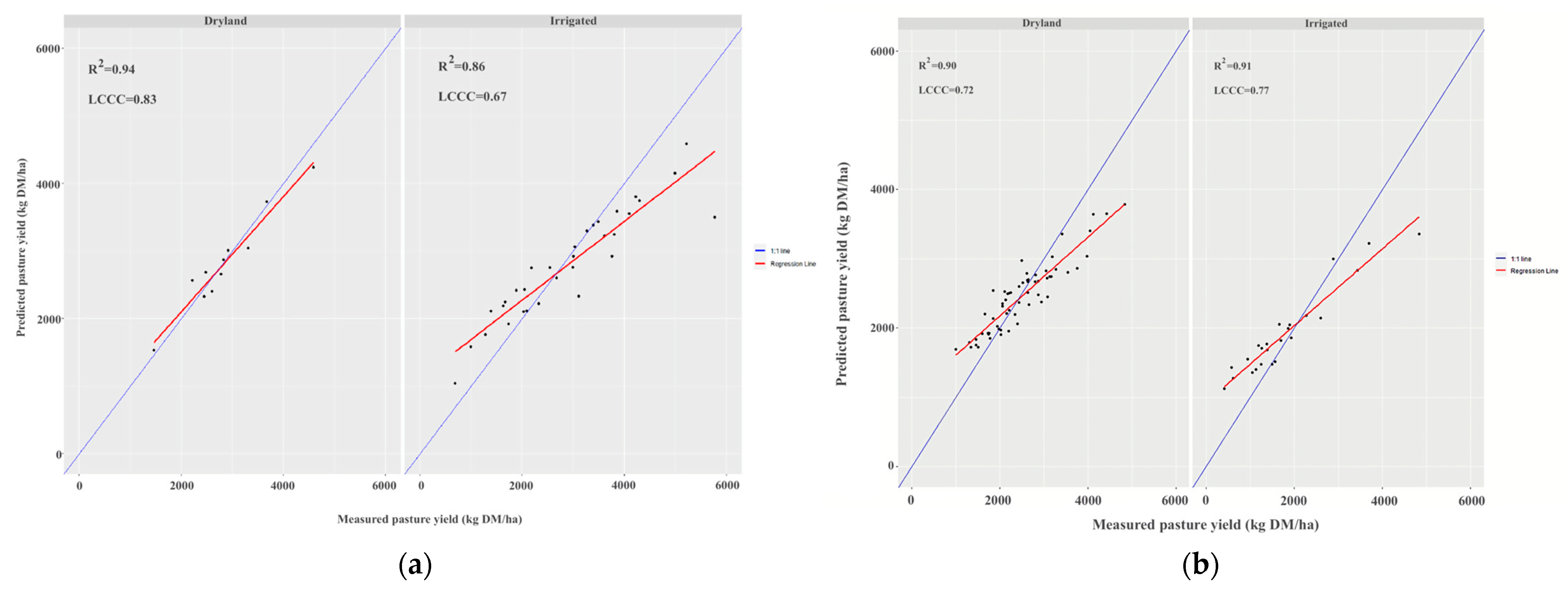
Figure 10 contains the agreement for internal (Figure 10a) and independent (Figure 10b) validations in each farm management type across all farms in all seasons. While internal validation (Figure 10a) contained more information from the irrigation farm management, the scenario was the opposite for the independent validation, as presented in Figure 10b. Regarding internal validation, R2 = 0.94 and LCCC = 0.83 for dryland, and R2 = 0.86 and LCCC = 0.67 for irrigated farm management were obtained. On the other hand, the independent validation exhibited R2 of 0.90 and 0.91 and LCCC values of 0.83 and 0.67 for dryland and irrigated management. The excellent agreement in both validation scenarios indicated that the present model was insensitive and unbiased to the type of farm management.

3.4. SWIR Band Validation

Several tests across different farms were performed to determine the importance of SWIR bands in pasture biomass estimation. SWIR bands were partially or completely removed from the variable set through many model iterations. Index Number Band_20 (B11 SWIR), Band_21 (B12 SWIR), and Band_3 (B12 SWIR/B8A NIR) were left out of the test to determine the importance of SWIR bands. The internal validation results are presented in Figure 11. The removal of SWIR bands reduced the accuracy of the model significantly. The accuracy indicators show that R2 = 0.79 and LCCC = 0.57 were obtained, which are approximately 12% and 21% reductions from the original prediction model. In addition, RMSE = 635.46 kg DM/ha was achieved through this test, which was approximately 45% augmentation on the original pasture biomass prediction model presented in Section 3.2 and Table 4.
A comparison table has also been presented in Table 4 to demonstrate the importance of SWIR bands by comparing two models, one with SWIR bands and one without. The model with SWIR bands predicted maximum pasture biomass up to 4348.25 kg DM/ha from a specific day in the summer season of the PS04 farm. The alternative model, excluding SWIR bands (Band_20, Band_21) and Band_3, was used to predict the pasture biomass of the same day and location, and the maximum biomass obtained was 3379.62 kg DM/ha, which was approximately 22% less than the original prediction model.

3.5. Model Automation

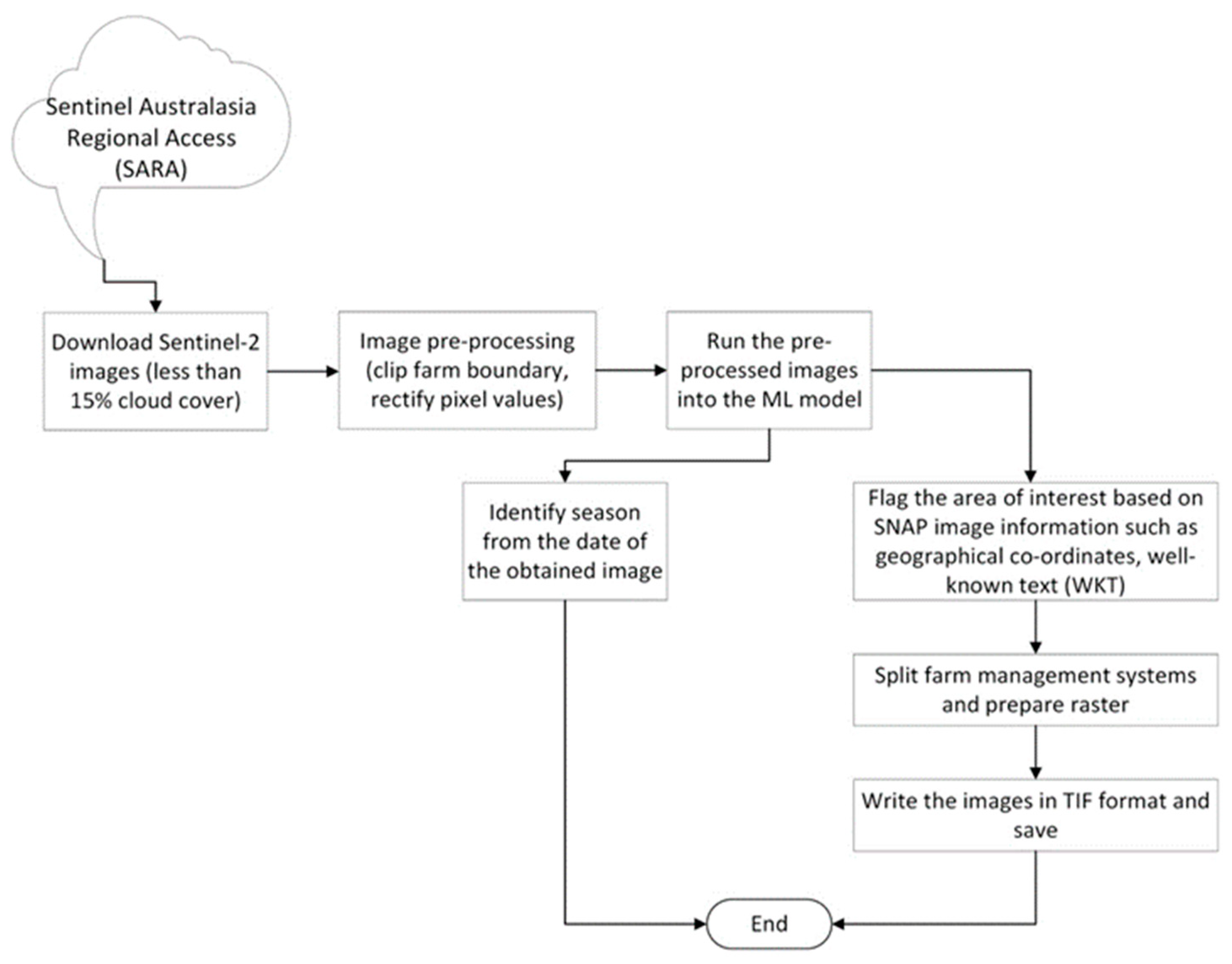
The model introduced in this study was used in an automated data processing flow. Farms involved in the study were mapped, and each paddock management was noted. It was common for dryland farms to have a small proportion of irrigated paddocks and vice versa. The SARA database (https://copernicus.nci.org.au/sara.client/#/home, accessed on 6 October 2020) was reviewed daily using the farm boundary, and when an image with less than 15% cloud was identified, the image was downloaded. This review and download process was automated using Python and APIs established by Geoscience Australia. Once downloaded to an internal computer, the images were pre-processed using the ESA SNAP© graph processing tool. Some of the major S2 image processing operations involved resampling, clipping, S2 band arithmetic computation, band merging, and finally, writing in TIF format.
The image was clipped to the farm extent, all bands were resampled to 10 m, the nine important SIs were calculated, and a stack of 12 bands and 9 SI was created. The model was augmented with functions that read the season from the image file name and the management of each paddock from the farm mapping geodatabase. Finally, biomass predictions were made per pixel to accommodate the different management types in each paddock. Prediction per pixel was achieved using the “splancs” library in the R programming language, which performed the spatial point-pattern analysis [116]. Furthermore, the “inpip” function inside the model selected points inside a polygon based on an area of interest and geospatial information. The output prediction map integrated dryland and irrigated biomass predictions in one farm prediction. A flowchart is presented in Figure 12, outlining the steps.
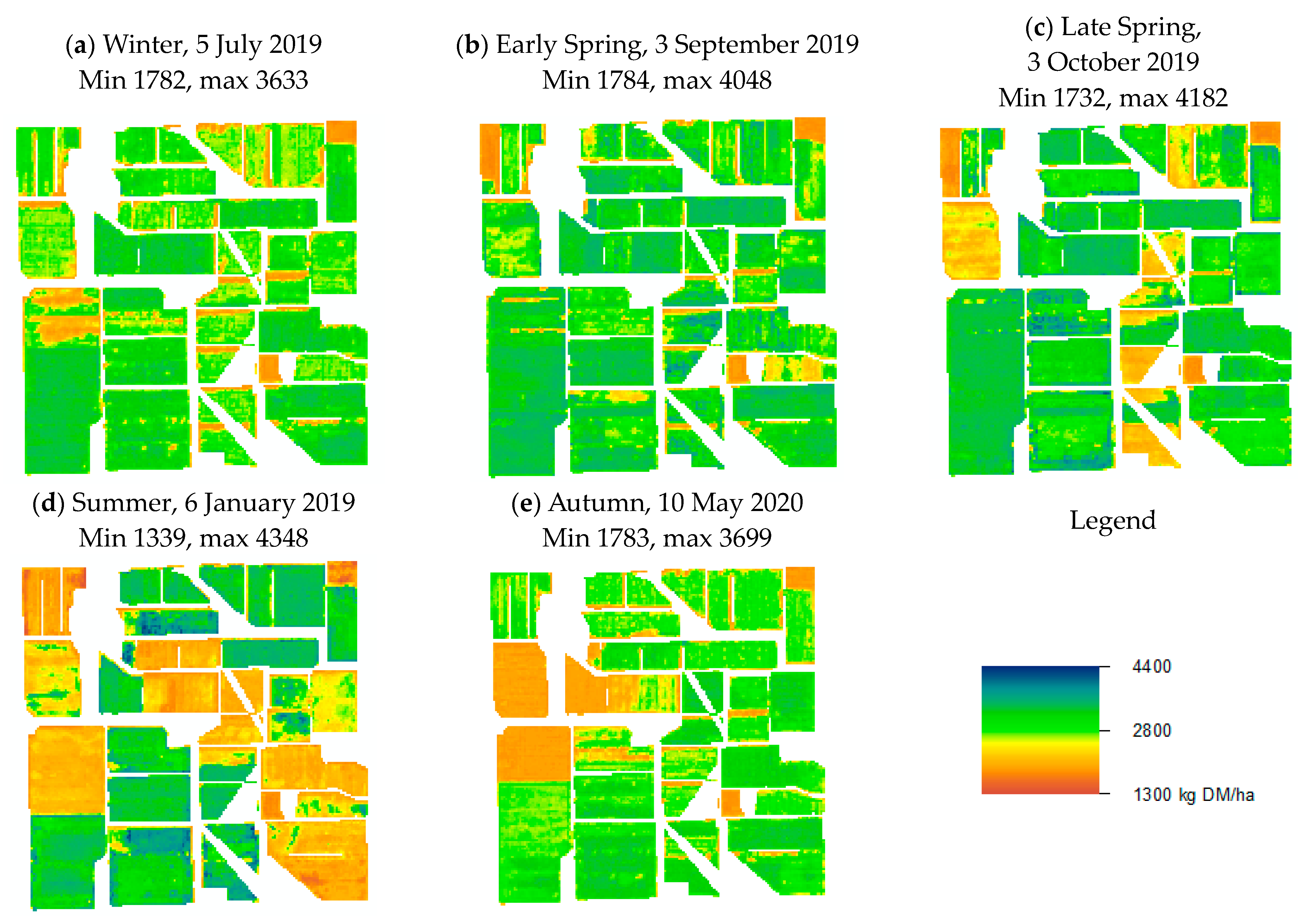
The automation process did not require user-defined commands after a farm was mapped and included in a farm geodatabase (ESRI). An example of the results across five different seasons for the PS04 farm is shown in Figure 13. It could be observed that the maximum biomass prediction exceeded 4000 kg DM/ha for early spring (Figure 13b), late spring (Figure 13c), and summer (Figure 13d). However, the maximum range was found to be 3633.83 kg DM/ha in the winter season (Figure 13a) and 3698.55 kg DM/ha in autumn (Figure 13e). This example was from an irrigated farm. Clear differences in biomass prediction can be seen throughout the image. Many are associated with farm infrastructure, such as water troughs, channel banks, and fences delineating paddock boundaries. Importantly, within-paddock variation is also visible due to uneven pasture growth. In this farm, uneven pasture growth is due to water availability rather than differences in soil type. This farm is flood-irrigated, and therefore, most paddocks have been levelled to allow for optimal water flow. On occasion, water does not reach the end or edges of the paddock due to low water levels in the channel, causing insufficient flow down the paddock. Due to the price and availability of water, not all paddocks were irrigated during this time, highlighting the importance of accommodating changes in management and the full range of biomass amount.

4. Discussion

This study has presented results that are new to the research area. The study has combined a complete dataset collected from active commercial dairy farms with a modelling approach that emphasises the crucial role of remote sensing in solving one of the significant challenges faced by the pasture-based dairy industry, i.e., automated biomass prediction with high accuracy for dense, moist, fast-growing canopies of pasture forages. Excellent prediction qualities have been achieved for all regions, seasons, and management types, producing a single global model for automated pasture biomass prediction. Whilst other studies have investigated minor components common to this study, none have demonstrated real-world outcomes or on a scale that can definitively identify the critical spectral bands required for an accurate prediction. The following sections discuss these novel outcomes in detail.

4.1. Overview of the Prediction Model Accuracy

This study has successfully achieved the stated aim of predicting perennial ryegrass biomass with an accuracy of +/−500 kg DM/ha using internal (RMSE 439.49 kg DM/ha) and independent validation (RMSE 457.05 kg DM/ha). In addition, separate prediction accuracies were presented for seasonal and farm management differences to validate the model’s accuracy. Internal validation across all seasons suggests that the model obtained R2 ≥ 0.81 and LCCC ≥ 0.59. Independent validation was conducted across three seasons, with the model showing an accuracy of R2 ≥ 0.83 and LCCC ≥ 0.66. Similar validations for dryland and irrigated farm management systems provided further evidence of the robustness of the present model where R2 ≥ 0.86 and LCCC ≥ 0.67 (internal validation) and R2 ≥ 0.90 and LCCC ≥ 0.72 (independent validation) were obtained. It should be noted that the validation data was predominantly acquired from entirely different farms and at least a year after the calibration data collection. Additionally, all data were sourced from commercial farms in paddocks under grazing, based on the specific farmer practices. Therefore, there was almost always a day offset between data collection and image acquisition. Nevertheless, R2 and LCCC showed excellent agreements between the predicted and measured pasture biomass for internal and independent validation despite the variability of the conditions and environments under which data were collected.

4.2. Significance of S2 SWIR Bands in Improving Prediction Accuracy

The SWIR validation results were included in Figure 11 and Table 4 to demonstrate the significance of SWIR bands. They support the hypothesis that using SWIR bands would improve the ability to predict pasture yields above 3000 kg DM/ha and, therefore, enable measurements of high-yielding pastures at any stage in the growth cycle in irrigated and dryland production. Dairy pastures before harvest are dense, high moisture swards that can often exceed LAI > 3 and quickly reach the saturation point for common vegetation indices [41]. Saturation is evident at levels >0.7 NDVI [117] and biomass saturation at 2500 kg DM ha [11]. While Edirisinghe et al. [30] and Sinde-Gonzales et al. [12] reported calibration data that exceeded 3000 kg DM/ha, prediction ranges rarely exceeded these levels using NDVI-like indices. SWIR bands are known to be influenced by plant water concentration and therefore are likely to extend the saturation sensitivity point [118,119]. The importance of SWIR bands in improving biomass prediction was also supported by Dang et al. [120], Numata et al. [36], and Pandit et al. [121]. Furthermore, SWIR bands were reported to have strong correlations with pasture biomass, regardless of the type and density of the data and environmental factors [122,123,124]. This study found that adding SWIR bands increased the predictable range of biomass above 4000 kg/DM ha.
Of the 23 bands identified in the VI plot process, S2 B11 SWIR and S2 B12 SWIR were ranked second and fifth, respectively, further supporting the hypothesis that the utilisation of SWIR bands would be significant for model prediction. These bands have centre wavelengths of approximately 1600 and 2200 nm, respectively. The 1600 nm range relates to biochemical components, starch, and sugar, and the 2200 nm range to structural components, lignin, and cellulose [125,126]. Among other bands, in the top 10 most important variables, S2 B2 Blue and S2 B9 Water Vapour were present. S2 B2 has a centre wavelength of 490 nm, an area of strong chlorophyll b absorption [127]. S2 B9 has a centre wavelength of 940 nm and measures water vapour’s absorption over land [128]. Both are important areas of sensitivity in dense, moist canopies. Importantly, this study found that the five most important variables did not include the commonly used red or near-infrared bands found in many biomass studies. Variables ranked six to ten had these common bands but as part of an SI rather than the original band; moreover, the S2 B8 NIR is the lowest-ranked variable in the VI plot. The band ranking suggested that bands associated with canopy and plant moisture were the most important for predicting dense, moist, high-biomass vegetation, such as PRG-based dairy pastures.

4.3. Consideration of ML for Data Analysis and Model Development

This study investigated an extensive range of spectral indices and satellite bands using the ML RF model technique to predict pasture biomass. The ML RF model accommodates high-dimensional data [44]. It was essential to use an approach that could accommodate many variables (68 in the original model) due to the complexity of the farming environment under investigation. Conventional statistical models generally fail to meet accuracy requirements in biomass estimation, particularly at the farm scale, to support on-farm decision-making [129,130]. For example, Ali et al. [129] achieved R2 between 0.57 and 0.86 by using ML to predict the grassland yield estimation through satellite data. In contrast, the conventional statistical model demonstrated the best R2 of 0.31. The advantage of an ML model by Ali et al. [129] was shown further because the lowest NRMSE was reported to be 25.05 using a conventional statistical model and 11.07 using an ML model. However, it should be noted that Ali et al. [129] only considered a single farm with an area of 100 ha, and yet they could only obtain R2 values at most 0.86. Yang et al. [48] also showed a similar comparison and obtained R2 and RMSE of 0.85 and 355 kg DM/ha for the best-performing ML model compared to R2 = 0.58 and RMSE = 536 kg DM/ha through the traditional statistical model. Due to the large number of variables used in the present study, a direct comparison between a conventional statistical approach and an ML approach was not possible. This limitation proves that the ML approach has enhanced the prediction accuracy of the study by effectively accommodating a large data set with 23 input variables.

4.4. Impact of Soils, Climate, and Farm Activities on Satellite Images and Biomass Estimation

This study has benefited from using on-ground data covering various soils, management practices, regions, seasons, and years. The number and type of data points have provided a wide range of biomass not found in other studies. For example, the analysis presented by Chen et al. [25] did not consider large-scale farm areas, and the pasture biomass prediction barely went beyond 4000 kg DM/ha. In addition, the model quality indicators were less accurate than the present study. Chen et al. [25] reported 0.63 ≤ R2 ≤ 0.68 and 0.22 ≤ R2 ≤ 0.40 through their ML internal and independent validations, respectively. Wang et al. [131] obtained R2 = 0.67 in their best-performing ML models; however, the work did not involve any grazing during the growing season. The earlier work by Numata et al. [36] considered grazing intensity, assuming a minimum effect of grazing rotation on the pasture biophysical variables of an actual farm; however, this study does not consider this as a typical scenario for a commercial farm. Xu et al. [47] presented different regression models for different regions. Each region had three equations (linear, power, and exponential) with no possible resolution toward a global or single prediction model within the area of interest. The mathematical interpretation by Grigera et al. [37] to build a correlation between NDVI and fraction absorbed by the canopy (fPAR) was derived from the literature and parametrised based on assumptions. In addition, the determination of radiation use efficiency (RUE) was limited to the local conditions with restricted time steps, and the empirical correlations require further clarification. As such, the correlation presented by Grigera et al. [37] was limited to certain locations, the quality of the data in the literature, and specific time scales. The model will not have the potential to become a global model for predicting pasture biomass. Crabbe et al. [21] primarily relied on field measurements over October and February; therefore, the effect of seasonal cycles was still limited in their prediction model. While comparing different ML techniques was interesting, the precise information on pasture biomass and other model quality indicators, such as RMSE and LCCC, was not reported. Based on the discussions above, the present study fairly outperformed those models by considering one single prediction model across all regions with an entire annual cycle, different types of farm management, and large-scale active farm data that included grazing.
Of the data collected, internal and independent validations demonstrated insensitivity to farm management (dryland and irrigated) and environmental factors (soil type and colour). This result was somewhat surprising, considering that 11 commercial farms in this study had differing soil types and colours. The VI plot assessment (Figure 8) determined that management (dryland and irrigated) was the third least important variable (19th of 21 variables). Separate validation plots were presented in Figure 10, where good accuracy was established in both dryland and irrigated management, indicating the robustness of the prediction model for large-scale working farms, regardless of the kind of management. The soil types in the farms varied from dense and sodic subsoils to strongly acidic brown chromosols, wet soils such as hydrosols, and friable and structured iron-rich soils such as red Ferrosols. Furthermore, variations in soil colour will be exacerbated with varying soil moisture. For example, a dry brown chromosol will be different in colour compared to a wet brown chromosol. Since dryland and irrigated farm management were considered for the model development, substantial variations of soil colour have been accommodated in the final model. Even so, the model was still able to obtain high accuracy, indicating that the prediction model was not biased toward any specific type of soil (soil colour or properties) or geographic location (such as southeast Australia).

4.5. Limitations of the Model

While management was of little importance to the model, the season was the most important variable identified in the VI plot of the best-performing model. Correlations for each of the five seasons used were significant (>0.8). The lowest correlation was found for the summer season (Dec, Jan, and Feb), where the most extensive data range was measured. High biomass occurred in summer irrigated pastures while dryland pastures commonly senesce due to lack of moisture and have low biomass at this time. While Figure 9 showed clear groupings associated with each season demonstrating good model outcomes, further improvement is likely if the climatic characteristics recorded at the overpass were used rather than coarse seasons. The enhancement will have the most significant impact in the summer when the difference in soil moisture concentration and evapotranspiration is most marked between irrigated and dryland management systems.
Even though this study has demonstrated the transferability of the model across regions within southeastern Australia, seasons, and management types due to an extensive dataset, the present model was limited by cloud-free imagery. While seasons like late spring (October, November) and summer (December–February) had numerous cloud-free satellite overpasses, the major challenge was during the winter season (June–July). As a result, the range of biomass estimation was limited during the winter. Furthermore, the satellite images were only considered if the field data collection occurred after S2 overpassing on the same day or within a time (≤5 days) that limited potential pasture growth to less than 200 kg DM/ha.
Additionally, the present study contains field data from commercial farms; therefore, activities such as grazing events will also affect the paddock’s variability. Furthermore, grazing only sometimes follows a sequential schedule, depending on pasture growth, suitable weather, and farm requirements. Consequently, available satellite data might be further impacted. The ideal approach was to coincide the field data collection date with the same day of the satellite overpass. However, this was difficult to achieve due to certain farm activities, weather conditions, and set satellite overpass schedules. Among the whole dataset considered in this study, less than ten field data collections coincided with the satellite overpassing, which might also have affected the model prediction accuracy.
For pasture to be the cheapest feeding source for dairy animals, grazing must be well-managed to ensure efficient pasture utilisation. Therefore, the limited temporal availability of biomass estimations may significantly impact the practical application of the model outcomes developed. The addition of Synthetic-aperture radar (SAR), such as Sentinel-1 (S1), which can pass through the cloud and provide regular observation, is under development to overcome this significant issue. However, SAR satellites frequently face challenges due to speckle, which is caused by the interference between the randomly distributed scatters within each pixel [132]. Hence, building a multivariate hybrid model requires more investigation into image pre-processing, calibration, and integration with the S2 imagery. A similar ML RF modelling approach integrating S1 data will be investigated based on the model’s success described here.

5. Conclusions

This study has presented an ML RF model incorporating S2 images to predict PRG biomass in pastures across southeast Australia on 11 commercial dairy farms. This study has successfully achieved the stated aim of predicting perennial ryegrass biomass with an accuracy of +/−500 kg DM/ha using internal and independent validation. R2 and LCCC showed excellent agreements between the predicted and measured pasture biomass for internal and independent validation despite the variability of the conditions and environments under which data were collected.
This study has also found that the availability of SWIR bands increased the predictable range of biomass above 4000 kg/DM ha. The R2 value and LCCC showed excellent agreement between the predicted and measured pasture biomass amount (kg DM/ha) for internal and independent validations despite the complexity of the data. The results support the hypothesis and exceed the expectation that using SWIR bands would improve the ability to predict pasture yields above 3000 kg DM/ha and, therefore, enable measurements of high-yielding pastures at any stage in the growth cycle in irrigated and dryland production. The VI plot band ranking suggested that bands associated with canopy and plant moisture were the most important for predicting dense, moist, high-biomass vegetation such as PRG-based dairy pastures.
The ML RF approach improved the prediction accuracy of the study by effectively accommodating a large set of variables (12 bands, 9 SI, season, and management). This study outperformed previously reported models by considering one single prediction model across all regions with a complete annual cycle, different types of farm management, and typical commercial farm activities, including grazing. Additionally, the model was still able to obtain high model quality, indicating that the prediction model was not biased toward any specific type of soil (soil colour or properties) or geographic location.
Further improvement is possible if the climatic characteristics recorded during the overpass were used rather than coarse seasons. The enhancement will have the most significant impact in the summer when the difference in soil moisture concentration and evapotranspiration is the greatest between irrigated and dryland management systems. Among the whole dataset considered in this study, less than ten field data collections coincided with the satellite overpassing, which might also have affected the model prediction accuracy. Based on the model’s success described here, a similar ML RF modelling approach will be investigated to integrate S1 data.

Author Contributions

E.M.M.-M.: conceptualisation, data curation, formal analysis, software, methodology, writing—original draft, supervision, funding acquisition, project administration; M.F.H.: conceptualisation, software, methodology, validation, formal analysis, writing—original draft; S.K.: conceptualisation, software, writing—draft review and editing. All authors have read and agreed to the published version of the manuscript.

Funding

The work was funded by the Dairy Feedbase Program: A joint venture between Dairy Australia, Gardiner Dairy Foundation, and Agriculture Victoria.

Data Availability Statement

Data may be made available on request at the completion of the research program when all publication is complete.

Acknowledgments

The authors would like to thank the Pasture Smarts project team that has contributed in many ways over the years; Misbah Aiad, Craig Beverley, Stewie Burch, Liz Byrne, Amy Copland, Richard Dabrowski, David Hunter, Joe Jacobs, Chinthaka Jayasinghe, Alister Lawson, Clare Leddin, Stephanie Muir, Graeme Phyland, Elly Polonowita, Kelly Rentsch, Kevin Smith, Dani Stayches, Anna Thomson, Anna Weeks, and Muhammad Islam. The authors would also like to acknowledge Kevin Kelly, who made significant contributions to Victoria’s dairy industry, particularly in pasture and forage crop agronomy, and measurement of soil emissions. Kelly sadly passed away in the first year of the project.

Conflicts of Interest

The authors declare that they have no known competing financial interests or personal relationships that could have appeared to influence the work reported in this paper.

References

  1. Chang-Fung-Martel, J.; Harrison, M.T.; Rawnsley, R.; Smith, A.P.; Meinke, H. The impact of extreme climatic events on pasture-based dairy systems: A review. Crop Pasture Sci. 2017, 68, 1158–1169. [Google Scholar] [CrossRef]
  2. Dairy Feeding Update Briefing Notes 2015. Dairy Australia. Available online: https://www.dairyaustralia.com.au/resource-repository/2020/07/09/dairy-feeding-update-briefing-notes-2015 (accessed on 15 June 2022).
  3. Fulkerson, W.J.; McKean, K.; Nandra, K.S.; Barchia, I.M. Benefits of accurately allocating feed on a daily basis to dairy cows grazing pasture. Aust. J. Experiment. Agri. 2005, 45, 331–336. [Google Scholar] [CrossRef]
  4. Rogers, M.J.; Lawson, A.; Ho, C.; Kelly, K.; Wales, W.; Jacobs, J. The changing role of perennial ryegrass in dairy pastures in northern Victoria, Australia. Grass Forag. Sci. 2022, 77, 131–140. [Google Scholar] [CrossRef]
  5. Beukes, P.C.; McCarthy, S.; Wims, C.M.; Gregorini, P.; Romera, A.J. Regular estimates of herbage mass can improve profitability of pasture-based dairy systems. Anim. Prod. Sci. 2019, 59, 359–367. [Google Scholar] [CrossRef]
  6. De Rosa, D.; Basso, B.; Fasiolo, M.; Friedl, J.; Fulkerson, B.; Grace, P.R.; Rowlings, D.W. Predicting pasture biomass using a statistical model and machine learning algorithm implemented with remotely sensed imagery. Comput. Electron. Agric. 2021, 180, 105880. [Google Scholar] [CrossRef]
  7. Earle, D.F.; McGowan, A.A. Evaluation and calibration of an automated rising plate meter for estimating dry-matter yield of pasture. Aust. J. Exp. Agric. 1979, 19, 337–343. [Google Scholar] [CrossRef]
  8. Ehlert, D.; Hammen, V.; Adamek, R. Online sensor pendulum-meter for determination of plant mass. Precis. Agric. 2003, 4, 139–148. [Google Scholar] [CrossRef]
  9. Serrano, J.M.; Shahidian, S.; Marques da Silva, J.R. Monitoring pasture variability: Optical OptRx® crop sensor versus Grassmaster II capacitance probe. Environ. Mon. Assess. 2016, 188, 117. [Google Scholar] [CrossRef]
  10. Legg, M.; Bradley, S. Ultrasonic arrays for remote sensing of pasture biomass. Remote Sens. 2019, 12, 111. [Google Scholar] [CrossRef] [Green Version]
  11. Alckmin, G.T.; Lucieer, A.; Rawnsley, R.; Kooistra, L. Perennial ryegrass biomass retrieval through multispectral UAV data. Comput. Electron. Agric. 2022, 193, 106574. [Google Scholar] [CrossRef]
  12. Sinde-González, I.; Gil-Docampo, M.; Arza-García, M.; Grefa-Sánchez, J.; Yánez-Simba, D.; Pérez-Guerrero, P.; Abril-Porras, V. Biomass estimation of pasture plots with multitemporal UAV-based photogrammetric surveys. Int. J. Appl. Earth Obs. Geoinfo. 2021, 101, 102355. [Google Scholar] [CrossRef]
  13. Rouse, J.W., Jr.; Haas, R.H.; Schell, J.A.; Deering, D.W. Monitoring the Vernal Advancement and Retrogradation (Green Wave Effect) of Natural Vegetation, Type II Report for the Period April 1973–September 1973; Texas A&M University, Remote Sensing Center: College Station, Texas, USA, 1973. [Google Scholar]
  14. Chen, J.M.; Cihlar, J. Retrieving leaf area index of boreal conifer forests using Landsat TM images. Remote Sens. Environ. 1996, 55, 153–162. [Google Scholar] [CrossRef]
  15. Gara, T.W.; Darvishzadeh, R.; Skidmore, A.K.; Wang, T.; Heurich, M. Accurate modelling of canopy traits from seasonal Sentinel-2 imagery based on the vertical distribution of leaf traits. ISPRS J. Photogramm. Remote Sens. 2019, 157, 108–123. [Google Scholar] [CrossRef]
  16. Liu, Y.; Gong, W.; Xing, Y.; Hu, X.; Gong, J. Estimation of the forest stand mean height and aboveground biomass in Northeast China using SAR Sentinel-1B, multispectral Sentinel-2A, and DEM imagery. ISPRS J. Photogramm. Remote Sens. 2019, 151, 277–289. [Google Scholar] [CrossRef]
  17. Chen, D.; Huang, J.; Jackson, T.J. Vegetation water content estimation for corn and soybeans using spectral indices derived from MODIS near-and short-wave infrared bands. Remote Sens. Environ. 2005, 98, 225–236. [Google Scholar] [CrossRef]
  18. Delegido, J.; Verrelst, J.; Meza, C.M.; Rivera, J.P.; Alonso, L.; Moreno, J. A red-edge spectral index for remote sensing estimation of green LAI over agroecosystems. Euro. J. Agron. 2013, 46, 42–52. [Google Scholar] [CrossRef]
  19. Hunt, M.L.; Blackburn, G.A.; Carrasco, L.; Redhead, J.W.; Rowland, C.S. High resolution wheat yield mapping using Sentinel-2. Remote Sens. Environ. 2019, 233, 111410. [Google Scholar] [CrossRef]
  20. Hill, M.J.; Vickery, P.J.; Furnival, E.P.; Donald, G.E. Pasture Land Cover in Eastern Australia from NOAA-AVHRR NDVI and Classified Landsat TM. Remote Sens. Environ. 1999, 67, 32–50. [Google Scholar] [CrossRef]
  21. Crabbe, R.A.; Lamb, D.; Edwards, C. Discrimination of species composition types of a grazed pasture landscape using Sentinel-1 and Sentinel-2 data. Int. J. Appl. Earth Obs. Geoinf. 2020, 84, 101978. [Google Scholar] [CrossRef]
  22. Yeganeh, H.; Khajedein, S.; Jamale Amiri, F.; Shariff, A.R.B.M. Monitoring rangeland ground cover vegetation using multitemporal MODIS data. Arab. J. Geosci. 2014, 7, 287–298. [Google Scholar] [CrossRef]
  23. Cicore, P.; Serrano, J.; Shahidian, S.; Sousa, A.; Costa, J.L.; da Silva, J.R.M. Assessment of the spatial variability in tall wheatgrass forage using LANDSAT 8 satellite imagery to delineate potential management zones. Environ. Monit. Assess. 2016, 188, 513. [Google Scholar] [CrossRef] [PubMed]
  24. Ali, I.; Barrett, B.; Cawkwell, F.; Green, S.; Dwyer, E.; Neumann, M. Application of repeat-pass TerraSAR-X staring spotlight interferometric coherence to monitor pasture biophysical parameters: Limitations and sensitivity analysis. IEEE J. Sel. Top. Appl. Earth Obs. Remote Sens. 2017, 10, 3225–3231. [Google Scholar] [CrossRef] [Green Version]
  25. Chen, Y.; Guerschman, J.; Shendryk, Y.; Henry, D.; Harrison, M.T. Estimating pasture biomass using Sentinel-2 imagery and machine learning. Remote Sens. 2021, 13, 603. [Google Scholar] [CrossRef]
  26. Porter, T.F.; Chen, C.; Long, J.A.; Lawrence, R.L.; Sowell, B.F. Estimating biomass on CRP pastureland: A comparison of remote sensing techniques. Biomass Bioenerg. 2014, 66, 268–274. [Google Scholar] [CrossRef]
  27. Reinermann, S.; Asam, S.; Kuenzer, C. Remote sensing of grassland production and management—A review. Remote Sens. 2020, 12, 1949. [Google Scholar] [CrossRef]
  28. Vickery, P.J.; Hedges, D.A.; Duggin, M.J. Assessment of the fertiliser requirement of improved pasture from remote sensing information. Remote Sens. Environ. 1980, 9, 131–148. [Google Scholar] [CrossRef]
  29. Taylor, B.F.; Dini, P.W.; Kidson, J.W. Determination of seasonal and interannual variation in New Zealand pasture growth from NOAA-7 data. Remote Sens. Environ. 1985, 18, 177–192. [Google Scholar] [CrossRef]
  30. Edirisinghe, A.; Clark, D.; Waugh, D. Spatio-temporal modelling of biomass of intensively grazed perennial dairy pastures using multispectral remote sensing. Int. J. Appl. Earth Obs. Geoinf. 2012, 16, 5–16. [Google Scholar] [CrossRef]
  31. Edirisinghe, A.; Hill, M.J.; Donald, G.E.; Hyder, M. Quantitative mapping of pasture biomass using satellite imagery. Int. J. Remote Sens. 2011, 32, 2699–2724. [Google Scholar] [CrossRef]
  32. Guerini Filho, M.; Kuplich, T.M.; Quadros, F.L.D. Estimating natural grassland biomass by vegetation indices using Sentinel 2 remote sensing data. Int. J. Remote Sens. 2020, 41, 2861–2876. [Google Scholar] [CrossRef]
  33. Chen, L.; Wang, Y.; Ren, C.; Zhang, B.; Wang, Z. Optimal combination of predictors and algorithms for forest above-ground biomass mapping from Sentinel and SRTM data. Remote Sens. 2019, 11, 414. [Google Scholar] [CrossRef] [Green Version]
  34. Sibanda, M.; Mutanga, O.; Rouget, M. Examining the potential of Sentinel-2 MSI spectral resolution in quantifying above ground biomass across different fertilizer treatments. ISPRS J. Photogramm. Remote Sens. 2015, 110, 55–65. [Google Scholar] [CrossRef]
  35. Maynard, C.L.; Lawrence, R.L.; Nielsen, G.A.; Decker, G. Modeling vegetation amount using bandwise regression and ecological site descriptions as an alternative to vegetation indices. GISci. Remote Sens. 2007, 44, 68–81. [Google Scholar] [CrossRef]
  36. Numata, I.; Roberts, D.A.; Chadwick, O.A.; Schimel, J.; Sampaio, F.R.; Leonidas, F.C.; Soares, J.V. Characterization of pasture biophysical properties and the impact of grazing intensity using remotely sensed data. Remote Sens. Environ. 2007, 109, 314–327. [Google Scholar] [CrossRef]
  37. Grigera, G.; Oesterheld, M.; Pacín, F. Monitoring forage production for farmers’ decision making. Agric. Syst. 2007, 94, 637–648. [Google Scholar] [CrossRef]
  38. Punalekar, S.M.; Verhoef, A.; Quaife, T.L.; Humphries, D.; Bermingham, L.; Reynolds, C.K. Application of Sentinel-2A data for pasture biomass monitoring using a physically based radiative transfer model. Remote Sens. Environ. 2018, 218, 207–220. [Google Scholar] [CrossRef]
  39. Boschetti, M.; Bocchi, S.; Brivio, P.A. Assessment of pasture production in the Italian Alps using spectrometric and remote sensing information. Agric. Ecosyst. Environ. 2007, 118, 267–272. [Google Scholar] [CrossRef]
  40. Tucker, C.J. Red and photographic infrared linear combinations for monitoring vegetation. Remote Sens. Environ. 1979, 8, 127–150. [Google Scholar] [CrossRef] [Green Version]
  41. Sellers, P.J. Canopy reflectance, photosynthesis and transpiration. Int. J. Remote Sens. 1985, 6, 1335–1372. [Google Scholar] [CrossRef] [Green Version]
  42. Broge, N.H.; Leblanc, E. Comparing prediction power and stability of broadband and hyperspectral vegetation indices for estimation of green leaf area index and canopy chlorophyll density. Remote Sens. Environ. 2001, 76, 156–172. [Google Scholar] [CrossRef]
  43. Gargiulo, J.; Clark, C.; Lyons, N.; de Veyrac, G.; Beale, P.; Garcia, S. Spatial and temporal pasture biomass estimation integrating electronic plate meter, planet cubesats and sentinel-2 satellite data. Remote Sens. 2020, 12, 3222. [Google Scholar] [CrossRef]
  44. Belgiu, M.; Drăguţ, L. Random forest in remote sensing: A review of applications and future directions. ISPRS J. Photogramm. Remote Sens. 2016, 114, 24–31. [Google Scholar] [CrossRef]
  45. Maxwell, A.E.; Warner, T.A.; Fang, F. Implementation of machine-learning classification in remote sensing: An applied review. Int. J. Remote Sens. 2018, 39, 2784–2817. [Google Scholar] [CrossRef] [Green Version]
  46. Deb, D.; Deb, S.; Chakraborty, D.; Singh, J.P.; Singh, A.K.; Dutta, P.; Choudhury, A. Aboveground biomass estimation of an agro-pastoral ecology in semi-arid Bundelkhand region of India from Landsat data: A comparison of support vector machine and traditional regression models. Geocarto Int. 2022, 37, 1043–1058. [Google Scholar] [CrossRef]
  47. Xu, K.; Su, Y.; Liu, J.; Hu, T.; Jin, S.; Ma, Q.; Zhai, Q.; Wang, R.; Zhang, J.; Li, Y.; et al. Estimation of degraded grassland aboveground biomass using machine learning methods from terrestrial laser scanning data. Ecol. Indicat. 2020, 108, 105747. [Google Scholar] [CrossRef]
  48. Yang, S.; Feng, Q.; Liang, T.; Liu, B.; Zhang, W.; Xie, H. Modeling grassland above-ground biomass based on artificial neural network and remote sensing in the Three-River Headwaters Region. Remote Sens. Environ. 2018, 204, 448–455. [Google Scholar] [CrossRef]
  49. Aguirre-Salado, C.A.; Treviño-Garza, E.J.; Aguirre-Calderón, O.A.; Jiménez-Pérez, J.; González-Tagle, M.A.; Valdéz-Lazalde, J.R.; Sánchez-Díaz, G.; Haapanen, R.; Aguirre-Salado, A.I.; Miranda-Aragón, L. Mapping aboveground biomass by integrating geospatial and forest inventory data through a k-nearest neighbor strategy in North Central Mexico. J. Arid Land 2014, 6, 80–96. [Google Scholar] [CrossRef]
  50. Habyarimana, E.; Piccard, I.; Catellani, M.; De Franceschi, P.; Dall’Agata, M. Towards predictive modeling of sorghum biomass yields using fraction of absorbed photosynthetically active radiation derived from sentinel-2 satellite imagery and supervised machine learning techniques. Agronomy 2019, 9, 203. [Google Scholar] [CrossRef] [Green Version]
  51. Bretas, I.L.; Valente, D.S.; Silva, F.F.; Chizzotti, M.L.; Paulino, M.F.; D’Áurea, A.P.; Paciullo, D.S.; Pedreira, B.C.; Chizzotti, F.H. Prediction of aboveground biomass and dry-matter content in Brachiaria pastures by combining meteorological data and satellite imagery. Grass Forage Sci. 2021, 76, 340–352. [Google Scholar] [CrossRef]
  52. Victorian Resources Online, 2022. Available online: https://vro.agriculture.vic.gov.au/dpi/vro/vrosite.nsf/pages/soil-home (accessed on 1 October 2022).
  53. Searle, R. Australian Soil Classification Map, Version 1.0.0; Terrestrial Ecosystem Research Network. (Dataset); TERN: Indooroopilly, QLD, Australia, 2021. [CrossRef]
  54. Esri, 2022a. Esri, Collector for ArcGIS Overview. Available online: https://www.esri.com/en-us/arcgis/products/collector-for-arcgis/overview (accessed on 19 May 2022).
  55. Karunaratne, S.; Thomson, A.; Morse-McNabb, E.; Wijesingha, J.; Stayches, D.; Copland, A.; Jacobs, J. The fusion of spectral and structural datasets derived from an airborne multispectral sensor for estimation of pasture dry matter yield at paddock scale with time. Remote Sens. 2020, 12, 2017. [Google Scholar] [CrossRef]
  56. Lawson, A.R.; Giri, K.; Thomson, A.L.; Karunaratne, S.B.; Smith, K.F.; Jacobs, J.L.; Morse-McNabb, E.M. Multi-site calibration and validation of a wide-angle ultrasonic sensor and precise GPS to estimate pasture mass at the paddock scale. Comput. Electron. Agric. 2022, 195, 106786. [Google Scholar] [CrossRef]
  57. Thomson, A.L.; Karunaratne, S.B.; Copland, A.; Stayches, D.; McNabb, E.M.; Jacobs, J. Use of traditional, modern, and hybrid modelling approaches for in situ prediction of dry matter yield and nutritive characteristics of pasture using hyperspectral datasets. Anim. Feed Sci. Technol. 2020, 269, 114670. [Google Scholar] [CrossRef]
  58. Esri, 2022b. Esri, ArcGIS Online. Available online: https://www.arcgis.com/home/ (accessed on 19 May 2022).
  59. Doyle, P.T.; Stockdale, C.R.; Lawson, A.R.; Cohen, D.C. Pastures for Dairy Production in Victoria; Agriculture Victoria, Department of Natural Resources and Environment: Tatura, VIC, Australia, 2001. [Google Scholar]
  60. L3Harris Technologies, Inc., 2022. ENVI®. Available online: https://www.l3harris.com/all-capabilities/envi (accessed on 20 August 2022).
  61. SENTINEL-2 User Handbook, 2015. European Space Agency. Available online: https://sentinel.esa.int/documents/247904/685211/sentinel-2_user_handbook (accessed on 10 June 2022).
  62. Gitelson, A.A.; Merzlyak, M.N.; Chivkunova, O.B. Optical properties and nondestructive estimation of anthocyanin content in plant leaves. Photochem. Photobiol. 2001, 74, 38–45. [Google Scholar] [CrossRef] [PubMed]
  63. Kaufman, Y.J.; Tanre, D. Atmospherically resistant vegetation index (ARVI) for EOS-MODIS. IEEE Trans. Geosci. Remote Sens. 1992, 30, 261–270. [Google Scholar] [CrossRef]
  64. Huete, A.; Didan, K.; Miura, T.; Rodriguez, E.P.; Gao, X.; Ferreira, L.G. Overview of the radiometric and biophysical performance of the MODIS vegetation indices. Remote Sens. Environ. 2002, 83, 195–213. [Google Scholar] [CrossRef]
  65. Jiang, Z.; Huete, A.R.; Didan, K.; Miura, T. Development of a two-band enhanced vegetation index without a blue band. Remote Sens. Environ. 2008, 112, 3833–3845. [Google Scholar] [CrossRef]
  66. Pinty, B.; Verstraete, M.M. GEMI: A non-linear index to monitor global vegetation from satellites. Vegetation 1992, 101, 15–20. [Google Scholar] [CrossRef]
  67. Gitelson, A.A.; Kaufman, Y.J.; Merzlyak, M.N. Use of a green channel in remote sensing of global vegetation from EOS-MODIS. Remote Sens. Environ. 1996, 58, 289–298. [Google Scholar] [CrossRef]
  68. Gitelson, A.A.; Gritz, Y.; Merzlyak, M.N. Relationships between leaf chlorophyll content and spectral reflectance and algorithms for non-destructive chlorophyll assessment in higher plant leaves. J. Plant Phys. 2003, 160, 271–282. [Google Scholar] [CrossRef]
  69. Sripada, R.P. Determining In-Season Nitrogen Requirements of Corn Using Aerial Color-Intrared Photography. Ph.D. Dissertation, North Carolina State University, Raleigh, NC, USA, 2005. [Google Scholar]
  70. Louhaichi, M.; Borman, M.M.; Johnson, D.E. Spatially located platform and aerial photography for documentation of grazing impacts on wheat. Geocarto Int. 2001, 16, 65–70. [Google Scholar] [CrossRef]
  71. Gitelson, A.A.; Merzlyak, M.N. Remote sensing of chlorophyll concentration in higher plant leaves. Adv. Space Res. 1998, 22, 689–692. [Google Scholar] [CrossRef]
  72. Boegh, E.; Soegaard, H.; Broge, N.; Hasager, C.B.; Jensen, N.O.; Schelde, K.; Thomsen, A. Airborne multispectral data for quantifying leaf area index, nitrogen concentration, and photosynthetic efficiency in agriculture. Remote Sens. Environ. 2002, 81, 179–193. [Google Scholar] [CrossRef]
  73. Daughtry, C.S.; Walthall, C.L.; Kim, M.S.; De Colstoun, E.B.; McMurtrey, J.E., III. Estimating corn leaf chlorophyll concentration from leaf and canopy reflectance. Remote Sens. Environ. 2000, 74, 229–239. [Google Scholar] [CrossRef]
  74. Haboudane, D.; Miller, J.R.; Pattey, E.; Zarco-Tejada, P.J.; Strachan, I.B. Hyperspectral vegetation indices and novel algorithms for predicting green LAI of crop canopies: Modeling and validation in the context of precision agriculture. Remote Sens. Environ. 2004, 90, 337–352. [Google Scholar] [CrossRef]
  75. Datt, B. A new reflectance index for remote sensing of chlorophyll content in higher plants: Tests using Eucalyptus leaves. J. Plant Phys. 1999, 154, 30–36. [Google Scholar] [CrossRef]
  76. Sims, D.A.; Gamon, J.A. Relationships between leaf pigment content and spectral reflectance across a wide range of species, leaf structures and developmental stages. Remote Sens. Environ. 2002, 81, 337–354. [Google Scholar] [CrossRef]
  77. Chen, J. Evaluation of Vegetation Indices and Modified Simple Ratio for Boreal Applications. Can. J. Remote Sens. 1996, 22, 229–242. [Google Scholar] [CrossRef]
  78. Qi, J.; Chehbouni, A.; Huete, A.R.; Kerr, Y.H.; Sorooshian, S. A modified soil adjusted vegetation index. Remote Sens. Environ. 1994, 48, 119–126. [Google Scholar] [CrossRef]
  79. Goel, N.S.; Qin, W. Influences of canopy architecture on relationships between various vegetation indices and LAI and FPAR: A computer simulation. Remote Sens. Rev. 1994, 10, 309–347. [Google Scholar] [CrossRef]
  80. Rondeaux, G.; Steven, M.; Baret, F. Optimization of soil-adjusted vegetation indices. Remote Sens. Environ. 1996, 55, 95–107. [Google Scholar] [CrossRef]
  81. Merzlyak, M.N.; Gitelson, A.A.; Chivkunova, O.B.; Rakitin, V.Y. Non-destructive optical detection of pigment changes during leaf senescence and fruit ripening. Phys. Plant. 1999, 106, 135–141. [Google Scholar] [CrossRef] [Green Version]
  82. Roujean, J.L.; Breon, F.M. Estimating PAR absorbed by vegetation from bidirectional reflectance measurements. Remote Sens. Environ. 1995, 51, 375–384. [Google Scholar] [CrossRef]
  83. Huete, A.R. A soil-adjusted vegetation index (SAVI). Remote Sens. Environ. 1988, 25, 295–309. [Google Scholar] [CrossRef]
  84. Penuelas, J.; Baret, F.; Filella, I. Semi-empirical indices to assess carotenoids/chlorophyll a ratio from leaf spectral reflectance. Photosyn 1995, 31, 221–230. [Google Scholar]
  85. Bannari, A.; Asalhi, H.; Teillet, P.M. Transformed difference vegetation index (TDVI) for vegetation cover mapping. In Proceedings of the IEEE International Geoscience and Remote Sensing Symposium, Toronto, ON, Canada, 24–28 June 2002; IEEE: Piscataway, NJ, USA, 2002; Volume 5, pp. 3053–3055. [Google Scholar] [CrossRef]
  86. Hunt, E.R., Jr.; Daughtry, C.S.T.; Eitel, J.U.; Long, D.S. Remote sensing leaf chlorophyll content using a visible band index. Agron. J. 2011, 103, 1090–1099. [Google Scholar] [CrossRef] [Green Version]
  87. Gitelson, A.A. Wide dynamic range vegetation index for remote quantification of biophysical characteristics of vegetation. J. Plant Phys. 2004, 161, 165–173. [Google Scholar] [CrossRef] [Green Version]
  88. Henebry, G.M.; Viña, A.; Gitelson, A.A. The Wide Dynamic Range Vegetation Index and Its Potential Utility for Gap Analysis; University of Nebraska Lincoln: Lincoln, NE, USA, 2004. [Google Scholar]
  89. Gamon, J.A.; Surfus, J.S. Assessing leaf pigment content and activity with a reflectometer. New Phyt. 1999, 143, 105–117. [Google Scholar] [CrossRef]
  90. Gitelson, A.A.; Viña, A.; Arkebauer, T.J.; Rundquist, D.C.; Keydan, G.; Leavitt, B. Remote estimation of leaf area index and green leaf biomass in maize canopies. Geophys. Res. Lett. 2003, 30, 1248. [Google Scholar] [CrossRef] [Green Version]
  91. Esri, 2022c. Esri, ArcMap. Available online: https://desktop.arcgis.com/en/arcmap/ (accessed on 19 May 2022).
  92. Team, R.C. R: A Language and Environment for Statistical Computing; R Foundation for Statistical Computing: Vienna, Austria, 2021. [Google Scholar]
  93. Leddin, C.M.; Jacobs, J.L.; Smith, K.F.; Giri, K.; Malcolm, B.; Ho, C.K.M. Development of a system to rank perennial ryegrass cultivars according to their economic value to dairy farm businesses in south-eastern Australia. Anim. Prod. Sci. 2018, 58, 1552–1558. [Google Scholar] [CrossRef]
  94. Mu, Y.; Biggs, T.; Stow, D.; Numata, I. Mapping heterogeneous forest-pasture mosaics in the Brazilian Amazon using a spectral vegetation variability index, band transformations and random forest classification. Int. J. Remote Sens. 2020, 41, 8682–8692. [Google Scholar] [CrossRef]
  95. Phan, T.N.; Kuch, V.; Lehnert, L.W. Land cover classification using Google Earth Engine and random forest classifier—The role of image composition. Remote Sens. 2020, 12, 2411. [Google Scholar] [CrossRef]
  96. Torre-Tojal, L.; Bastarrika, A.; Boyano, A.; Lopez-Guede, J.M.; Graña, M. Above-ground biomass estimation from LiDAR data using random forest algorithms. J. Comput. Sci. 2022, 58, 101517. [Google Scholar] [CrossRef]
  97. Archer, K.J.; Kimes, R.V. Empirical characterization of random forest variable importance measures. Comput. Stat. Data Analys. 2008, 52, 2249–2260. [Google Scholar] [CrossRef]
  98. Loecher, M. Unbiased variable importance for random forests. Comm. Stat. Theor. Meth. 2022, 51, 1413–1425. [Google Scholar] [CrossRef]
  99. Strobl, C.; Boulesteix, A.L.; Kneib, T.; Augustin, T.; Zeileis, A. Conditional variable importance for random forests. BMC Bioinfo. 2008, 9, 307. [Google Scholar] [CrossRef] [PubMed] [Green Version]
  100. Otgonbayar, M.; Atzberger, C.; Chambers, J.; Damdinsuren, A. Mapping pasture biomass in Mongolia using partial least squares, random forest regression and Landsat 8 imagery. Int. J. Remote Sens. 2019, 40, 3204–3226. [Google Scholar] [CrossRef]
  101. Ramoelo, A.; Cho, M.; Mathieu, R.; Skidmore, A.K. Potential of Sentinel-2 spectral configuration to assess rangeland quality. J. Appl. Remote Sens. 2015, 9, 094096. [Google Scholar] [CrossRef] [Green Version]
  102. Hanusz, Z.; Tarasinska, J.; Zielinski, W. Shapiro-Wilk test with known mean. REVSTAT-Stat. J. 2016, 14, 89–100. [Google Scholar] [CrossRef]
  103. Bernabucci, U.; Basiricò, L.; Morera, P.; Dipasquale, D.; Vitali, A.; Cappelli, F.P.; Calamari, L. Effect of summer season on milk protein fractions in Holstein cows. J. Dairy Sci. 2015, 98, 1815–1827. [Google Scholar] [CrossRef] [Green Version]
  104. Gao, B.; Pan, Y.; Chen, Z.; Wu, F.; Ren, X.; Hu, M. A spatial conditioned Latin hypercube sampling method for mapping using ancillary data. Trans. GIS 2016, 20, 735–754. [Google Scholar] [CrossRef] [Green Version]
  105. Minasny, B.; McBratney, A.B. A conditioned Latin hypercube method for sampling in the presence of ancillary information. Comput. Geosci. 2006, 32, 1378–1388. [Google Scholar] [CrossRef]
  106. Rad, M.R.P.; Toomanian, N.; Khormali, F.; Brungard, C.W.; Komaki, C.B.; Bogaert, P. Updating soil survey maps using random forest and conditioned Latin hypercube sampling in the loess derived soils of northern Iran. Geoderma 2014, 232, 97–106. [Google Scholar] [CrossRef]
  107. Amiri, M.; Pourghasemi, H.R.; Ghanbarian, G.A.; Afzali, S.F. Assessment of the importance of gully erosion effective factors using Boruta algorithm and its spatial modeling and mapping using three machine learning algorithms. Geoderma 2019, 340, 55–69. [Google Scholar] [CrossRef]
  108. Xu, Y.; Smith, S.E.; Grunwald, S.; Abd-Elrahman, A.; Wani, S.P. Incorporation of satellite remote sensing pan-sharpened imagery into digital soil prediction and mapping models to characterize soil property variability in small agricultural fields. ISPRS J. Photogramm. Remote Sens. 2017, 123, 1–19. [Google Scholar] [CrossRef] [Green Version]
  109. Kursa, M.B.; Rudnicki, W.R. Feature selection with the Boruta package. J. Stat. Soft. 2010, 36, 1–13. [Google Scholar] [CrossRef] [Green Version]
  110. Probst, P.; Wright, M.N.; Boulesteix, A.L. Hyperparameters and tuning strategies for random forest. Wiley Interdiscip. Rev. Data Min. Knowl. Discov. 2019, 9, e1301. [Google Scholar] [CrossRef] [Green Version]
  111. Wright, M.N.; Ziegler, A. ranger: A fast implementation of random forests for high dimensional data in C++ and R. arXiv 2015, arXiv:1508.04409. [Google Scholar] [CrossRef] [Green Version]
  112. Kuhn, M. Caret: Classification and Regression Training; Astrophysics Source Code Library: Houghton, MI, USA, 2015; p. ascl-1505. [Google Scholar]
  113. Geurts, P.; Ernst, D.; Wehenkel, L. Extremely randomised trees. Mach. Learn. 2006, 63, 3–42. [Google Scholar] [CrossRef] [Green Version]
  114. Genuer, R.; Poggi, J.-M.; Tuleau-Malot, C. Variable selection using random forests. Patt. Recog. Lett. 2010, 31, 2225–2236. [Google Scholar] [CrossRef] [Green Version]
  115. Lawrence, I.; Lin, K. A concordance correlation coefficient to evaluate reproducibility. Biometrics 1989, 255–268. [Google Scholar] [CrossRef]
  116. Rowlingson, B.S.; Diggle, P.J. Splancs: Spatial point pattern analysis code in S-Plus. Comput. Geosci. 1993, 19, 627–655. [Google Scholar] [CrossRef]
  117. Insua, J.R.; Utsumi, S.A.; Basso, B. Estimation of spatial and temporal variability of pasture growth and digestibility in grazing rotations coupling unmanned aerial vehicle (UAV) with crop simulation models. PLoS ONE 2019, 14, e0212773. [Google Scholar] [CrossRef] [PubMed] [Green Version]
  118. Pan, H.; Chen, Z.; Ren, J.; Li, H.; Wu, S. Modeling winter wheat leaf area index and canopy water content with three different approaches using Sentinel-2 multispectral instrument data. IEEE J. Sel. Top. Appl. Earth Obs. Remote Sens. 2018, 12, 482–492. [Google Scholar] [CrossRef]
  119. Everitt, J.H.; Escobar, D.E.; Richardson, A.J. Estimating grassland phytomass production with near-infrared and mid-infrared spectral variables. Remote Sens. Environ. 1989, 30, 257–261. [Google Scholar] [CrossRef]
  120. Dang, A.T.N.; Nandy, S.; Srinet, R.; Luong, N.V.; Ghosh, S.; Kumar, A.S. Forest aboveground biomass estimation using machine learning regression algorithm in Yok Don National Park, Vietnam. Ecol. Inform. 2019, 50, 24–32. [Google Scholar] [CrossRef]
  121. Pandit, S.; Tsuyuki, S.; Dube, T. Estimating above-ground biomass in sub-tropical buffer zone community forests, Nepal, using Sentinel 2 data. Remote Sens. 2018, 10, 601. [Google Scholar] [CrossRef] [Green Version]
  122. Chrysafis, I.; Mallinis, G.; Siachalou, S.; Patias, P. Assessing the relationships between growing stock volume and Sentinel-2 imagery in a Mediterranean forest ecosystem. Remote Sens. Lett. 2017, 8, 508–517. [Google Scholar] [CrossRef]
  123. Nandy, S.; Singh, R.; Ghosh, S.; Watham, T.; Kushwaha, S.P.S.; Kumar, A.S.; Dadhwal, V.K. Neural network-based modelling for forest biomass assessment. Carbon Manag. 2017, 8, 305–317. [Google Scholar] [CrossRef]
  124. Yadav, B.K.; Nandy, S. Mapping aboveground woody biomass using forest inventory, remote sensing and geostatistical techniques. Environ. Monit. Assess. 2015, 187, 308. [Google Scholar] [CrossRef]
  125. Curran, P.J. Remote sensing of foliar chemistry. Remote Sen. Environ. 1989, 30, 271–278. [Google Scholar] [CrossRef]
  126. Fourty, T.; Baret, F.; Jacquemoud, S.; Schmuck, G.; Verdebout, J. Leaf optical properties with explicit description of its biochemical composition: Direct and inverse problems. Remote Sens. Environ. 1996, 56, 104–117. [Google Scholar] [CrossRef]
  127. Salisbury, F.B.; Ross, C.W. Plant Physiology, 4th ed.; Wadsworth: Belmont, CA, USA, 1991. [Google Scholar]
  128. The European Space Agency, 2022, Sentinel Online User Guides Level-2. Available online: https://sentinels.copernicus.eu/web/sentinel/user-guides/sentinel-2-msi/processing-levels/level-2 (accessed on 24 November 2022).
  129. Ali, I.; Cawkwell, F.; Green, S.; Dwyer, N. Application of statistical and machine learning models for grassland yield estimation based on a hypertemporal satellite remote sensing time series. In Proceedings of the 2014 IEEE Geoscience and Remote Sensing Symposium, Quebec City, QC, Canada, 13–18 July 2014; IEEE: Piscataway, NJ, USA, 2014; pp. 5060–5063. [Google Scholar] [CrossRef]
  130. Tang, R.; Zhao, Y.; Lin, H. Spatio-Temporal Variation Characteristics of Aboveground Biomass in the Headwater of the Yellow River Based on Machine Learning. Remote Sens. 2021, 13, 3404. [Google Scholar] [CrossRef]
  131. Wang, J.; Xiao, X.; Bajgain, R.; Starks, P.; Steiner, J.; Doughty, R.B.; Chang, Q. Estimating leaf area index and aboveground biomass of grazing pastures using Sentinel-1, Sentinel-2 and Landsat images. ISPRS J. Photogramm. Remote Sens. 2019, 154, 189–201. [Google Scholar] [CrossRef] [Green Version]
  132. Lee, J.S.; Jurkevich, L.; Dewaele, P.; Wambacq, P.; Oosterlinck, A. Speckle filtering of synthetic aperture radar images: A review. Remote Sens. Rev. 1994, 8, 313–340. [Google Scholar] [CrossRef]
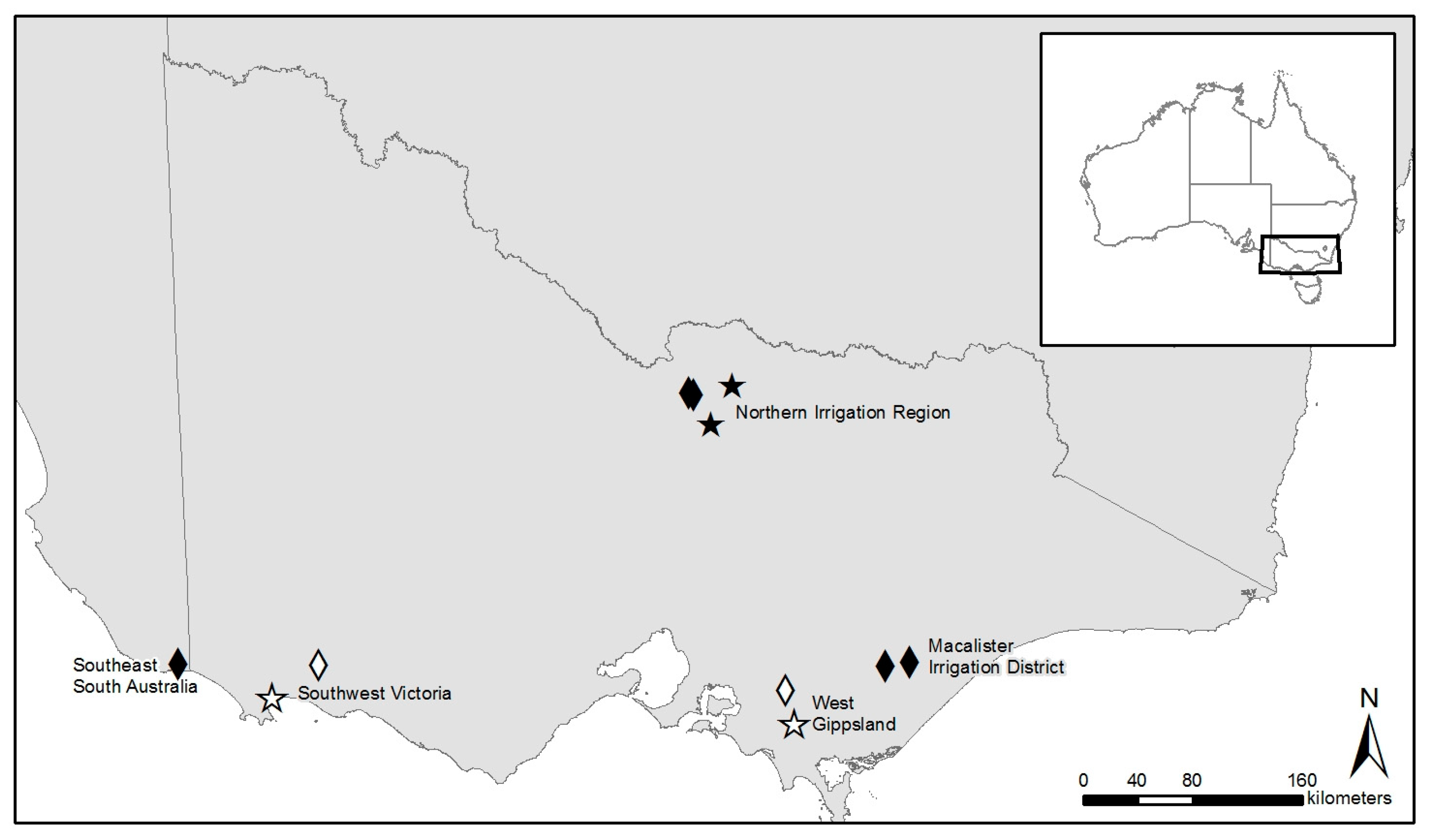
Figure 1. Surveyed farm locations across southeast Australia. Farms, where calibration and validation data were collected, have a diamond symbol, and validation-only farms have a star symbol (open = dryland, filled = irrigated).
Remotesensing 15 02915 g001
Figure 2. Three pasture observations and destructive cuts were taken in each 10 × 10 m sample pixel (sampling unit), and the mean pasture dry matter yield was calculated. The number and the orientation of the pixels across the paddocks depended on paddock size. The minimum sample per paddock was five pixels.
Remotesensing 15 02915 g002
Figure 3. Image selection was based on the calculated mean for each ground collection date compared to the total range measured across that paddock. The closest image within the lag range was chosen, where the ground collection date mean was within +/−1 standard deviation of the paddock mean.
Remotesensing 15 02915 g003
Figure 4. Timescale of image acquisition and ground data collection of this study for (a) calibration and internal validation and (b) independent validation.
Remotesensing 15 02915 g004
Figure 5. Data analysis workflow for the machine learning algorithm development for pasture biomass estimation.
Remotesensing 15 02915 g005
Figure 6. Pearson correlation matrix indicating the strength of relationships between the Band Index (Table 2, column 2). DM stands for dry matter. A dark thin diagonal straight line represents a perfect 1:1 relationship, and as the relationship reduces, the line becomes wider and lighter in colour.
Remotesensing 15 02915 g006
Figure 7. The agreement between the measured and predicted pasture yield obtained from (a) internal validation and (b) independent validation.
Remotesensing 15 02915 g007
Figure 8. The variable importance generated from the best-performing RF model through the Boruta algorithm. Refer to Table 2 for the description of Bands. Season and management are categorical variables and are described in Section 2.6.3.
Remotesensing 15 02915 g008
Figure 9. Demonstration of model accuracy based on two validations in different seasons: (a) internal and (b) independent validations (both dryland and irrigated data combined). Data were not available for all seasons.
Remotesensing 15 02915 g009
Figure 10. All validations based on management (dryland/irrigated): (a) internal and (b) independent across all farms and seasons.
Remotesensing 15 02915 g010
Figure 11. Prediction model results without including SWIR bands and associated SI.
Remotesensing 15 02915 g011
Figure 12. Flowchart for model automation to estimate pasture biomass.
Remotesensing 15 02915 g012
Figure 13. Pasture biomass prediction image (kg DM/ha) in 2019 and 2020 for PS04 farms across different seasons: (a) July (winter), (b) September (early spring), (c) October (late spring), (d) December (summer), and (e) April (autumn).
Remotesensing 15 02915 g013
Table 1. Characteristics of each farm in this study. Data from the first seven farms were used to calibrate and validate the model. Data from PS11, PS19, PS28, and PS31 provided independent validation.
FarmRegionAnnual Median Rainfall (mm)Annual Median Temperature Range (°C)Predominant Australian Soil OrderIrrigated/DrylandFarm Size (ha)Average Paddock Size (ha)
PS01Macalister Irrigation District5948.2–19.7Chromosol (brown) [52]Irrigated3485.4
PS02Macalister Irrigation District5948.2–19.7Sodosol (brown) [52]Irrigated4106.4
PS03Northern Irrigation Region4378.7–21.8Sodosol (red) [52]Irrigated722.3
PS04Northern Irrigation Region4378.7–21.8Sodosol (red) [52]Irrigated1961.2
PS05Southeast South Australia7678.3–19.1Tenosol [53]Irrigated47115.7
PS06Southwest Victoria7507.8–19.2Dermosol (brown) [52]Dryland3585.3
PS07West Gippsland10019.0–19.7Hydrosol (redoxic), Ferrosol (red) [52]Dryland2311.6
PS11Southwest Victoria7799.4–18.0Chromosol (brown) [52]Dryland3804.5
PS19West Gippsland9758.5–18.7Ferrosol (red) [52]Dryland1152.2
PS28Northern Irrigation Region4869.4–21.9Sodosol (brown) [52]Irrigated3381.7
PS31Northern Irrigation Region5278.7–21.2Sodosol (red) [52]Irrigated9701.9
Table 2. Information on the spectral indices reviewed in rows one to 54, E = Exploratory band combination, V = variation on a published spectral index. Information on original S2 bands used for the prediction model [61], in rows 55 to 66, G = Green, RE = Red Edge, NIR = Near Infrared, R = Red, BL = Blue. The final image stack index list of 21 bands is provided in column two.
Row No.Image IndexName/DescriptionSI Formulae or Original Band InformationSource (If Applicable)
1 Anthocyanin Ref 1(1/B3 G) − (1/B5 RE)[62]
2 Anthocyanin Ref 2B8 NIR × (1/B3 G) − (1/B5 RE)[62]
3 Atmospherically Resistant VegB8A RE − (B4 R − 1 × (B2 Bl − B4 R))/B8A RE − (B4 R − 1 × (B2 BL − B4 R))[63]
4 B11 SWIR/B12 SWIRB11 SWIR/B12 SWIRE
5 B12 SWIR/B11 SWIRB12 SWIR/B11 SWIRE
6Band_1Difference Vegetation Index (DVI)B8 NIR−B4 R[40]
7 Enhanced Vegetation Index (EVI)2.5 × ((B8A RE − B4 R)/(B8A RE + 6 × B4 R − 7.5 × B2 BL + 1))[64]
8Band_2EVI 22.5 × (B8 NIR − B4 R)/(B8 NIR + 2.4) × (B4 R + 1)[65]
9 B11 SWIR/B8 NIRB11 SWIR/B8 NIRE
10 B11 SWIR/B8A NIRB11 SWIR/B8A NIRE
11 B12 SWIR/B8 NIRB12 SWIR/B8 NIRE
12Band_3B12 SWIR/B8A NIRB12 SWIR/B8A NIRE
13Band_4Global Environmental Monitoring Index(2 × ((B8 NIR × B8 NIR) − (B4 R × B4 R)) + (1.5 × B8 NIR + 0.5 × B4 R)/(B8 NIR + B4 R + 0.5)) × (1 − 0.25 × (2 × ((B8 NIR × B8 NIR) − (B4 R × B4 R)) + (1.5 × B8 NIR + 0.5 × B4 R)/(B8 NIR + B4 R + 0.5))) − (B4 R − 0.125)/(1 − B4 R)[66]
14 Green Atmospherically Resistant Index(B8 NIR − (B3 G − 1.7 × (B2 BL − B4 R)))/(B8 NIR + (B3 G − 1.7 × (B2 BL − B4 R)))[67]
15 Green Chlorophyll Index (B8)B8 NIR[68]
16 Green Chlorophyll Index (B8A)B8A NIR[68]
17Band_5Green Difference Vegetation Index (B8)B8 NIR − B3 G[69]
18 Green Difference Index (B8A)B8A NIR − B3 GV
19Band_6Green Leaf index (GLI)((B3 G − B4 R) + (B3 G − B2 BL))/(B3 G + B4 R + B3 G + B2 BL)[70]
20 Green NDVI(B8 NIR − B3 G)/(B8 NIR + B3 G)[71]
21 B8 NIR/B3 GreenB8 NIR/B3 GE
22 B8A NIR/B3 GreenB8A NIR/B3 GE
23Band_7Leaf Area Index (LAI) from EVI3.618 × (2.5 × (B8 NIR − B4 R)/1 + B8 NIR + (6 × B4 R) − (7.5 × B2 BL)) − 0.118[72]
24 Modified Chlorophyll Absorption Ratio((B5 RE − B4 R) − 0.2 × (B5 RE − B3 G)) × (B5 RE/B4 R)[73]
25 Modified Chlorophyll Abs Ratio IMPROVED(1.5 × (2.5 × (B7 RE-B4 R)) − 1.3 × (B7 RE − B3 G))/sqrt((2 × B7 RE + 1) × (2 × B7 RE + 1)) − (6 × B7 RE − 5 × sqrt(B4 R) − 0.5)[74]
26 Modified Red Edge NDVI(B6 RE − B5 RE)/(B6 RE + B5 RE − 2 × B2 BL)[75]
27 Modified Red Edge Simple Ratio(B6 RE − B2 BL)/(B5 RE − B2 BL)[75,76]
28 Modified simple ratio((B8 NIR/B4 R) − 1)/((sqrt((B8 NIR/B4 R))) + 1)[77]
29 M SAVI 2(2 × B8 NIR + 1 − sqrt((2 × B8 NIR + 1) × (2 × B8 NIR + 1) − 8 × (B8 NIR − B4 R)))/2[78]
30 Modified Triangular Veg Index1.2 × (1.2 × (B7 RE − B3 G) − 2.5 × (B4 R − B3 G))[74]
31 Modified Triangular VI IMPROVED(1.5 × (2.5 × (B7 RE − B4 R)) − 1.3 × (B7 RE − B3 G))/sqrt((2 × B7 RE + 1) × (2 × B7 RE + 1)) − (6 × B7 RE − 5 × sqrt(B4 R) − 0.5)[74]
32 Non-linear Index((B8 NIR × B8 NIR) − B4 R)/((B8 NIR × B8 NIR) + B4 R)[79]
33 Normalised Difference Vegetation Index (NDVI)(B8 NIR − B4 R)/(B8 NIR + B4 R)[13]
34 Optimised Soil Adjusted Vegetation Index (OSAVI)(B8A RE − B4 R)/(B8A RE + B4 R + 0.16)[80]
35 Plant Senescence Reflectance index(B4 R − B2 BL)/B6 RE[81]
36Band_8Red Edge NDVI(B6 RE − B5 RE)/(B6 RE + B5 RE)[76]
37 Renormalised Difference Vegetation Index(B8 NIR − B4 R)/sqrt(B8 NIR + B4 R)[82]
38 B8 NIR/B4 RedB8 NIR/B4 RE
39 B8A NIR/B4 RedB8A NIR/B4 RE
40 Soil Adjusted Vegetation Index (SAVI)((B8 NIR − B4 R)/(B8 NIR + B4 R + 0.5)) × 1.5[83]
41 Structure Insensitive Pigment IndexB7 RE − B2 BL/B7 RE − B4 R[84]
42 Transformed Difference Veg Index1.5 × ((B8 NIR − B4 R)/(sqrt(B8 NIR × B8 NIR) + B4 R + 0.5))[85]
43 Triangular Greenness Index(−0.5 × ((665 − 492) × (B4 R − B3 G) − (665 − 492) × (B4 R − B2 BL))[86]
44 Triangular Vegetation Index(120 × (B6 RE − B3 G) − 200 × (B4 R − B3 G))/2[42]
45 Visible Atmospherically Resistant Index(B3 G − B4 R)/(B3 G + B4 R − B2 BL)[62]
46 Wide Dynamic Range Veg Index(0.2 × B8 NIR − B4 R)/(0.2 × B8 NIR + B4 R)[87,88]
47 Red Edge(B5) Simple Ratio IndexB8 NIR/B5 RE[89]
48Band_9Red Edge(B6) Simple Ratio IndexB8 NIR/B6 REV
49 Red Edge(B7) Simple Ratio IndexB8 NIR/B7 REV
50 Red Edge(8A) Simple Ratio IndexB8 NIR/B8A NIRV
51 Red Edge(B5) Chlorophyll Index(B8 NIR/B5 RE) − 1[90]
52 Red Edge(B6) Chlorophyll Index(B8 NIR/B6 RE) − 1V
53 Red Edge(B7) Chlorophyll Index(B8 NIR/B7 RE) − 1V
54 Red Edge(B8A) Chlorophyll Index(B8 NIR/B8A NIR) − 1V
Original S2 BandsS2A, S2B band centre/S2A, S2B band width/resolution
55Band_10B1 Aerosols442.7, 442.2/21, 21/60
56Band_11B2 Blue492.4, 492.1/66, 66/10
57Band_12B3 Green559.8, 559.0/36, 36/10
58Band_13B4 Red664.6, 664.9/31, 31/10
59Band_14B5 Red Edge704.1, 703.8/15, 16/20
60Band_15B6 Red Edge740.5, 739.1/15, 15/20
61Band_16B7 Red Edge782.8, 779.7/20, 20/20
62Band_17B8 NIR832.8, 832.9/106, 106/10
63Band_18B8A NIR864.7, 864.0/21, 22/20
64Band_19B9 Water Vapour945.1, 943.2/20, 21/60
65Band_20B11 SWIR 11613.7, 1610.4/91, 94/20
66Band_21B12 SWIR 22202.4, 2185.7/175, 185/20
Table 3. Data, sample size, and model accuracy for internal and independent validations.
Model Accuracy Indicators
TypeField Data (kg DM/ha)Model Development DataShapiro-Wilk TestRandom Forest Model
MinMaxCalibrationValidationw-Valuep-ValueR2LCCCRMSE (kg DM/ha)NRMSE
Internal
validation
6685777171430.9596<0.050.900.72439.4915.08
Independent validation4114838 840.9571<0.050.880.68457.0519.83
Table 4. A comparison of model accuracy and efficiency with and without SWIR bands. The results are from PS04 farm during a day from the summer season.
Accuracy and Efficiency IndicatorsR2LCCCRMSE (kg DM/ha)NRMSEMaximum Biomass Predicted (kg DM/ha)
With SWIR bands0.900.72439.4915.084348.25
Without SWIR bands0.790.57635.4621.803379.62
Disclaimer/Publisher’s Note: The statements, opinions and data contained in all publications are solely those of the individual author(s) and contributor(s) and not of MDPI and/or the editor(s). MDPI and/or the editor(s) disclaim responsibility for any injury to people or property resulting from any ideas, methods, instructions or products referred to in the content.