
Analytical Modeling of Electromagnetic Scattering and HRRP Characteristics from the 3D Sea Surface with a Plunging Breaker


Abstract

1. Introduction
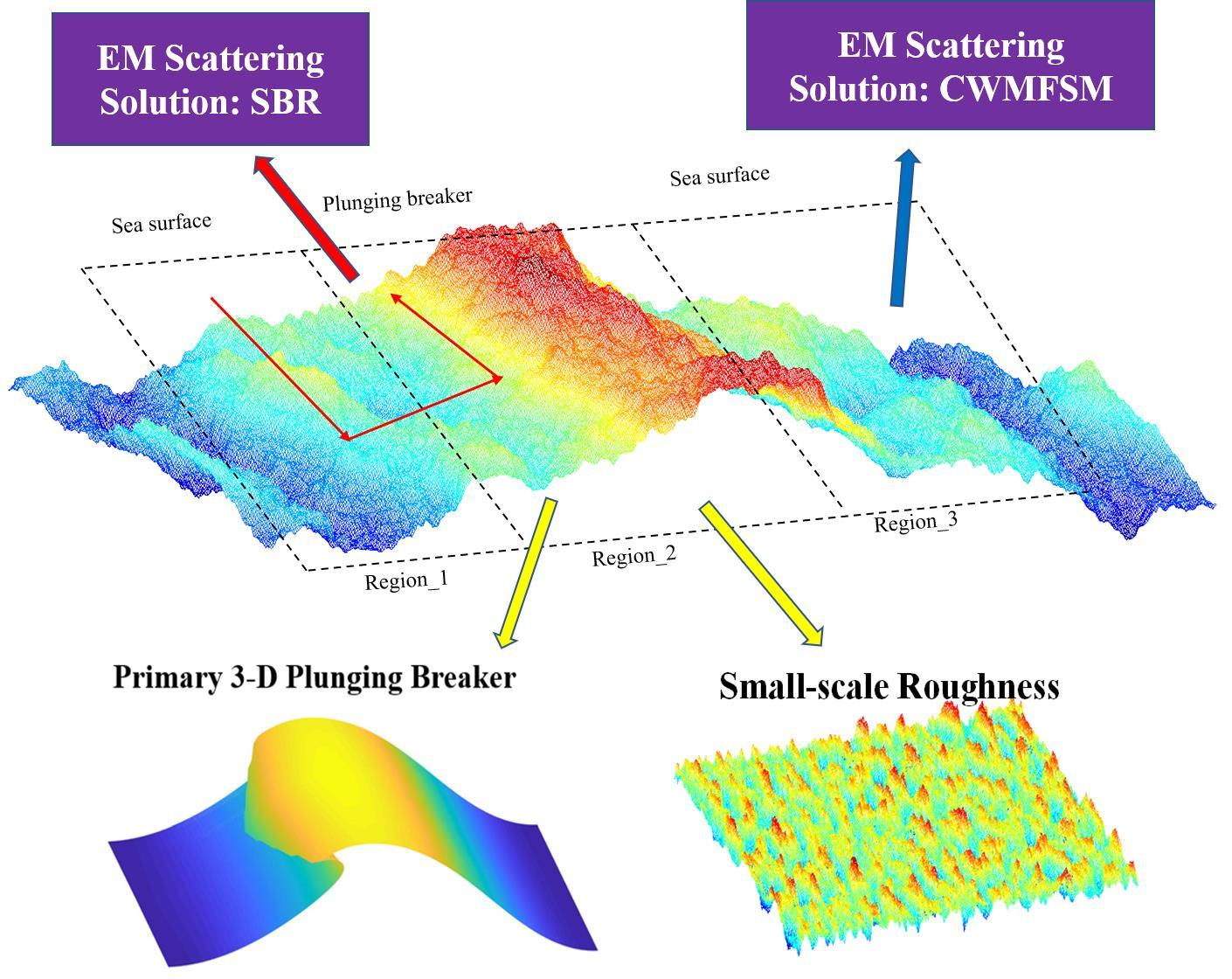
2. EM Scattering Modeling of the 3D Sea Surface with a Plunging Breaker
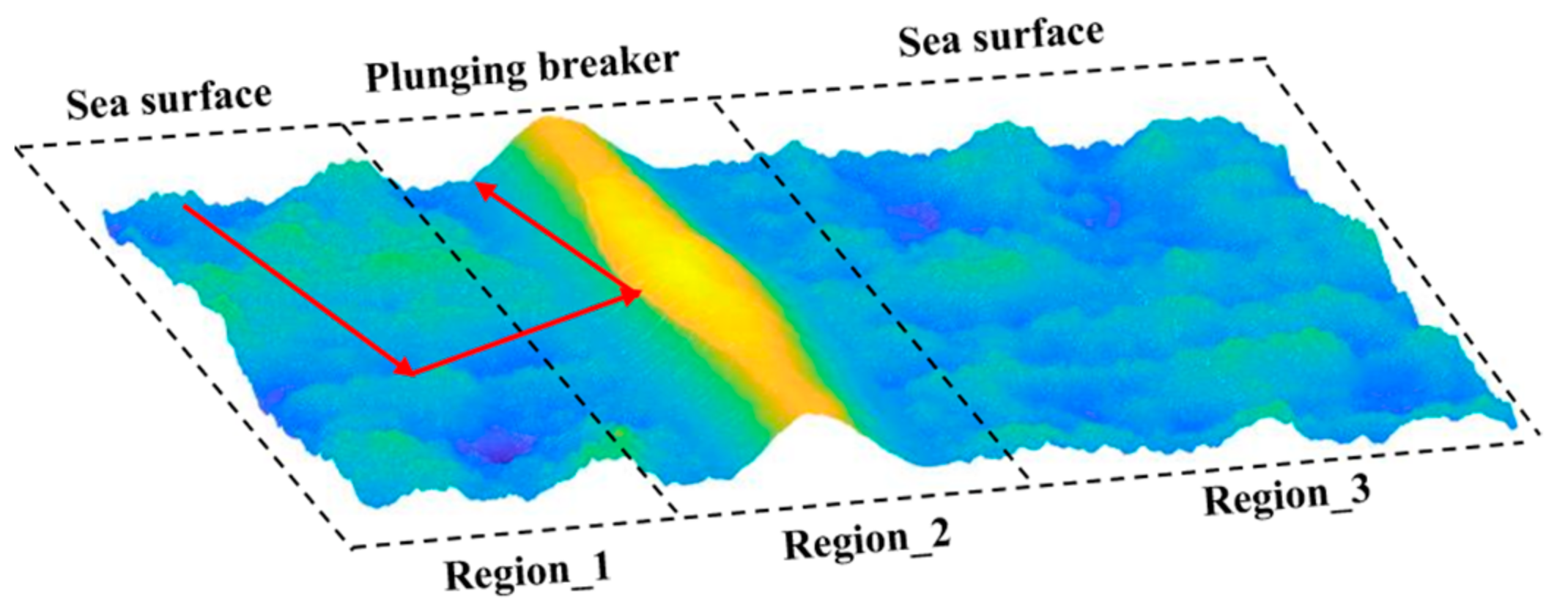
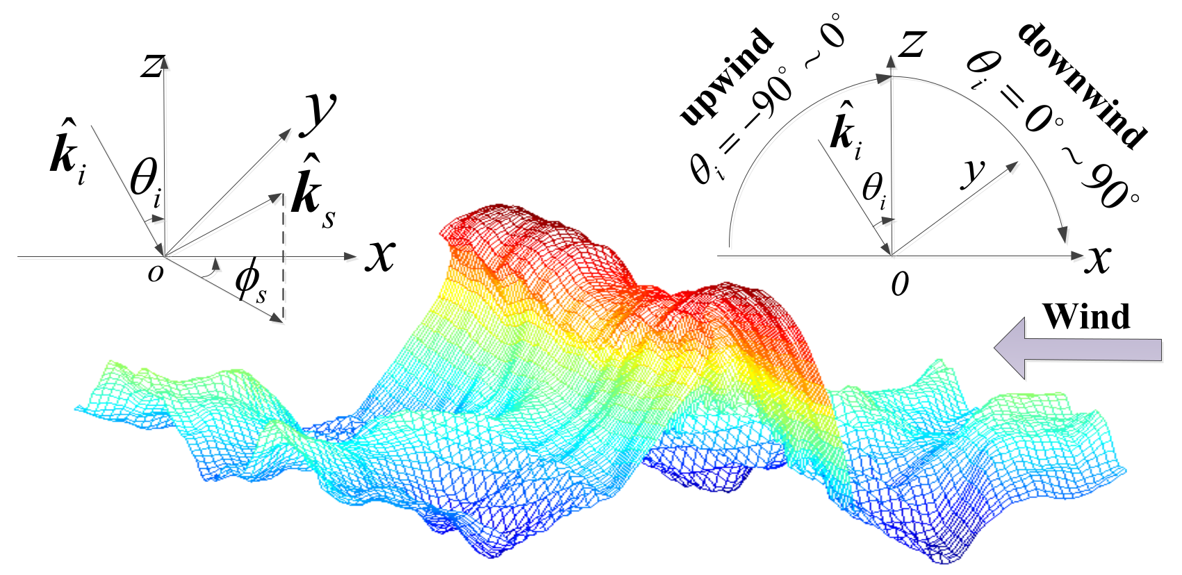
2.1. Geometric Modeling of the 3D Sea Surface with a Plunging Breaker
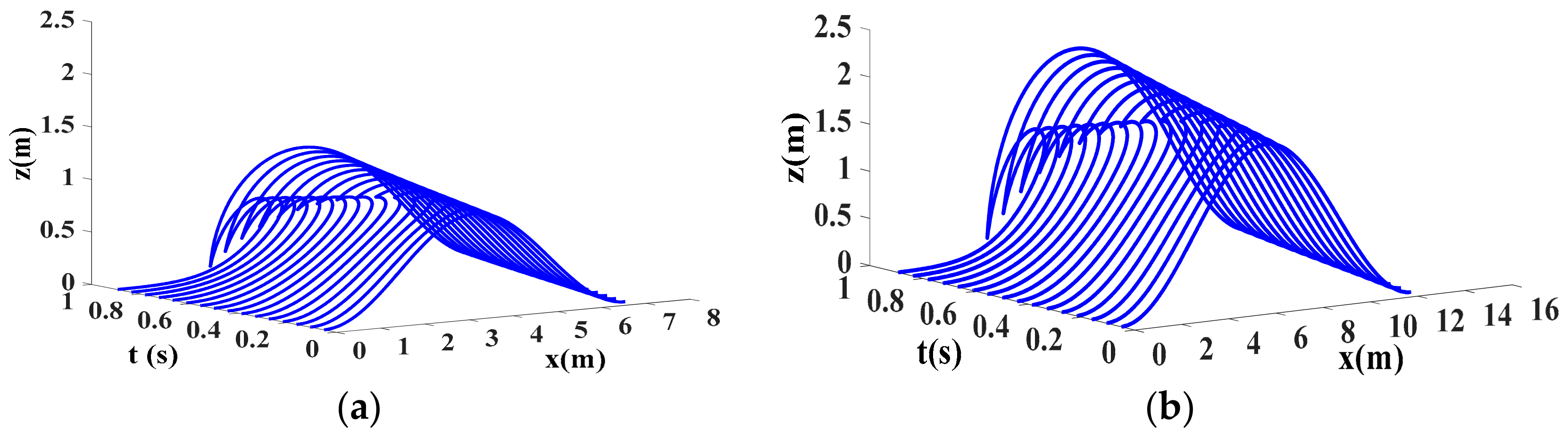
2.1.1. Construction of the Primary 3D Plunging Breaker
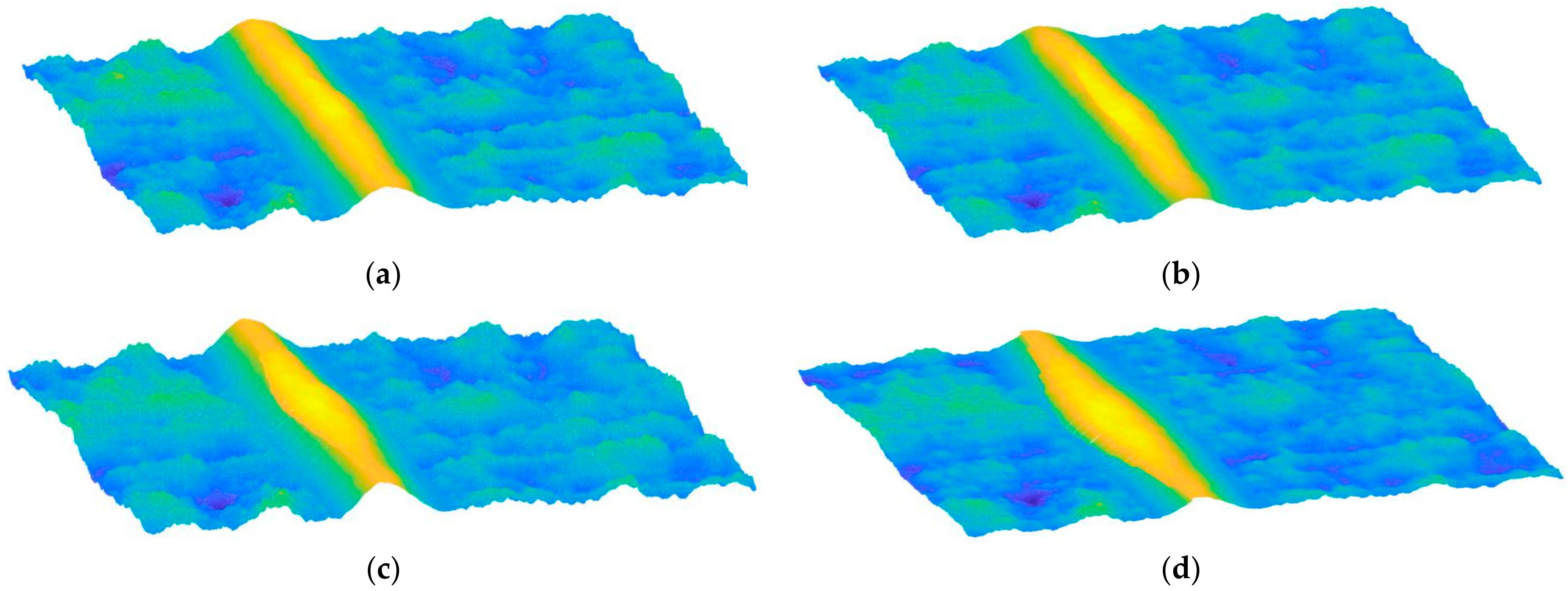
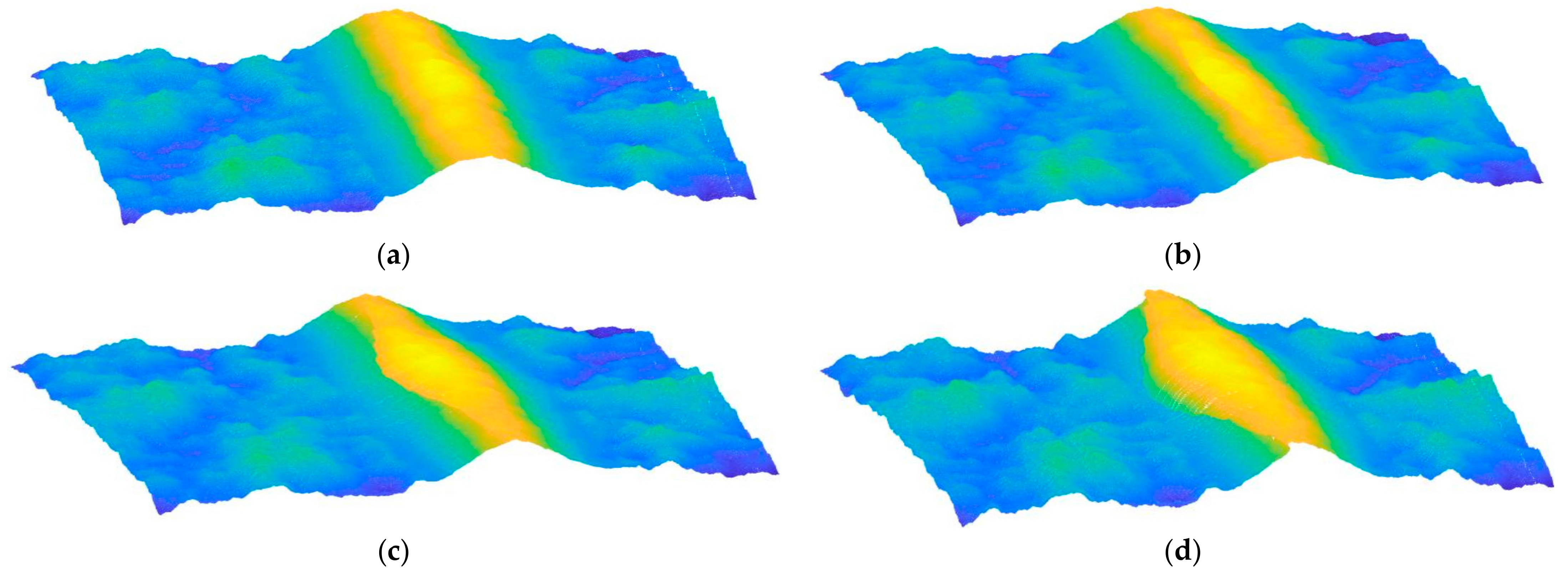
2.1.2. Construction of the 3D Sea Surface with a Plunging Breaker
2.2. EM Scattering Modeling of the 3D Sea Surface with a Plunging Breaker
2.2.1. CWMFSM
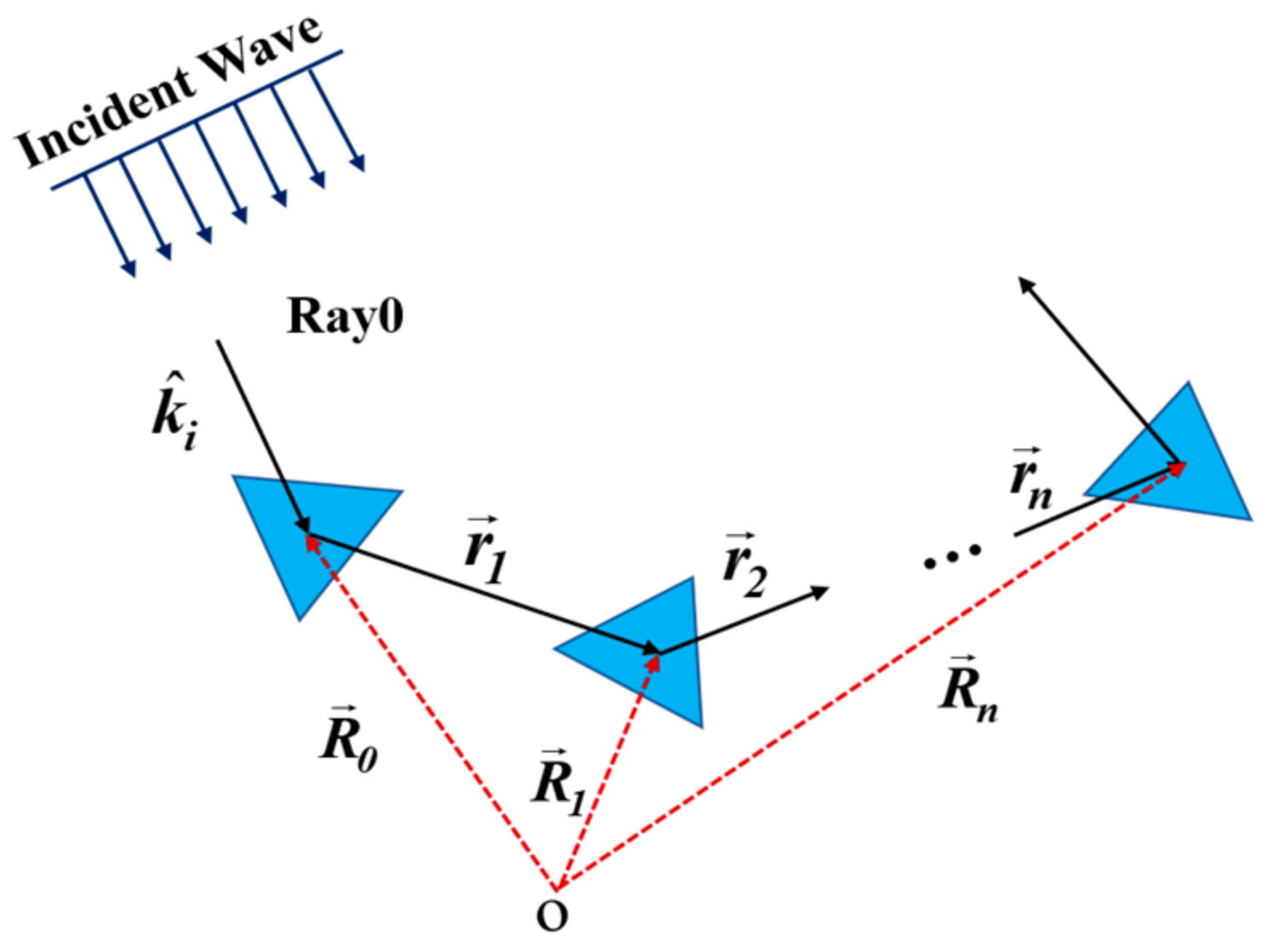
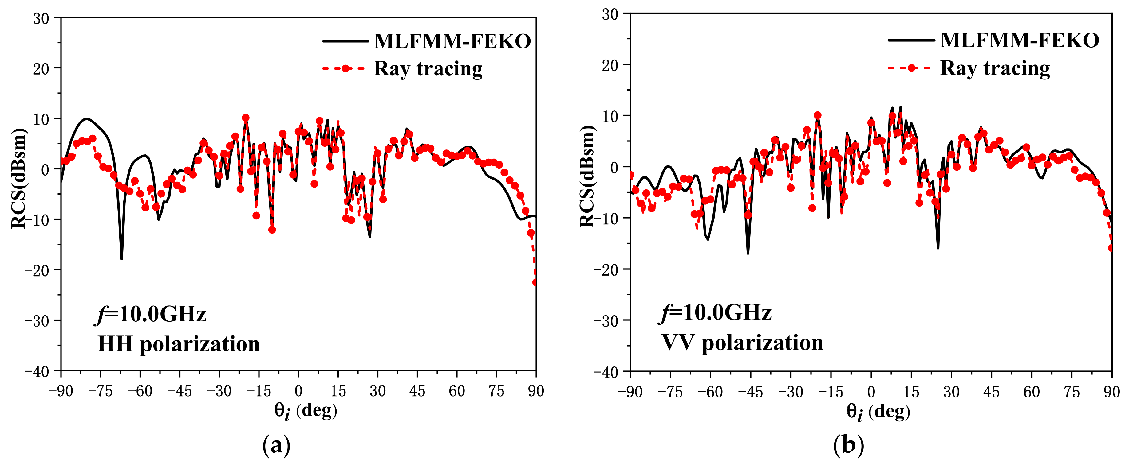
2.2.2. Ray Tracing Technique
3. Results
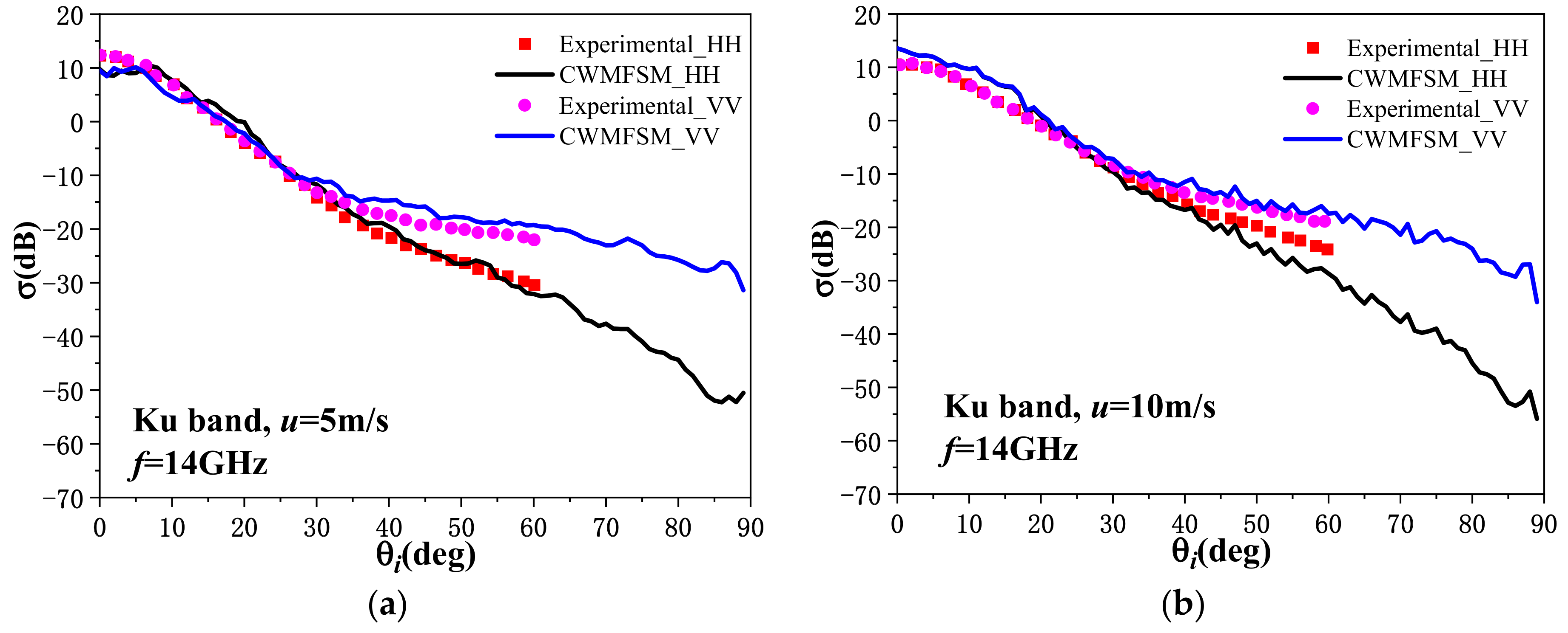
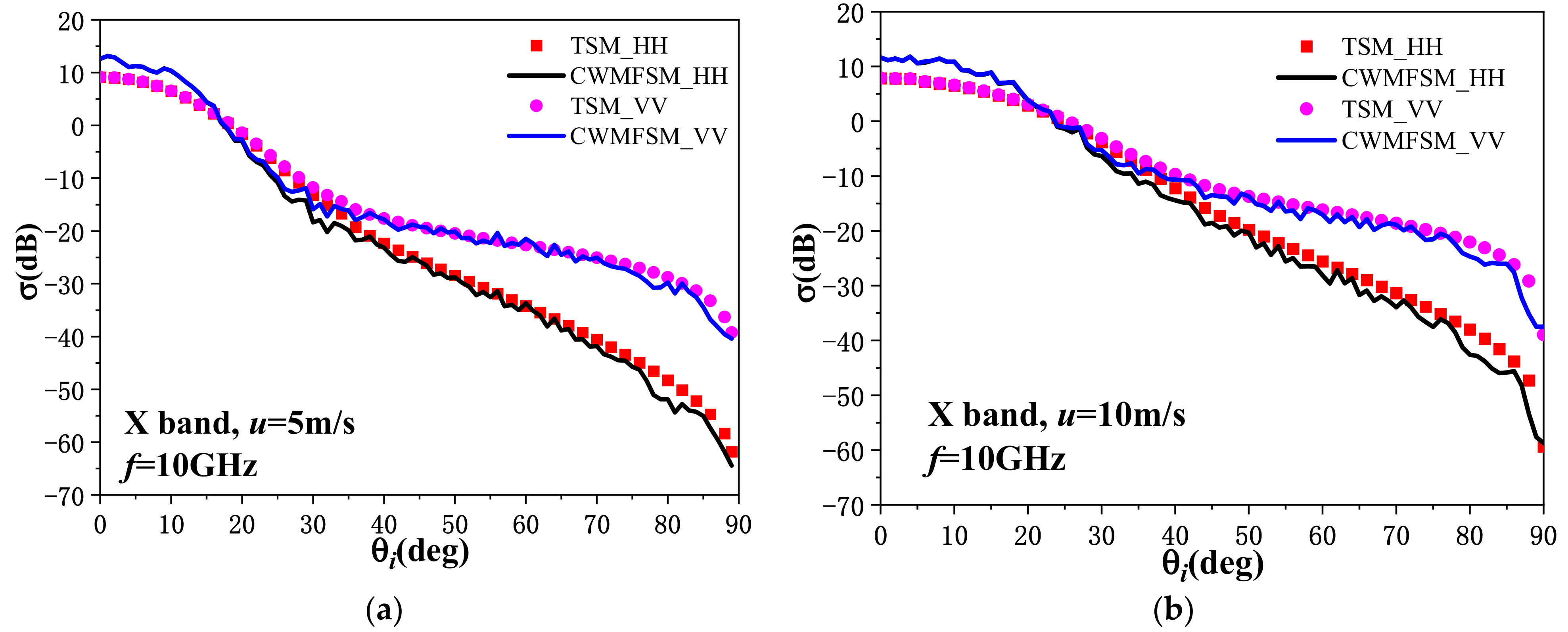
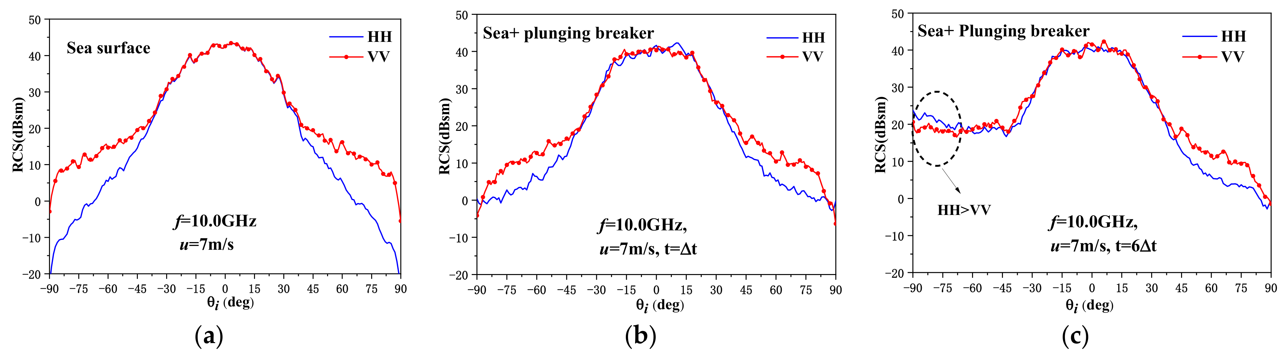
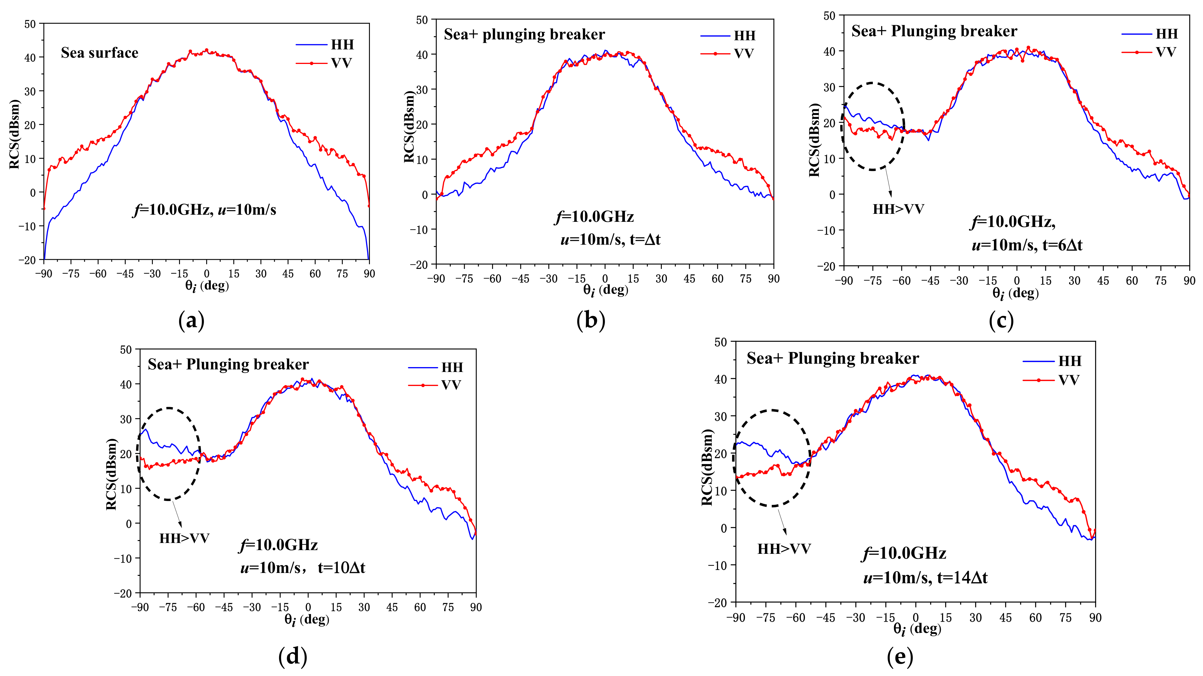
3.1. Backscattering Radar Cross Section
3.2. Spatial Distribution of the Backscattering Electric Field
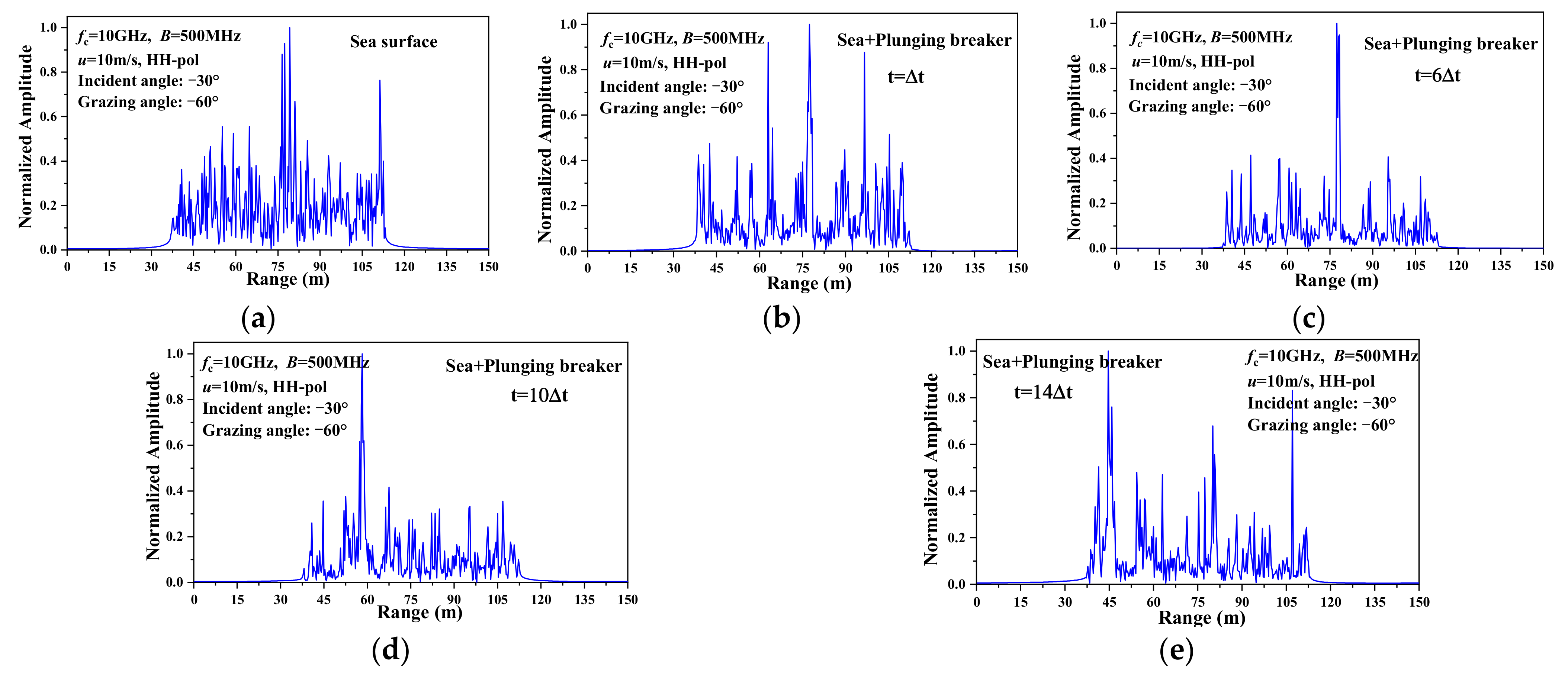
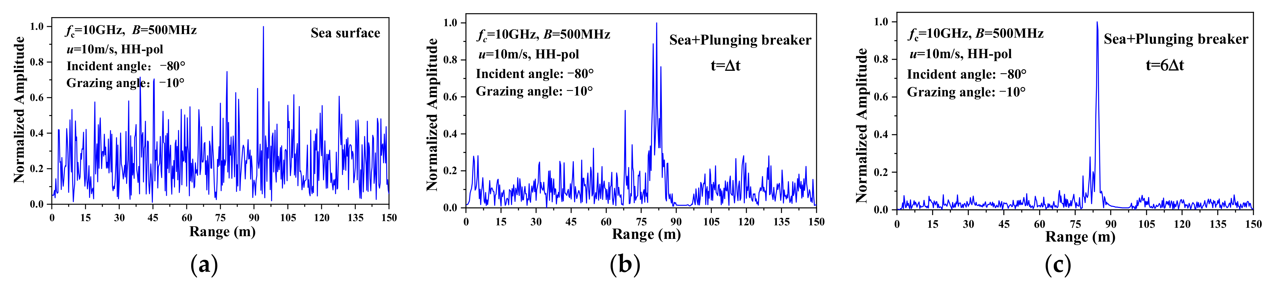
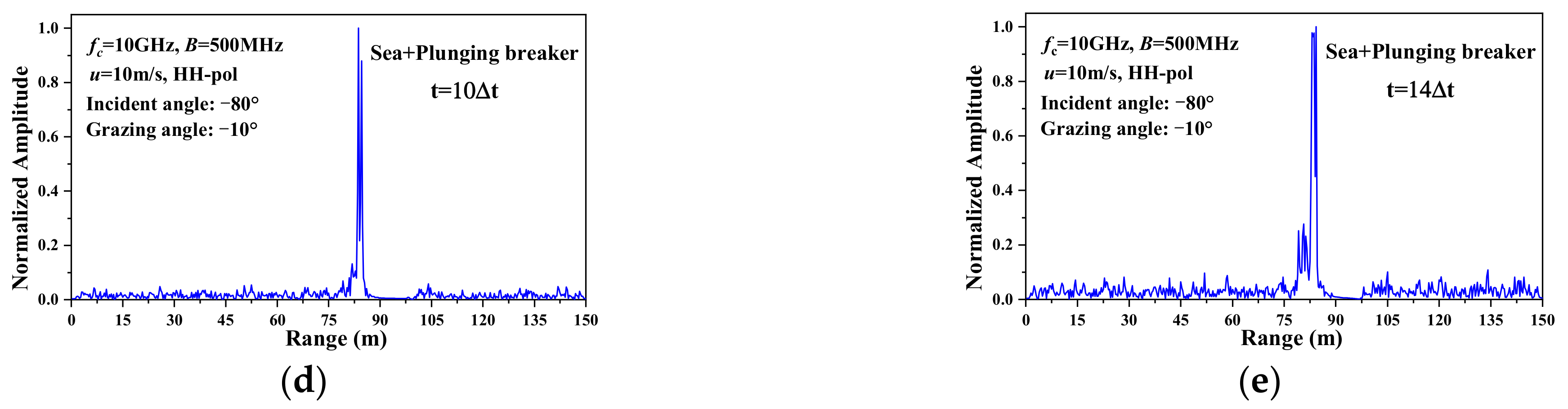
3.3. HRRP of the 3D Sea Surface with a Plunging Breaker
4. Conclusions
- (1)
- The plunging breaker is one of the main reasons for the sea-spike phenomenon, which appears to be more obvious during the generation process of a plunging breaker. In addition, the profile of a plunging breaker has a significant effect on the scattering results.
- (2)
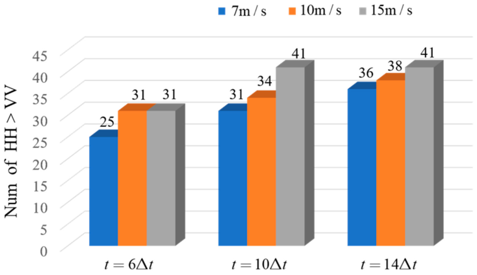
- The backscattering RCS varies more dramatically for the upwind incidence than for the downwind incidence when there exists a plunging breaker. Meanwhile, the sea-spike phenomenon is more likely to occur for a large incident angle, upwind incidence, and a high wind speed.
- (3)
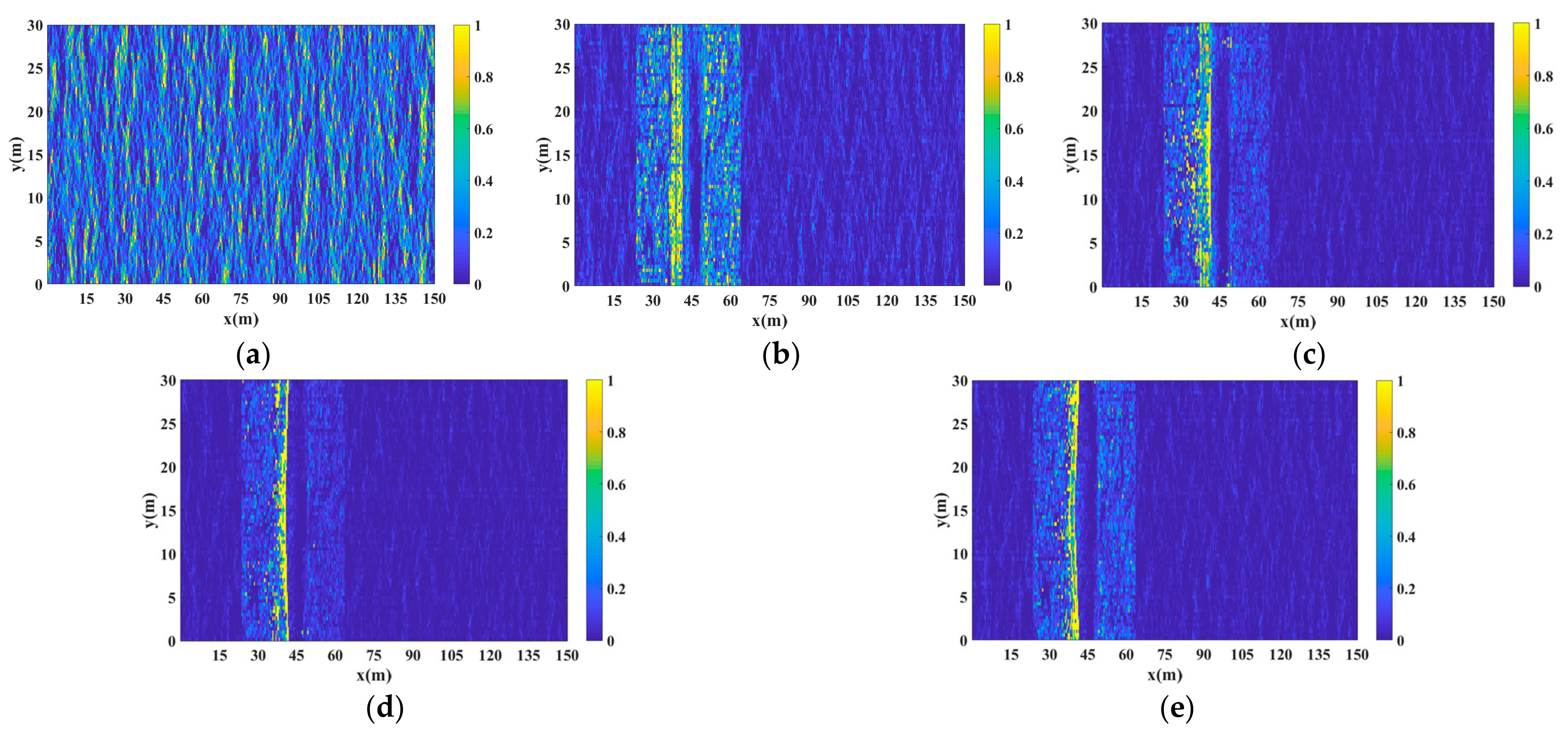
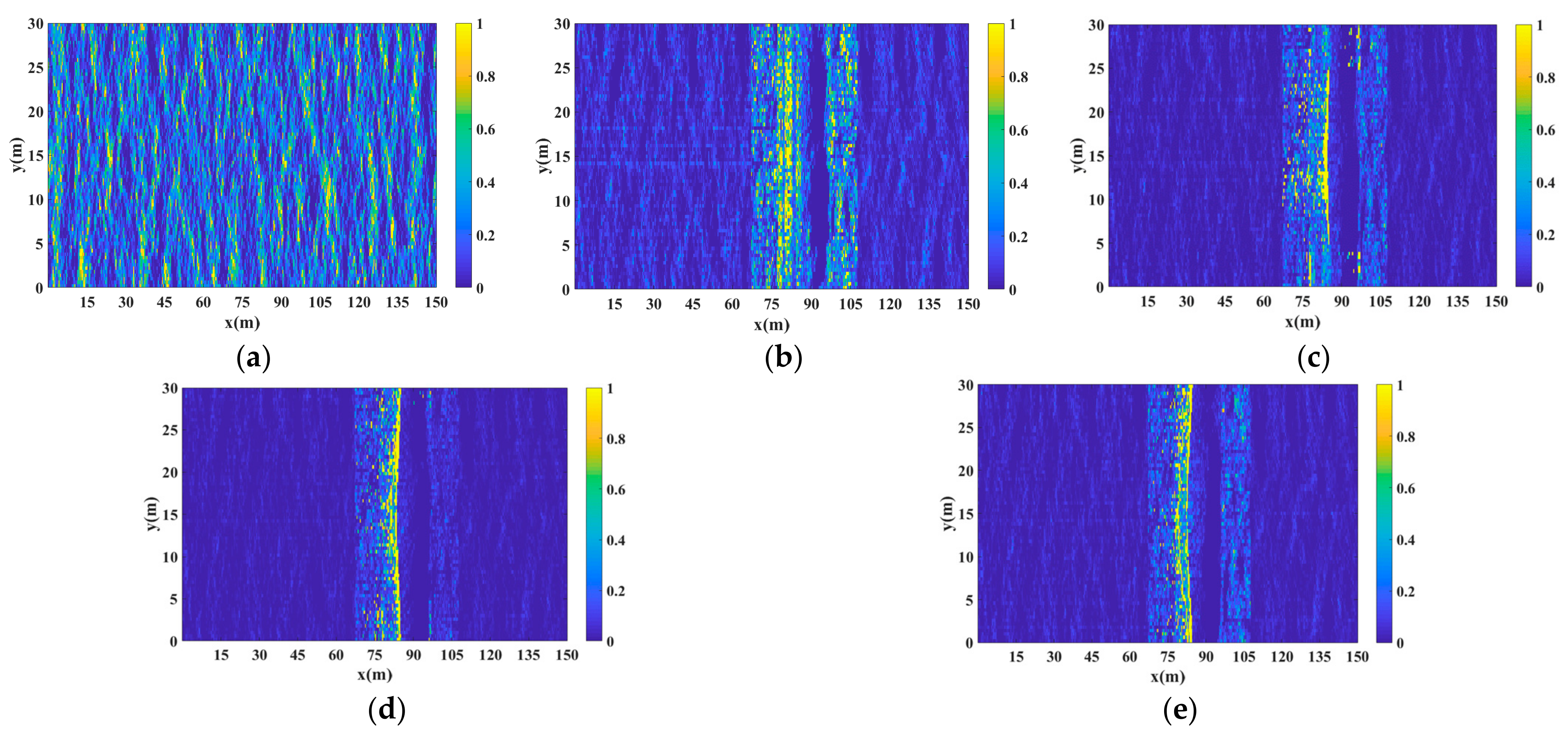
- The amplitude of the backscattering electric field from the plunging breaker region is much stronger than that of the sea surface and increases with wind speed. It exhibits sharp and short bursts in the sea background clutter.
- (4)
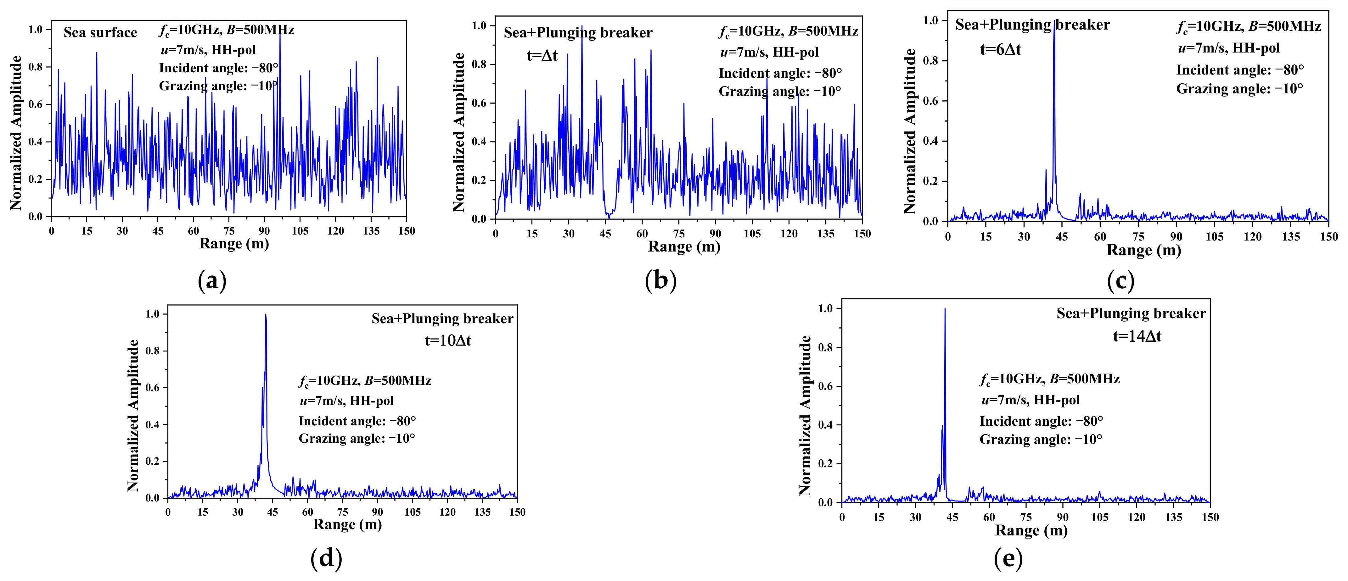
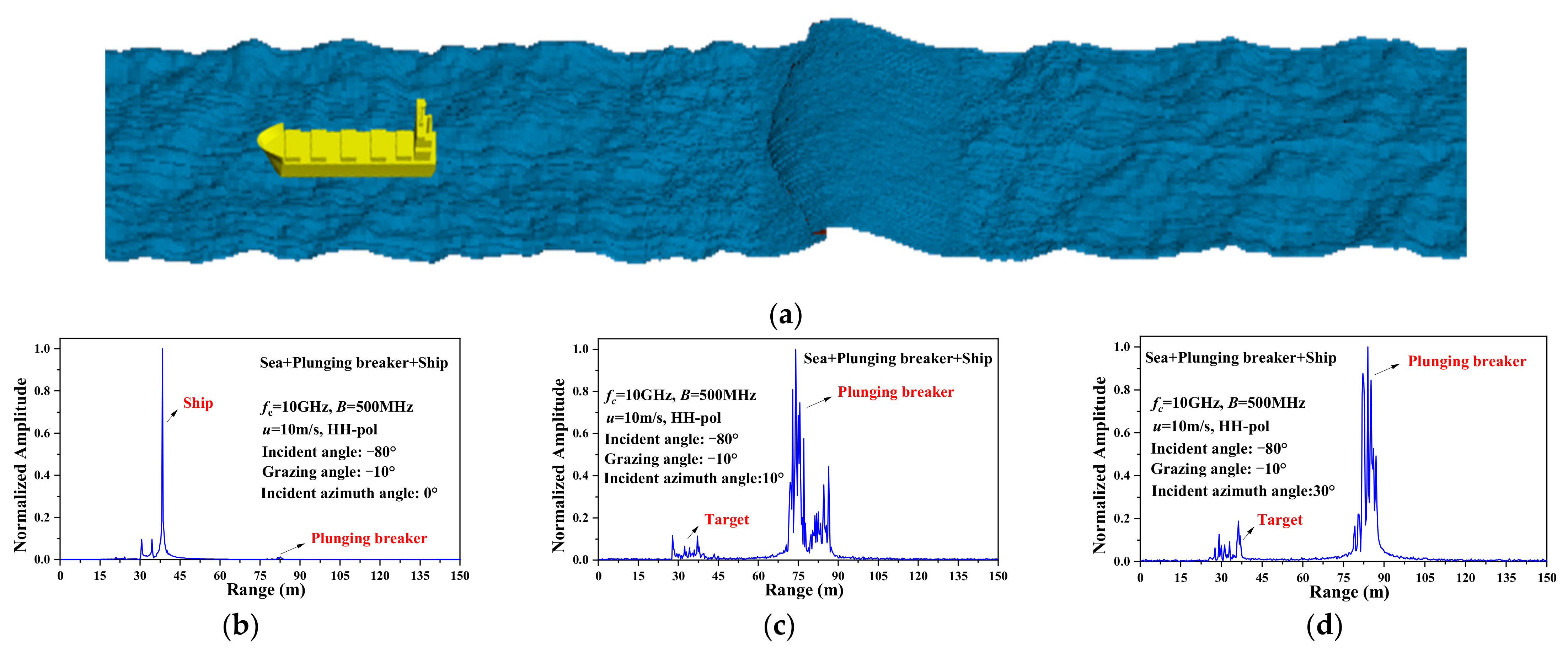
- For the upwind and large incident angle, noticeable sharp peaks occurred in the HRRP of 3D sea surface with a plunging breaker when the steep crest of the plunging breaker is generated. Moreover, the location of the peak coincides with the crest of the plunging breaker.
- (5)
- A target-like feature is shown in the HRRP of the 3D sea surface with a plunging breaker, which will have a great influence on target detection and recognition.
Author Contributions
Funding
Conflicts of Interest
References
- Ulaby, F.T.; Moore, R.K.; Fung, A.K. Microwave Remote Sensing: Active and Passive: Radar Remote Sensing and Surface Scattering and Emission Theory; Addison Wesley: Hoboken, NJ, USA, 1982. [Google Scholar]
- Bass, F.G.; Fuks, I.M.; Kalmykov, A.I. Very high frequency radiowave scattering by a disturbed sea surface Part I: Scattering from a slightly disturbed boundary. IEEE Trans. Antennas Propag. 1968, 16, 554–559. [Google Scholar] [CrossRef]
- Bass, F.G.; Fuks, I.M.; Kalmykov, A.I. Very high frequency radiowave scattering by a disturbed sea surface Part II: Scattering from an actual sea surface. IEEE Trans. Antennas Propag. 1968, 16, 560–568. [Google Scholar] [CrossRef]
- Qiao, T.; Tsang, L.; Vandemark, D. Sea Surface Radar Scattering at L-Band Based on Numerical Solution of Maxwell’s Equations in 3-D (NMM3D). IEEE Trans. Geosci. Remote Sens. 2018, 56, 3137–3147. [Google Scholar] [CrossRef]
- Melief, H.W.; Greidanus, H.; Genderen, P.V. Analysis of sea spikes in radar sea clutter data. IEEE Geosci. Remote Sen. Lett. 2006, 44, 985–993. [Google Scholar] [CrossRef]
- Posner, F.; Gerlach, K. Sea spike demographics at high range resolutions and very low grazing angles. In Proceedings of the 2003 IEEE Radar Conference, Huntsville, AL, USA, 8 May 2003. [Google Scholar]
- Smith, M.J.; Poulter, E.M.; McGregor, J.A. Doppler radar measurements of wave groups and breaking waves. J. Geophys Res. 1996, 101, 14269–14282. [Google Scholar] [CrossRef]
- Rosenberg, L. Sea-spike detection in high grazing angle X-band sea-clutter. IEEE Trans. Geosci. Remote Sens. 2013, 51, 4556–4562. [Google Scholar] [CrossRef]
- Rino, C.L.; Ngo, H.D. Numerical simulation of low-grazing-angle ocean microwave backscatter and its relation to sea spikes. IEEE Trans. Antennas Propag. 1998, 46, 133–141. [Google Scholar] [CrossRef]
- Sletten, M.A.; West, J.C.; Liu, X.; Duncan, J.H. Radar investigations of breaking water at low grazing angles with simultaneous high-speed optical imagery. Radio Sci. 2003, 38, 18-1–18-17. [Google Scholar] [CrossRef]
- Wang, P.; Yao, Y.; Tulin, M.P. An efficient numerical tank for nonlinear water waves, based on the multi-subdomain approach with BEM. Int. J. Numer. Methods Fluids 1995, 20, 1315–1336. [Google Scholar] [CrossRef]
- Holliday, D.; Deraad, L. Sea-spike backscatter from a steepening wave. IEEE Trans. Antennas Propag. 1998, 46, 108–113. [Google Scholar] [CrossRef]
- West, J.C. Low-grazing-angle (LGA) sea-spike backscattering from plunging breaker crests. IEEE Trans. Geosci. Remote Sens. 2002, 40, 523–526. [Google Scholar] [CrossRef]
- West, J.C.; Ja, S.J.; Duncan, J.H.; Qiao, H. LGA scattering from breaking water waves-further results. In Proceedings of the IEEE 1999 International Geoscience and Remote Sensing Symposium, Hamburg, Germany, 28 June–2 July 1999. [Google Scholar]
- West, J.C. Ray analysis of low-grazing scattering from a breaking water wave. IEEE Trans. Geosci. Remote Sens. 1999, 37, 2725–2727. [Google Scholar] [CrossRef]
- Zhao, Z.Q.; West, J.C. Extended GO modeling of microwave backscattering from measured breaking wave crests. In Proceedings of the 2003 IEEE International Geoscience and Remote Sensing Symposium, Toulouse, France, 21–25 July 2003. [Google Scholar]
- West, J.C.; Zhao, Z.Q. Electromagnetic modeling of multipath scattering from breaking water waves with rough faces. IEEE Trans. Geosci. Remote Sens. 2002, 40, 583–592. [Google Scholar] [CrossRef]
- West, J.C.; Sturm, M.J.; Ja, S.J. Low-grazing scattering from breaking water waves using an impedance boundary MM/GTD approach. IEEE Trans. Antennas Propag. 1998, 46, 93–100. [Google Scholar] [CrossRef]
- Yang, W.; Zhao, Z.; Qi, C.; Nie, Z. Electromagnetic modeling of breaking waves at low grazing angles with adaptive higher order hierarchical legendre basis functions. IEEE Trans. Geosci. Remote Sens. 2011, 49, 346–352. [Google Scholar] [CrossRef]
- Li, Y.Z.; West, J.C. Microwave scattering from 3-D breaking water wave crests. In Proceedings of the 2004 IEEE International Geoscience and Remote Sensing Symposium, Anchorage, AK, USA, 20–24 September 2004. [Google Scholar]
- Li, Y.Z.; West, J.C. Low-grazing-angle scattering from 3-D breaking water wave crests. IEEE Trans. Geosci. Remote Sens. 2006, 44, 2093–2101. [Google Scholar]
- Zhao, Z.Q.; West, J.C. Low grazing angle microwave scattering from a three-dimensional spilling breaker crest: A numerical investigation. IEEE Trans. Geosci. Remote Sens. 2005, 43, 286–294. [Google Scholar] [CrossRef]
- Zhao, Z.Q.; West, J.C. Two-scale analysis of LGA scattering from a 3-D spilling breaker crest. In Proceedings of the IEEE Antennas and Propagation Society International Symposium, Columbus, OH, USA, 22–27 June 2003. [Google Scholar]
- Jeschke, S.; Birkholz, H.; Schumann, H. A Procedural Model for Interactive Animation of Breaking Ocean Waves; UNION Agency Science Press: Plzen, Czech Republic, 2003; Volume 14, pp. 17–20. [Google Scholar]
- Zhang, M.; Chen, H.; Yin, H.C. Facet-based investigation on EM scattering from electrically large sea surface with two-scale profiles: Theoretical model. IEEE Trans. Geosci. Remote Sens. 2011, 49, 1967–1975. [Google Scholar] [CrossRef]
- Li, W.L.; Guo, L.X.; Meng, X.; Liu, W. Modeling and electromagnetic scattering from the overturning wave crest. Acta Phys. Sin. 2014, 63, 164102. [Google Scholar]
- Elfouhaily, T.; Chapron, B.; Katsaros, K.; Vandemark, D. A unified directional spectrum for long and short wind-driven waves. J. Geoph Res. 1997, 102, 15781–15796. [Google Scholar] [CrossRef]
- Voronovich, A.G.; Zavorotny, V.U. Theoretical model for scattering radar signals in Ku- and C-bands from a rough sea surface with breaking wave. Waves Random Media 2001, 11, 247–269. [Google Scholar] [CrossRef]
- Meissner, T.; Wentz, F.J. The complex dielectric constant of pure and sea water from microwave satellite observations. IEEE Trans. Geosci. Remote Sens. 2004, 42, 1836–1849. [Google Scholar] [CrossRef]
- Ling, H.; Chou, R.C.; Lee, S.W. Shooting and bouncing rays: Calculating the RCS of an arbitrarily shaped cavity. IEEE Trans. Antennas Propag. 1989, 37, 194–205. [Google Scholar] [CrossRef]
- Dehmollaian, M.; Sarabandi, K. Electromagnetic scattering from foliage camouflaged complex targets. IEEE Trans. Geosci. Remote Sens. 2006, 44, 2698–2709. [Google Scholar] [CrossRef]
- Jin, K.S.; Suh, T.I.; Suk, S.H.; Kim, B.-C.; Kim, H.-T. Fast ray tracing using a space-division algorithm for RCS prediction. J. Electromagn. Waves Appl. 2006, 20, 119–126. [Google Scholar] [CrossRef]
- Dong, C.L.; Guo, L.X.; Meng, X.; Wang, Y. An accelerated SBR for EM scattering from the electrically large complex objects. IEEE Antennas Wireless Propag. Lett. 2018, 17, 2294–2298. [Google Scholar] [CrossRef]


Disclaimer/Publisher’s Note: The statements, opinions and data contained in all publications are solely those of the individual author(s) and contributor(s) and not of MDPI and/or the editor(s). MDPI and/or the editor(s) disclaim responsibility for any injury to people or property resulting from any ideas, methods, instructions or products referred to in the content. |
© 2023 by the authors. Licensee MDPI, Basel, Switzerland. This article is an open access article distributed under the terms and conditions of the Creative Commons Attribution (CC BY) license (https://creativecommons.org/licenses/by/4.0/).
Share and Cite
Dong, C.; Meng, X.; Zhang, J.; Liu, Y.; Wei, Q.; Guo, L. Analytical Modeling of Electromagnetic Scattering and HRRP Characteristics from the 3D Sea Surface with a Plunging Breaker. Remote Sens. 2023, 15, 2912. https://doi.org/10.3390/rs15112912
Dong C, Meng X, Zhang J, Liu Y, Wei Q, Guo L. Analytical Modeling of Electromagnetic Scattering and HRRP Characteristics from the 3D Sea Surface with a Plunging Breaker. Remote Sensing. 2023; 15(11):2912. https://doi.org/10.3390/rs15112912
Chicago/Turabian StyleDong, Chunlei, Xiao Meng, Jinpeng Zhang, Yue Liu, Qihao Wei, and Lixin Guo. 2023. "Analytical Modeling of Electromagnetic Scattering and HRRP Characteristics from the 3D Sea Surface with a Plunging Breaker" Remote Sensing 15, no. 11: 2912. https://doi.org/10.3390/rs15112912
APA StyleDong, C., Meng, X., Zhang, J., Liu, Y., Wei, Q., & Guo, L. (2023). Analytical Modeling of Electromagnetic Scattering and HRRP Characteristics from the 3D Sea Surface with a Plunging Breaker. Remote Sensing, 15(11), 2912. https://doi.org/10.3390/rs15112912