Automated VIIRS Boat Detection Based on Machine Learning and Its Application to Monitoring Fisheries in the East China Sea

Abstract

Remote sensing is essential for monitoring fisheries. Optical sensors such as the day–night band (DNB) of the Visible Infrared Imaging Radiometer Suite (VIIRS) have been a crucial tool for detecting vessels fishing at night. It remains challenging to ensure stable detections under various conditions affected by the clouds and the moon. Here, we develop a machine learning based algorithm to generate automatic and consistent vessel detection. As DNB data are large and highly imbalanced, we design a two-step approach to train our model. We evaluate its performance using independent vessel position data acquired from on-ship radar. We find that our algorithm demonstrates comparable performance to the existing VIIRS boat detection algorithms, suggesting its possible application to greater temporal and spatial scales. By applying our algorithm to the East China Sea as a case study, we reveal a recent increase in fishing activity by vessels using bright lights. Our VIIRS boat detection results aim to provide objective information for better stock assessment and management of fisheries.

1. Introduction

Remote sensing is important for monitoring fishing in offshore areas, where information sharing among fishery authorities is lacking, and unreported fishing is common [1]. Satellite-based technologies such as the Automatic Identification System (AIS) and the Synthetic Aperture Radar (SAR) have increasingly been used for monitoring fisheries [2,3,4,5,6], but challenges remain. For example, there is no global mandate for fishing vessels to broadcast their positions via AIS. Even for vessels broadcasting, their AIS signals are not fully received by satellites in areas with high vessel density, such as East Asia. Likely intentional AIS disabling events have also been reported [7]. While SAR fills in this gap by providing high-resolution, weather-independent vessel detection, its spatial and temporal coverage is generally sparse [6,8].

The Visible Infrared Imaging Radiometer Suite (VIIRS) sensor mounted on the Suomi National Polar-Orbiting Partnership (Suomi NPP) satellites captures nighttime vessel lights globally at least once a day [9], complementing the other monitoring technologies. The Suomi NPP satellite was launched in 2012, and a series of satellites are scheduled to be launched by the 2030s, allowing for long-term monitoring of the spatiotemporal patterns of light-luring fishing [10,11,12]. This vessel monitoring technology enables the monitoring of light-luring fishing [13,14], a popular fishing practice in East Asia. It has also enabled monitoring fishery closures [15], identifying fishing grounds [16,17], and estimating the capacity of illegal, unreported, and unregulated fisheries [14].

Despite the development of algorithms to identify vessels from VIIRS data [13,14,18,19], reliable vessel detection is still challenging due to cloud and moon interference. One VIIRS boat detection (VBD) algorithm was published by the Earth Observation Group (EOG) and the National Oceanic and Atmospheric Administration (NOAA) [13]; however, the initial algorithm was optimized for low moon conditions and produced high numbers of false detections from moonlit reflection by clouds [12]. Although this problem was addressed by screening moonlit areas found in the VIIRS image that are missing from the corresponding longwave infrared image on the basis of a cross-correlation analysis [12], the algorithm details are kept proprietary. Another VBD algorithm was developed by the Japan Fisheries Research and Educational Agency (FRA) to reduce the influence of moon and cloud [14]. This algorithm requires daily manual adjustments in the detection threshold to exclude noise under different cloud/moon conditions, but heavy human interference is not suitable for continuous, frequent monitoring. To address this challenge, we adopt machine learning to automatically reproduce human-inspected VBD to ensure scalability and consistency in monitoring fisheries.

Applying machine learning models to large-scale VIIRS images is challenging due to the imbalanced nature of nighttime boat detection, i.e., only a limited number of positive pixels (i.e., vessels) are available compared to a larger number of negative pixels (i.e., non-vessels). While sampling of data is essential for training models with a large dataset, an improper undersampling of the negative data likely causes the trained model to generate a large number of false positives. We address this issue by adopting a two-step approach for training the machine learning model, which, to our knowledge, has yet to be applied in nighttime vessel detection.

We applied our model to the East China Sea (ECS) as a case study, representing a semi-enclosed sea surrounded by the People’s Republic of China (hereafter China), Japan, and the Republic of Korea under strong fishing pressure. Some efforts to manage the fishery resources in this region have been made through bilateral fishery agreements between China and Japan in 2000 [1], between Japan and the Republic of Korea in 1999 [1], and between China and the Republic of Korea in 2000 [20]. Nevertheless, the claims of the territorial sea of each country often overlap, making resource management difficult [1]. A recent decline in the catch of several species in the region calls for greater transparency in fishing. For instance, the Japanese catch of chub mackerel (Scomber japonicus), one of the most important fishery resources in this region, once reached 300,000 metric tons in the 1970s, but it dropped to around 80,000–120,000 metric tons after 2000 [21,22]. The catches of blue mackerel (Scomber australasicus) and swordtip squid (Uroteuthis edulis) dropped by about 64% and 99% from their largest catch in 1999 and 1988, respectively, both setting a record low in 2020 [23,24]. Previous research suggested that fishing activity by light purse seiners from China and light lift netters from Chinese Taipei may have had a significant impact on these species [25,26,27]. However, the lack of shared catch data among countries makes it difficult to conduct comprehensive stock assessments and address these resource declines [28].

Here, we use machine learning to automatically and consistently reproduce human-inspected VBD and demonstrate its ability through a case study in the East China Sea. Our approach can supplement gaps in information on fishing activity and contribute to balanced fishery management. With this ability, our study supports the quantitative estimate of fishing activities and, ultimately, the assessment and management of important fish species.

2. Materials and Methods

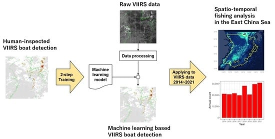
2.1. Overview of the Machine Learning Model

The present VBD algorithm uses a machine learning model as a key component. Figure 1 demonstrates the flowchart of the machine learning-based VBD algorithm, and Figure 2 shows the schematic process of model development. For generating VBD output, our algorithm uses two kinds of VIIRS data, i.e., VIIRS day–night band (DNB) and the cloud mask (CM), as input. After processing the raw VIIRS data, a machine learning model (i.e., the production model in Figure 1) is applied to each pixel of the processed VIIRS data. This determines whether each pixel corresponds to a vessel or a non-vessel pixel. For training the machine learning model, we used the existing VBD output of FRA [14] as an objective of the training. The details of the data and its processing are described below.

2.2. Data

2.2.1. Raw VIIRS Data

Historical VIIRS data of the Suomi NPP satellite were obtained from the Comprehensive Large Array-Data Stewardship System (CLASS) of NOAA (https://www.avl.class.noaa.gov/, accessed on 20 May 2022). Specifically, the VIIRS day–night band SDR (DNB) data and the VIIRS cloud mask EDR (CM) data from 1 January 2014 to 10 May 2022 were used as source data for our algorithm.

2.2.2. VIIRS Boat Detection Data

Two different VBD data were used in this study. One VBD dataset was developed by FRA [14], covering major light luring fishing around Japan, which was also the primary monitoring target of present study (Figure 3). We used this dataset as training data for our algorithm. Another VBD dataset was developed by EOG [13], and we used it to compare detection outputs.

2.2.3. On-Ship Radar Data

To evaluate the performance of our VBD algorithm, we used independent vessel detection data collected by an FRA research vessel, Yoko-maru. The research vessel collected the positions of the other vessels around it using its on-ship radar device. The on-ship radar data were acquired with a time difference of less than 8 min compared to the VIIRS observations. A total of 41 days of radar data from 22 February 2017 to 20 October 2019 were used to evaluate our algorithm.

2.3. Development of the Machine Learning Model

2.3.1. Preprocessing

Following Elvidge et al. (2015) [13], we applied three steps of preprocessing to DNB data including (1) converting the DNB radiance unit from watts/cm²/sr to nanowatts/cm²/sr for readability, (2) taking the logarithm of the radiance to enhance the contrast, and (3) applying the adaptive Wiener filter to reduce the noise observed at the edges of the scan [29].

2.3.2. Creating Features for Detection

Our algorithm determines whether each DNB pixel is a vessel or not on the basis of the following features. The following features are used as explanatory variables when training the machine learning model.

• Log₁₀ (DNB radiance)
• Spike median index (using 3 × 3, 5 × 5, 7 × 7, 9 × 9 surrounding pixels)
• Spike height index (using 3 × 3 surrounding pixels)
• Maximum integer cloud mask (using 3 × 3, 5 × 5, 7 × 7, 9 × 9 surrounding pixels)
• Moon illumination
• Zenith angle of the satellite
• Zenith angle of the moon
• Zenith angle of the sun

Spike Median Index

We adopt the spike median index ($SMI$) and spike height index (SHI) proposed by Elvidge et al. (2015) while using broader surrounding pixels for $SMI$ (from 3 × 3 to 9 × 9 pixels) as defined in the following equation to take a blurred spike of vessel light into account:

$$SM{I}_{s\times s}=lo{g}_{10}\left(R_{center}\right)-lo{g}_{10}\left(Median\left(R_{s\times s}\right)\right),$$

where $SM{I}_{s\times s}$ indicates the $SMI$ value calculated from the surrounding pixels of size $s$, $R_{center}$ indicates the radiance value of the subject DNB pixel, and $R_{s\times s}$ indicates the set of radiance values of DNB pixels of the surrounding range of $s$ (Figure S1).

The value of SMI indicates how much brighter the target pixel is than the surrounding pixels. The threshold of SMI values for 3 × 3 surrounding pixels is a key part of the EOG algorithm, but this threshold is effective only for clear sky conditions. The appearance of a vessel’s light and moonlight reflection from the clouds varies greatly depending on the moon/cloud conditions. Thus, a single threshold from a single variable is insufficient to distinguish a vessel’s light from varying background light. Using SMI values of various ranges of surrounding pixels as explanatory variables can address this limitation.

Maximum Integer Cloud Mask

The integer cloud mask value of CM data is used to incorporate cloudiness information into our algorithm (0: confident clear, 1: probably clear, 2: probably cloudy, 3: confident cloudy). As the CM data have a higher spatial resolution (375 m) than DNB images (750 m), the information from the nearest cloud mask pixel is assigned to each DNB pixel. Then, a maximum cloud mask value from the surrounding DNB pixels (in window sizes ranging from 3 × 3 to 9 × 9 pixels) is calculated. As the range of surrounding pixels becomes broader, the subject pixel is more likely to be judged as cloudy. The maximum cloud mask value indicates the presence of clouds around the subject pixels and is used to train the machine learning model to reduce false detection due to clouds.

Moon Illumination

Moon glint is one of the major possible causes of false detections and needs to be taken into account. The value of moon illumination is retrieved from the geolocation file of the DNB data. It ranges from 0 to 100, where 0 indicates a new moon, and 100 represents a full moon.

Zenith Angles of Satellite, Moon, and Sun

The zenith angles of the satellite can influence the level of light reflection from the moon and the sun. As the satellite’s zenith angle becomes greater (i.e., the edge region of the scan), the noise level of the DNB image increases [13]. For this study, the satellite’s zenith angles are retrieved from the DNB geolocation file.

Objective Variable

Our algorithm is developed on the basis of FRA’s VBD. We set DNB pixels corresponding to FRA’s VBD as positive pixels (vessel pixels) while the other pixels are marked as negative pixels (non-vessel pixels).

Extracting Local Maximum Pixels

With the features described above, only DNB pixels that have a local maximum radiance in the 3 × 3 surrounding area are extracted to reduce the number of pixels to be used in the machine learning model. The local maximum serves as the minimum requirement for the subject pixel to be determined as a vessel. Likewise, the FRA and EOG algorithms require that a pixel be a local maximum when determining vessel detection.

2.3.3. Modeling Design

After processing raw VIIRS data, the below-described procedures are applied before feeding the data into the machine learning algorithm.

Splitting Train/Test Set

A total of 905 days (from 5 January 2017 to 10 March 2020) of data were available for modeling. These are the dates on which we retained both FRA’s VBD data and the VIIRS raw data. We split the entire data into training and testing data according to the day (Figure S2A), randomly extracting 40 days per month over 3 years for training (total 480 days) and 15 days per month over 3 years for testing (total 180 days) (Figure S2B). We extracted the same number of days from each month to ensure that the training/testing data were seasonally unbiased. This unbiased sampling is required for testing the model’s performance because fishing activities and cloud conditions are affected by season.

The Machine Learning Algorithm

We adopted random forest for our machine learning model, using the ranger package [30] in R 4.0.3. We adopted the two-step approach described in Figure 2 for model training. We used fewer training data to train the first model (baseline model). After examining its detection output, we then used more training data to train the second model (production model) supplementing the baseline model to generate the final detection result.

To create training data for both the baseline and production models, we used the same 480 days for training. It consisted of roughly 1.5 million pixels per day and a maximum of 7000 vessel detections per day. As the number of pixels was high and the ratio of positive pixels to negative pixels as highly imbalanced, efficient sampling was essential.

Creating the Training Data for the Baseline Model

For the baseline model, we created training data by collecting all positive pixels (i.e., vessel pixels) and 20,000 negative pixels (i.e., non-vessel pixels) per day from the training dates. For the sampling of negative pixels, we took the following steps for each day to keep the radiance variation of the negative pixels in the training data:

• Extract negative pixels whose log₁₀ (radiance) is greater than [min{log₁₀ (radiance of positive pixels)} − 1].
• Divide the range of radiance of the extracted negative pixels into 10 classes evenly on the log scale.
• Randomly sample negative pixels without replacement evenly from these 10 radiance classes until the total number of sampled negative pixels reaches 20,000 pixels.

Creating the Training Data for the Production Model

We applied the trained baseline model to all the pixels in the training dates and obtained false-positive and false-negative pixels. Next, we added these pixels to the original training data of the baseline model to create the training data for the production model. This step allows the production model to reduce false positives compared to the baseline model. By including the false-positive pixels in the training data of the production model, the model could be trained to better classify these undesired pixels as negative pixels.

Hyperparameter Setting

We used the same hyperparameter settings when training random forest to create both baseline and production models (

Table 1. The hyperparameter settings of random forest used to train the baseline and production models.

Hyperparameter	Value	Explanation
N_tree	50	The number of trees in the ensemble
N_val	3	The number of variables randomly sampled at each split when creating the tree models
Min_n	316	The minimum number of data points in a node required for the node to be split further

). The same hyperparameter value was independently determined as the optimal value for the baseline and production training data.

The first and second hyperparameters in Table 1 were set empirically to restrict the size of the model (several values were tried but did not affect the results significantly), while the third hyperparameter was determined by fivefold cross-validation on the training data of the baseline/production model to control the model complexity. We used the area under the precision–recall curve (PR_AUC) to determine these hyperparameter values.

2.4. Evaluation of VBD with On-Ship Radar Data

We used vessel position data collected through on-ship radar aboard a Japanese research vessel (observer vessel) to evaluate the VBD’s performance. For this evaluation, we followed the steps described below.

2.4.1. Extracting VIIRS Detections within Radar Range

On-ship radar devices sometimes do not detect vessels that are far away from the radar even within its theoretical detection range. We, thus, considered the detection limit of the on-ship radar as the distance to the farthest vessel detection from the radar. Only VBD data within this distance from the observer vessel were included in the evaluation process.

2.4.2. Distance Threshold for Matching VBD and On-Ship Radar Data

The on-ship radar data were recorded at a time close to the VBD acquisition times (with a time gap between 1 and 8 min). As the maximum distance that a vessel can travel during this time gap is negligible, we simply considered the closest pairs of VIIRS detection and on-ship radar detection with a distance of less than 2000 m a match. To determine this distance threshold, we first unified three VBDs (i.e., present study, FRA, and EOG) into a single VBD by merging overlapping detections. Then, we plotted unified VBD and on-ship radar detections simultaneously for each night and visually examined the results to confirm that the threshold accurately determined the matching between VBD and on-ship radar detections.

2.4.3. Selection of On-Ship Radar Data Used for Evaluation

As on-ship radar devices can fail to detect some vessels present around the radar, we selected only nights when the on-ship radar detected all the obvious lit vessels present around the observer vessels by visually examining the unified VBD and DNB images together to ensure the consistency of the data used in the evaluation process. This step allowed us to choose scenes conservatively so that VIIRS detections unmatched to on-ship radar detections in these scenes were considered to be actual false detections of VBDs. Notably, this procedure was executed with unified (and anonymized) VBD data to avoid biases when comparing the detection performance between three VBD algorithms.

2.4.4. Metrics to Evaluate the Detection Performance of VBD Algorithms

We evaluated the performance of the three VBD algorithms for each night using the following metrics: $Precision$, $Recall$, and $F1 score$. Then, a nonparametric pairwise comparison test was conducted to evaluate the statistical significance of the difference in the performance metrics between the new algorithm and the existing algorithms. The metrics for each night and VBD algorithm were calculated as follows:

$$Precision=\frac{N_{vm}}{N_v},$$

(1)

$$Recall=\frac{N_{vm}}{N_r},$$

(2)

$$F1 score=\frac{2\times Precision\times Recall}{Precision+Recall},$$

(3)

where $N_{vm}$ is the number of VIIRS detections matched to on-ship radar detections for a night for a VBD algorithm, $N_v$ is the number of VIIRS detections of a VBD algorithm in the radar range for a night, and $N_r$ is the number of on-ship radar detections for a night.

2.5. VBD Data Analysis in the East China Sea

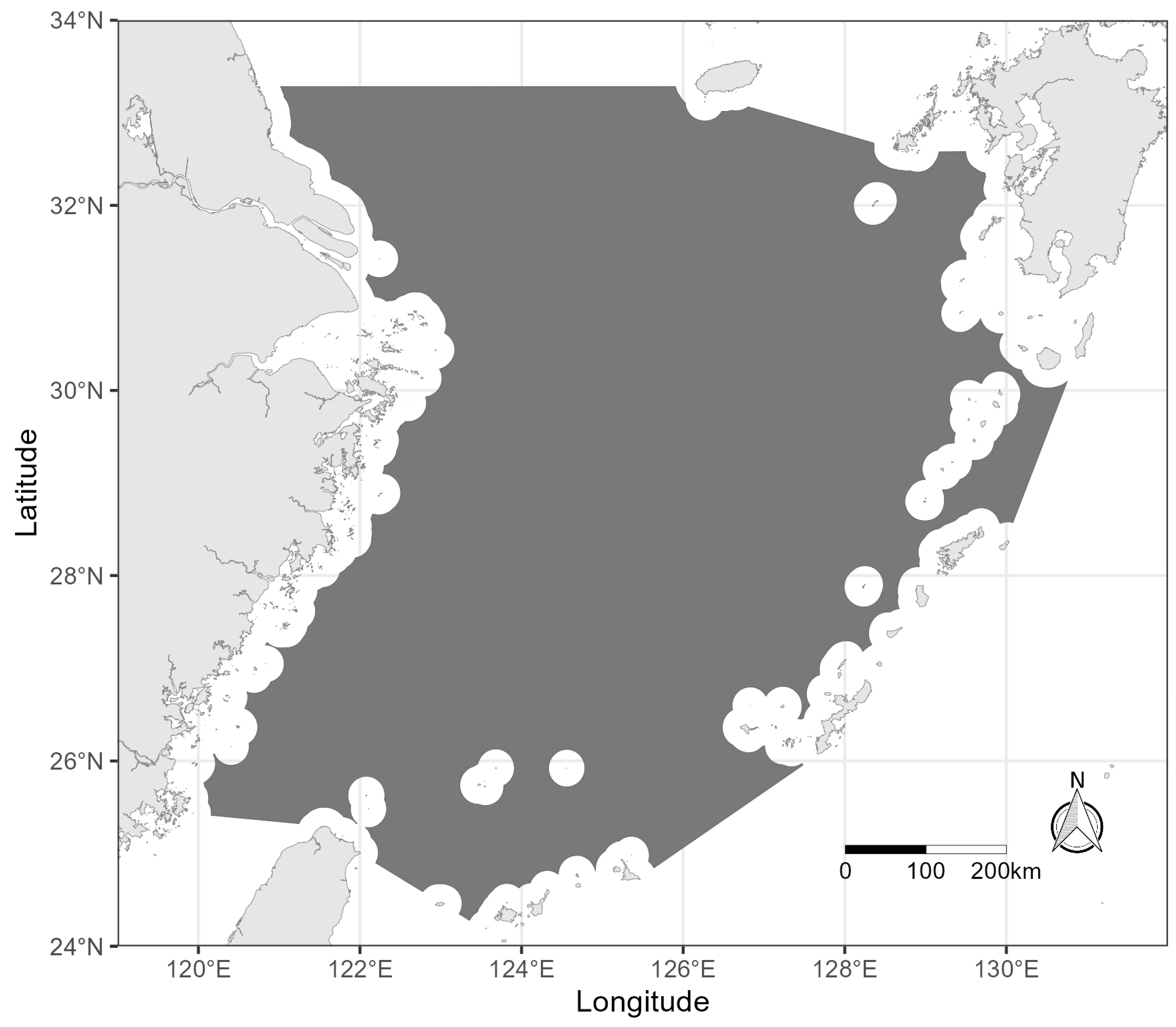
2.5.1. Study Area

By applying our machine learning-based VBD algorithm to past VIIRS data, we can analyzed long-term historical activities of light-fishing vessels in the East China Sea in an automated and consistent manner. For this analysis, we set the study area shown in Figure 4 and compared the VBDs generated by our algorithm and other VBD algorithms. We excluded areas within 12 nautical miles from the shore in our study, as the VBD algorithms are likely to perform poorly in areas of high vessel densities due to the low resolution of the DNB images, particularly near the coasts, and produce more false detections due to lights from land.

2.5.2. Eliminating Overlapping Observations from VBD

As the Suomi NPP satellite can observe the same area multiple times per night, we eliminated the overlapping observations to better capture fishing activities from the VBD data. As each satellite’s overpass can be distinguished by orbit number, we selected the orbit number with the smallest satellite zenith angle for each gridded area (0.1°) for each day.

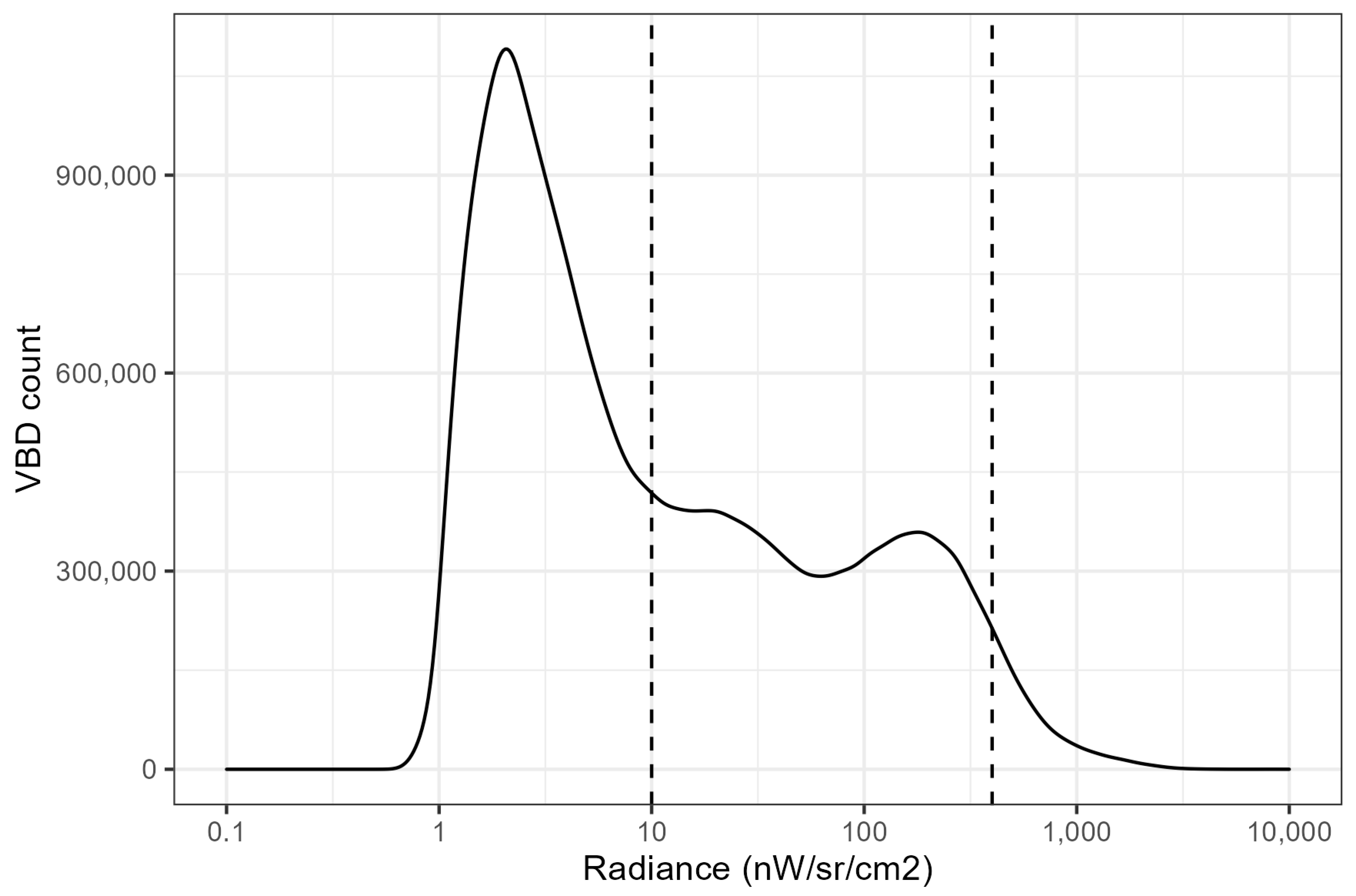
2.5.3. Inferring the Fishing Activities from VBD

When the moon is shining brightly, the brightness of the background ocean is increased from the perspective of the VIIRS sensor by the reflection of the moonlight from the sea surface, making it difficult to distinguish between the background ocean and the lights of vessels. This effect, in general, decreases the number of detections when the date comes closer to a full-moon night and increases the number of detections when the date comes closer to a new-moon night (Figure S4). To estimate the fishing activities from the VBD data more accurately than simple daily counting, we chose the dates when we observed the largest daily count of VIIRS detections in every half-month period as proposed by Park et al. (2020) [6]. This allowed us to minimize the influence of the cloud and moon. For the total annual vessel days, we assumed that the number of vessels operating in a given region would be the same as the maximum daily count for a given half-month period.

3. Results

3.1. Model Evaluation

3.1.1. Detection Performance against Training and Testing Data

We applied the production model to all pixels in the DNB images from the training and testing data to evaluate the model’s performance. The performance was evaluated using the precision–recall curve (PR curve) against FRA’s VBD and its area under curve value (PR-AUC) (Figure 5). According to the shape of the PR curve, we considered the score 0.4 as the threshold value for vessel detection (i.e., the pixels having a score greater than 0.4 were considered as vessel detection). The values of precision and recall against FRA’s detections at the score threshold of 0.4 were 0.67 and 0.83, respectively, in the testing data, which means that 83% of the vessels detected by FRA’s algorithm were also detected by the production model, and 67% of the vessels detected by the production model were also detected by FRA’s algorithm. Additionally, we visually examined the detections in all testing data along with the DNB images to ensure that the production model with the score threshold of 0.4 produced very few obvious false positives.

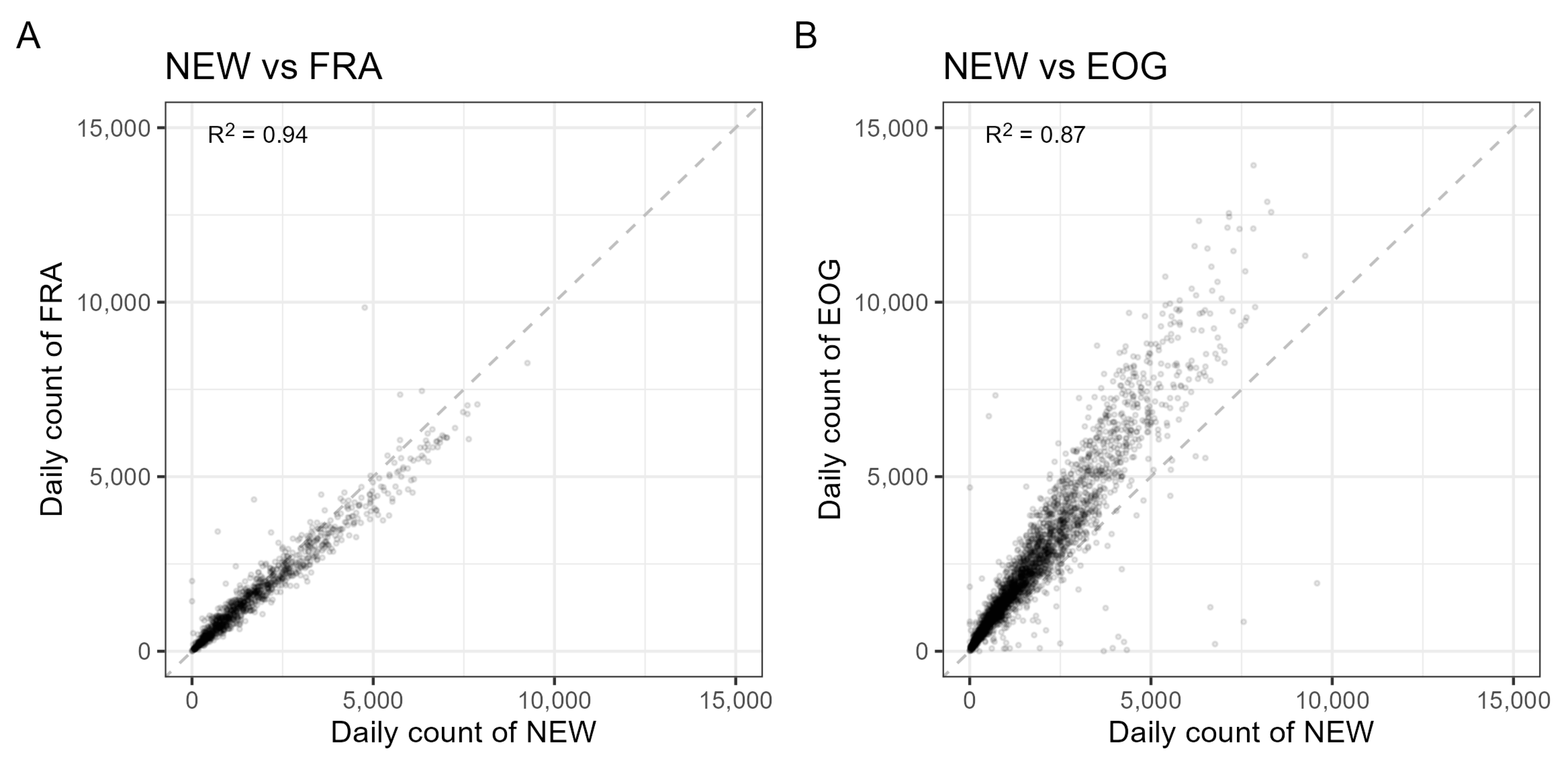
3.1.2. Comparison of the Model VBD with Existing VBDs

The daily counts of vessel detections were compared to examine the difference between the model VBD of this study and the existing VBDs including FRA and EOG (Figure 6). The overlapping VIIRS observations on the same night were removed before calculating the daily count of VBDs. The daily count of our algorithm was largely consistent with both FRA and EOG, but it generally detected slightly more than the FRA algorithm abut lower than the EOG algorithm (Figure 6).

Figure 7 shows the radiance distribution of these three VBDs. The most remarkable difference in radiance distribution among the three VBD algorithms is that the EOG algorithm produced far more detections with a lower radiance than our algorithm and the FRA algorithm, which led to very few detections with a radiance lower than 1 nW/sr/cm². The differences among the three algorithms generally became smaller when the radiance became greater.

When focusing on the difference in the total number of detections, or the height of the graphs in Figure 7, the differences were consistent with the difference in the number of daily counts among the three VBDs in Figure 6; thus, the larger daily count in EOG could be explained by the larger number of detections with a lower radiance.

3.1.3. Evaluation with On-Ship Radar Data

Figure 8 shows an example of the on-ship radar image we used for the evaluation of VBD algorithms.

To analyze the differences in the detection performance of the VBD algorithms, the precision, recall, and F1 score are calculated for each night and VBD algorithm. Low precision indicates a high rate of false detections (i.e., noise), and low recall indicates that a VBD algorithm detects only a few radar detections (i.e., low sensitivity). The F1 score is defined as a harmonic mean of precision and recall to represent the overall performance of the models. The paired Wilcoxon rank sum test showed no statistically significant differences among the three VBD algorithms (Figure 9). Despite no statistically significant differences in the results, the proposed model and FRA VBDs were more sensitive to detection when clouds were present, whereas the EOG algorithm was more sensitive when there were no clouds and moon (Figure S5).

3.2. Analysis of the East China Sea

To analyze the long-term change of light fishing vessel activities in the study area, we first partitioned VIIRS detection into three radiance classes (Figure 10). The three classes (<10, 10–400, and 400 < nW/sr/cm²) largely correspond to radiance ranges of fishing gear types and flag states revealed in the previous study [27]. Although the first class (<10 nW/sr/cm²) was not reported in the previous study, it likely corresponds to non-light-luring fishing vessels prominent in this region such as trawlers and non-fishing vessels. Vessels with a radiance between 10 and 60 nW/sr/cm² are believed to correspond to the Chinese Taipei light lift net and Japanese light vessels with reduced operational light levels. The radiance class of 60–400 nW/sr/cm² corresponds to major light-luring fishing vessels with normal operational light levels, notably the Chinese lit falling net, Chinese lit lift net, Chinese “tra-ami”, Chinese Taipei lit lift net, and Japanese light fishing vessels. The radiance levels of 10–60 and 60–400 correspond to typical light-luring fishing and showed the same spatiotemporal pattern; we treated these levels as a single, combined radiance class in the analysis. We separated detections with radiances greater than 400 nW/sr/cm² as Chinese lit-falling net vessels, which are reported to have far greater radiance than other types of light-luring vessels.

Examining the spatial distribution of the detections (Figure 11), the detections with radiance < 10 nW/sr/cm² were more evenly spread spatially within the continental shelf of the East China Sea compared to the detections with greater radiances. Focusing on the radiance classes presumably representing light-luring fishing (10~400 and >400 nW/sr/cm²), these detections were concentrated around the northeastern part of the study area (around 32°N, 127°E) and the southern part of the analysis area (around 27°N, 124°E). In particular, the detections with radiance greater than 400 nW/sr/cm² were more often observed in the northeastern part of the study area.

To analyze the temporal changes in fishing activities over the years, the daily count and the yearly aggregate of the detections in the study area were calculated from 2014 to 2021 (Figure 12). The result shows that the VBD with radiance lower than 10 nW/sr/cm² decreased over the analysis period, whereas the detections with radiance between 10 and 400 nW/sr/cm² were generally unchanged except for a temporal drop in the middle of the period. On the contrary, the VBD with radiance greater than 400 increased since 2018, especially in the northeast part of the study area (Figure S6).

To evaluate the seasonal changes in the number of operating fishing vessels in the area, the maximum daily count of detections for each year and month was determined (Figure 13). For radiance < 10 nW/sr/cm², a smaller number of detections were more often observed since 2017, especially in months when a relatively large number of detections were observed before 2017 (i.e., January, May, September, and October), while a slight increase in 2021 was observed in the winter season (i.e., January, February, and December), consistent with the result in the annual aggregation of the detection count (Figure 12). For radiance 10–400 nW/sr/cm², a large decrease in VBD count was observed in July since 2017. On the other hand, for radiance greater than 400 nW/sr/cm², the VBD count increased recently from August to December, consistent with the annual aggregated detection count (Figure 12).

While the goal of our study was to automate the FRA VBD, we also conducted the same ECS analysis using the EOG VBD (Figures S7 and S8); qualitatively similar results were obtained. However, as expected, EOG generally had more detections, especially in the low-radiance class, while the medium- and high-radiance classes did not differ significantly.

4. Discussion

4.1. Model Evaluation

Our machine learning-based VBD algorithm reproduced FRA’s human-inspected algorithm output in an automatic and consistent manner. The present new algorithm generated similar detection results to the FRA algorithm (83% of FRA detections were detected by our algorithm, and 67% of our detections were detected by FRA). With some exceptions, our model generally detected more vessels compared to the FRA model (Figure 6). In the FRA algorithm, the daily radiance thresholds were determined by analysts to distinguish vessel detections from the background noise under several conditions based on the presence of clouds and the moon [14]. Those thresholds are determined with a focus on suppressing noise, and true vessels are often excluded. On the contrary, our VBD algorithm keeps these vessels because it determines vessels on the basis of various features of local surrounding pixels. In addition, we visually inspected these vessels and confirmed that they were unlikely to be false positives.

Compared to the EOG algorithm, our algorithm tended to detect vessels more conservatively. A notable difference between the two algorithms is that the EOG algorithm produced more detections with low radiance. One possible reason is that the EOG algorithm relies mainly on the ratio of radiance between the target pixel and a small window (3 × 3) of surrounding pixels (i.e., SMI_3×3), which leads the EOG algorithm to detect a target pixel as a vessel even when the pixel is too dim for a human analyst to determine it as such [13]. In comparison, our model uses both the absolute radiance value of a target pixel (inherited from the FRA algorithm) and a broader window of surrounding pixels in the DNB image (maximum 9 × 9 pixels) as important features. This difference allows our algorithm to identify pixels that are more discernible by the human eye.

We evaluated the performance of the three different VBD algorithms using independent vessel detection data collected by a research vessel (Figure 8). This evaluation showed that our algorithm performed consistently with the existing FRA human-inspected VBD, showing no statistically significant difference. Given that the primary goal of our algorithm was to produce long-term and region-specific detections in an automatic and consistent manner on the basis of the FRA VBD, it is reasonable that our algorithm performance was not statistically different from the FRA algorithm. Although the evaluation also demonstrated no statistically significant differences with the EOG algorithm, it is possible that our model performance could be different from the EOG algorithm considering the differences in the radiance distribution shown in Figure 7. The observed similar performance was likely due to the small sample size of the radar data available for evaluation and the possible absence of vessels with a small radiance in the sample data. In addition, as on-ship radar sometimes fails to detect some vessels within its range of observation, a further step in selecting scenes with no obvious non-detection of all lit vessels was required in this study. This step might have caused an upward bias in the precision value (i.e., underestimating the false-positive rate). While our evaluation with on-ship radar data was sufficient to demonstrate that our algorithm is comparable to existing algorithms, obtaining more on-ship radar data in various locations and conditions is necessary to perform a more comprehensive evaluation of the absolute performance of VBD algorithms.

4.2. East China Sea Analysis

In this study, we classified vessel detection into three classes (Figure 10), according to a previous study that identified fishing vessel classes in the East China Sea with their corresponding brightness [27]. Overall spatial and seasonal patterns of the detection generally correspond to common fishing and weather conditions in this region. For example, the low-radiance class (<10 nW/sr/cm²) corresponds to the reported fishing ground of trawlers [31], and medium- to high-radiance classes (10–400 nW/sr/cm² and >400 nW/sr/cm²) correspond to light luring fishing [32]. This region experiences occasional typhoons from July to September, which might be one of the reasons for the annual fluctuation in VBD counts across years from July to September, whereas windy rough weather in November to January may also explain the decrease in VBD counts in the winter season (Figure 13).

On the other hand, some temporal changes across years in the VBD count appear to correspond to recent policy changes. The summer fishing moratorium by the Chinese government started in 1998 covering the Bohai Sea, the Yellow Sea, the East China Sea, and the northern part of the South China Sea, running from May to September, while the exact periods and the areas differ depending on the years and types of fishing [33,34]. The monthly fishing activities sharply declined after 2017 for the low-radiance class in May and for the high-radiance class in July (Figure 13). This decline could be possibly explained by an extension of the moratorium period from 2017, although the exact details of the moratorium are unknown. While the activities of the medium-radiance class also decreased since 2017 in July, it rather increased in later years, particularly in April and from August to December (Figure 13). Given that annual fishing activity did not change significantly throughout the observation period (Figure 12), this change suggests that the medium-radiance class vessels might have shifted their fishing activity to the non-moratorium season.

Looking at the annual trend over the study period (Figure 13), fishing activities by vessels of the low-radiance class decreased significantly in 2017 and remained low since, whereas fishing activities by vessels of the medium-radiance class stayed at the same level except for a temporal drop in the middle of the study period. On the contrary, as for the vessels of the highest radiance class, which appeared to drastically increase in the last two years, it is possible that this increase may have been caused by an overall increase in the total number of bright vessels in the region or by a shift of fishing operations from other regions, given the reported sharp decrease in the number of vessels of the same brightness in North Korean water [6,35]; however, further research is needed to determine the origin of these vessels. A previous study based on AIS information claimed that overall fishing efforts have remained unchanged, but have shifted from the period of summer moratorium to the regular fishing season for coastal fisheries [36]. Our study showed that this trend is also applicable to offshore light-luring fishing, which cannot be monitored by AIS, with the exception of an increase in particularly bright vessels in recent years.

The application of the machine learning-based algorithm to the East China Sea enables us to analyze temporal trends of fishing in the region where other satellite monitoring techniques including AIS remain limited [37]. Additionally, using the machine learning-based VIIRS boat detection model more consistently and automatically offers public information on the fishing activity in the region. The information is, however, limited to the presence of light-luring vessels used as a proxy for their daily activity. For a better estimation of resource extraction and the management of the fisheries in the East China Sea, it is necessary to link fishing activities estimated from VIIRS data to catch information from relevant countries in the region.

4.3. Technical Implications

We developed a machine learning-based VIIRS boat detection algorithm based on an existing algorithm which requires manual inspection by analysts. Since it is generally difficult to guarantee the reliability of VIIRS detection through independent vessel detection technologies such as AIS and SAR due to limited effectiveness in East Asia, it is worthwhile to guarantee fishing activities by VIIRS through human inspection. However, relying on the experience of experts and manual work is unsustainable for continuous and extensive monitoring. It is, therefore, reasonable to build a machine learning-based algorithm to reproduce the existing VBD.

Applying machine learning to VIIRS night light data for vessel detection was challenging due to the large data size and imbalanced nature of vessel vs. non-vessel pixels, i.e., 1:3000 after extracting local maximum pixels. Since the absolute number of non-vessel pixels is large, a simple random sampling of non-vessel pixels is ineffective to learn the entire characteristics of non-vessel pixels. A model created by such a simple approach is prone to generate a large number of false positives when applied to testing data. The imbalanced nature of VIIRS night light data in vessel detection requires a particular approach. An oversampling approach of a minor class such as SMOTE is popular when dealing with imbalanced data [38]; however, the approach was inapplicable in our case due to the large size of the major class (i.e., non-vessel pixels). Bagging of multiple models is an alternative option where multiple model outputs averaged from different sampling of the major class while sampling the entire minor class is used as final output [39]. However, the bagging of 10 models was insufficient to resolve the false positives in our case due to a large number of negative pixels. Since our model is intended to be used in actual monitoring operations, we wanted to avoid a bagging model that requires many sub-models. Ultimately, an efficient down-sampling design of the major class was key to building an appropriate machine learning model in our case. Our two-step approach for the efficient down-sampling of the major class proved to be effective for training on big and imbalanced datasets, offering other machine learning practitioners a useful application case.

Our methodology paves the way for evaluating the temporal variation of fishing activity by light-luring vessels; however, several caveats exist. First, light from vessels may not be detected by VIIRS because it is obscured by clouds or the moon. We minimized this limitation by using a window of 15 days when estimating the fishing activities in the region, following Park et al. (2020). This assumption reasonably captures the real number of lit vessels operating in these areas over that period because most of these offshore vessels fish in a given location for longer than 2 weeks. Second, VIIRS has a resolution of 750 m, which does not allow distinguishing multiple vessels in a single pixel. Vessels of mid- or high-radiance level are unlikely to operate within such a short distance. However, low-radiance trawlers in this region often operate in pairs, so-called pair trawlers [40], and the VIIRS cannot distinguish these pair vessels. Third, the number of detections with low radiance (<10 nW/cm²/sr) in our algorithm was much smaller compared to EOG; thus, it is possible that our algorithm may have missed vessels of this class. Given these considerations, it is important to recognize that quantitative analysis using our VIIRS detection tends to underestimate (especially for vessels with small radiance), whereas this effect is not significant for the vessels of a medium- and high-radiance level.

The methodological approach presented in this study might be useful for fishing monitoring in other regions where light-luring fishing is intense and comes with other technical challenges. For instance, in South America, monitoring of light fishing vessels by existing VBD is disrupted by a significant number of false detections because of the abundance of high-energy particles in the region, which affects the electronic systems on the satellite, known as the South America Anomaly [41]. The conditions for removing these noises are unknown; however, by visually labeling only true vessel detection to train a machine learning model, one may be able to obtain detection results without the noise.

The lack of data indicating the presence of true vessels and the high variability in the appearance of VIIRS images due to clouds and the moon are major challenges in vessel detection using VIIRS data. In this study, a two-step machine learning based on existing VBD outputs visually inspected by humans and artificial features (i.e., SMI) was used to tackle these issues. In other major satellite data, such as SAR, approaches using transition learning of deep learning models have been attempted for similar issues [42,43,44]. It may also be worthwhile to try approaches that use deep learning with limited true vessel presence data and no artificial features for VIIRS.

5. Conclusions

The algorithm and the machine learning approach applied in this study represent a step forward in monitoring the long-term temporal activity of light-luring fishing. This new approach also allows automatic detection, ensuring scalability and consistency when applied to large areas, as well as sheds light on fishing activities in areas where holistic fishery management is challenging for both political and technical reasons. For instance, a lack of shared fishery information hinders relevant nations from collaborating on regional fishery resource assessments [28]. From the technical perspective, other satellite monitoring data such as SAR and AIS are scarce in the region for examining fishing activities due to the coverage issues [37]. Although each country has its own vessel monitoring systems or VMS, they are of private nature and contribute less to the transparent management of shared fisheries. This study on machine learning-based VBD is expected to fill in this gap, albeit partially, with respect to public information for fishery management. The two-step approach we adopted for training the machine learning model might also have general applicability for other large imbalanced data. This would provide a promising option for practitioners considering machine learning applications for satellite data.

References

1. Kataoka, C. The new fisheries regime and fisheries adjustment among Japan, China and Korea. Nippon Suisan Gakkaishi 2011, 77, 699–701. (In Japanese) [Google Scholar] [CrossRef] [Green Version]
2. McCauley, D.J.; Woods, P.; Sullivan, B.; Bergman, B.; Jablonicky, C.; Roan, A.; Hirshfield, M.; Boerder, K.; Worm, B. Ending Hide and Seek at Sea. Science 2016, 351, 1148–1150. [Google Scholar] [CrossRef] [PubMed] [Green Version]
3. Kroodsma, D.A.; Mayorga, J.; Hochberg, T.; Miller, N.A.; Boerder, K.; Ferretti, F.; Wilson, A.; Bergman, B.; White, T.D.; Block, B.A.; et al. Tracking the Global Footprint of Fisheries. Science 2018, 359, 904–908. [Google Scholar] [CrossRef] [PubMed] [Green Version]
4. Kroodsma, D.A.; Hochberg, T.; Davis, P.B.; Paolo, F.S.; Joo, R.; Wong, B.A. Revealing the Global Longline Fleet with Satellite Radar. Sci. Rep. 2022, 12, 21004. [Google Scholar] [CrossRef] [PubMed]
5. Miller, N.A.; Roan, A.; Hochberg, T.; Amos, J.; Kroodsma, D.A. Identifying Global Patterns of Transshipment Behavior. Front. Mar. Sci. 2018, 5, 240. [Google Scholar] [CrossRef] [Green Version]
6. Park, J.; Lee, J.; Seto, K.; Hochberg, T.; Wong, B.A.; Miller, N.A.; Takasaki, K.; Kubota, H.; Oozeki, Y.; Doshi, S.; et al. Illuminating Dark Fishing Fleets in North Korea. Sci. Adv. 2020, 6, eabb1197. [Google Scholar] [CrossRef]
7. Welch, H.; Clavelle, T.; White, T.D.; Cimino, M.A.; Van Osdel, J.; Hochberg, T.; Kroodsma, D.; Hazen, E.L. Hot Spots of Unseen Fishing Vessels. Sci. Adv. 2022, 8, eabq2109. [Google Scholar] [CrossRef]
8. Kanjir, U.; Greidanus, H.; Oštir, K. Vessel Detection and Classification from Spaceborne Optical Images: A Literature Survey. Remote Sens. Environ. 2018, 207, 1–26. [Google Scholar] [CrossRef]
9. Straka, W.C.; Seaman, C.J.; Baugh, K.; Cole, K.; Stevens, E.; Miller, S.D. Utilization of the Suomi National Polar-Orbiting Partnership (NPP) Visible Infrared Imaging Radiometer Suite (VIIRS) Day/Night Band for Arctic Ship Tracking and Fisheries Management. Remote Sens. 2015, 7, 971–989. [Google Scholar] [CrossRef] [Green Version]
10. Miller, S.D.; Mills, S.P.; Elvidge, C.D.; Lindsey, D.T.; Lee, T.F.; Hawkins, J.D. Suomi Satellite Brings to Light a Unique Frontier of Nighttime Environmental Sensing Capabilities. Proc. Natl. Acad. Sci. USA 2012, 109, 15706–15711. [Google Scholar] [CrossRef] [Green Version]
11. Miller, S.D.; Straka, W.; Mills, S.P.; Elvidge, C.D.; Lee, T.F.; Solbrig, J.; Walther, A.; Heidinger, A.K.; Weiss, S.C. Illuminating the Capabilities of the Suomi National Polar-Orbiting Partnership (NPP) Visible Infrared Imaging Radiometer Suite (VIIRS) Day/Night Band. Remote Sens. 2013, 5, 6717–6766. [Google Scholar] [CrossRef] [Green Version]
12. Levin, N.; Kyba, C.C.M.; Zhang, Q.; Sánchez de Miguel, A.; Román, M.O.; Li, X.; Portnov, B.A.; Molthan, A.L.; Jechow, A.; Miller, S.D.; et al. Remote Sensing of Night Lights: A Review and an Outlook for the Future. Remote Sens. Environ. 2020, 237, 111443. [Google Scholar] [CrossRef]
13. Elvidge, C.D.; Zhizhin, M.; Baugh, K.; Hsu, F.-C. Automatic Boat Identification System for VIIRS Low Light Imaging Data. Remote Sens. 2015, 7, 3020–3036. [Google Scholar] [CrossRef] [Green Version]
14. Oozeki, Y.; Inagake, D.; Saito, T.; Okazaki, M.; Fusejima, I.; Hotai, M.; Watanabe, T.; Sugisaki, H.; Miyahara, M. Reliable Estimation of IUU Fishing Catch Amounts in the Northwestern Pacific Adjacent to the Japanese EEZ: Potential for Usage of Satellite Remote Sensing Images. Mar. Policy 2018, 88, 64–74. [Google Scholar] [CrossRef]
15. Elvidge, C.D.; Ghosh, T.; Baugh, K.; Zhizhin, M.; Hsu, F.-C.; Katada, N.S.; Penalosa, W.; Hung, B.Q. Rating the Effectiveness of Fishery Closures With Visible Infrared Imaging Radiometer Suite Boat Detection Data. Front. Mar. Sci. 2018, 5, 132. [Google Scholar] [CrossRef]
16. Geronimo, R.C.; Franklin, E.C.; Brainard, R.E.; Elvidge, C.D.; Santos, M.D.; Venegas, R.; Mora, C. Mapping Fishing Activities and Suitable Fishing Grounds Using Nighttime Satellite Images and Maximum Entropy Modelling. Remote Sens. 2018, 10, 1604. [Google Scholar] [CrossRef] [Green Version]
17. Hsu, F.-C.; Elvidge, C.D.; Baugh, K.; Zhizhin, M.; Ghosh, T.; Kroodsma, D.; Susanto, A.; Budy, W.; Riyanto, M.; Nurzeha, R.; et al. Cross-Matching VIIRS Boat Detections with Vessel Monitoring System Tracks in Indonesia. Remote Sens. 2019, 11, 995. [Google Scholar] [CrossRef] [Green Version]
18. Cozzolino, E.; Lasta, C.A. Use of VIIRS DNB Satellite Images to Detect Jigger Ships Involved in the Illex argentinus Fishery. Remote Sens. Appl. Soc. Environ. 2016, 4, 167–178. [Google Scholar] [CrossRef]
19. Lebona, B.; Kleynhans, W.; Celik, T.; Mdakane, L. Ship Detection Using VIIRS Sensor Specific Data. In Proceedings of the 2016 IEEE International Geoscience and Remote Sensing Symposium (IGARSS), Beijing, China, 10–15 July 2016; pp. 1245–1247. [Google Scholar]
20. Xue, G. Bilateral Fisheries Agreements for the Cooperative Management of the Shared Resources of the China Seas: A Note. Ocean Dev. Int. Law 2005, 36, 363–374. [Google Scholar] [CrossRef]
21. Tokimura, M. Fisheries and Their Resources in the East China Sea. Nippon Suisan Gakkaishi 2011, 77, 919–923. (In Japanese) [Google Scholar] [CrossRef] [Green Version]
22. Kurota, K.; Muko, S.; Yoda, M.; Hihara, H.; Takahahi, M.; Sassa, C.; Kunimatsu, S. Stock Assessment and Evaluation for Tsushima Warm Current Stock of Chub Mackerel (Fiscal Year 2021). Stock. Assess. Eval. Jpn. Waters Fisc. Year 2021 Jpn. Fish. Agency Fish. Res. Educ. Agency Jpn. 2022, 69. (In Japanese) [Google Scholar]
23. Kurota, K.; Muko, S.; Yoda, M.; Hihara, H.; Takahahi, M.; Sassa, C.; Kunimatsu, S. Stock Assessment and Evaluation for East China Sea Stock of Blue Mackerel (Fiscal Year 2021). Stock. Assess. Eval. Jpn. Waters Fisc. Year 2021 Jpn. Fish. Agency Fish. Res. Educ. Agency Jpn. 2022, 55. (In Japanese) [Google Scholar]
24. Sassa, C.; Sakai, T.; Yoda, M.; Kurota, K. Stock Assessment and Evaluation for East China Sea and Japan Sea Stock of Swordtip Squid (Fiscal Year 2021). Stock. Assess. Eval. Jpn. Waters Fisc. Year 2021 Jpn. Fish. Agency Fish. Res. Educ. Agency Jpn. 2022, 21. (In Japanese) [Google Scholar]
25. Kumazawa, T.; Fuxiang, H.; Kinoshita, H. Overview of Tora-Ami and Its Model Experiment. J. Fish. Boat Syst. Eng. Assoc. Japan 2011, 11, 57–65. (In Japanese) [Google Scholar]
26. Matsushita, Y. About Pelagic Fisheries Techniques Carried out in the East China Sea. Mem. A Conf. Forecast. Ocean. Fish. Cond. East China Sea West. Jpn. Sea Seikai Block 2013, 20, 1–6. (In Japanese) [Google Scholar]
27. Saito, R.; Sasaki, H.; Yamada, H.; Hiroe, Y.; Inagake, D.; Saito, T. Development of a Technique to Estimate the Horizontal Distribution of Lit Fishing Vessels in the East China Sea Using Satellite Luminescence. Fish. Sci. 2020, 86, 13–25. [Google Scholar] [CrossRef]
28. Kurota, K.; Yoda, M.; Yasuda, T.; Suzuki, K.; Takegaki, S.; Sasa, C.; Takahashi, M. Stock Assessment and Evaluation for Tsushima Warm Current Stock of Chub Mackerel (Fiscal Year 2017). Mar. Fish. Stock. Assess. Eval. Jpn. Waters Fisc. Year 2016/2017), Jpn. Fish. Agency Fish. Res. Educ. Agency Jpn. 2018, 201–236. (In Japanese) [Google Scholar]
29. Lim, J.S. Two-Dimensional Signal and Image Processing; Prentice Hall: Englewood Cliffs, NJ, USA, 1990. [Google Scholar]
30. Wright, M.N.; Ziegler, A. Ranger: A Fast Implementation of Random Forests for High Dimensional Data in C++ and R. J. Stat. Softw. 2017, 77, 1–17. [Google Scholar] [CrossRef] [Green Version]
31. Zhang, S.; Jin, S.; Zhang, H.; Fan, W.; Tang, F.; Yang, S. Distribution of Bottom Trawling Effort in the Yellow Sea and East China Sea. PLoS ONE 2016, 11, e0166640. [Google Scholar] [CrossRef] [Green Version]
32. Luo, L.; Kang, M.; Guo, J.; Zhuang, Y.; Liu, Z.; Wang, Y.; Zou, L. Spatiotemporal Pattern Analysis of Potential Light Seine Fishing Areas in the East China Sea Using VIIRS Day/Night Band Imagery. Int. J. Remote Sens. 2019, 40, 1460–1480. [Google Scholar] [CrossRef]
33. Shen, G.; Heino, M. An Overview of Marine Fisheries Management in China. Mar. Policy 2014, 44, 265–272. [Google Scholar] [CrossRef] [Green Version]
34. Xu, L.; Song, P.; Wang, Y.; Xie, B.; Huang, L.; Li, Y.; Zheng, X.; Lin, L. Estimating the Impact of a Seasonal Fishing Moratorium on the East China Sea Ecosystem From 1997 to 2018. Front. Mar. Sci. 2022, 9, 747. [Google Scholar] [CrossRef]
35. Park, J. A 2020 Analysis: Detecting the Dark Fleets in North Korea and Russia. Available online: https://Globalfishingwatch.Org/Fisheries/2020-Analysis-Dark-Fleets/ (accessed on 26 May 2023).
36. Zhang, C.; Chen, Y.; Xu, B.; Xue, Y.; Ren, Y. The Dynamics of the Fishing Fleet in China Seas: A Glimpse through AIS Monitoring. Sci. Total Environ. 2022, 819, 153150. [Google Scholar] [CrossRef]
37. Taconet, M.; Kroodsma, D.; Fernandes, J.A. Global Atlas of AIS-Based Fishing Activity; FAO: Rome, Italy, 2020. [Google Scholar]
38. Chawla, N.V.; Bowyer, K.W.; Hall, L.O.; Kegelmeyer, W.P. SMOTE: Synthetic Minority Over-Sampling Technique. J. Artif. Intell. Res. 2002, 16, 321–357. [Google Scholar] [CrossRef]
39. Wallace, B.C.; Small, K.; Brodley, C.E.; Trikalinos, T.A. Class Imbalance, Redux. In Proceedings of the 2011 IEEE 11th International Conference on Data Mining, Vancouver, BC, Canada, 11–14 December 2011; pp. 754–763. [Google Scholar]
40. Huang, H.; Hong, F.; Liu, J.; Liu, C.; Feng, Y.; Guo, Z. FVID: Fishing Vessel Type Identification Based on VMS Trajectories. J. Ocean Univ. China 2018, 18, 403–412. [Google Scholar] [CrossRef]
41. Pavón-Carrasco, F.J.; De Santis, A. The South Atlantic Anomaly: The Key for a Possible Geomagnetic Reversal. Front. Earth Sci. 2016, 4, 40. [Google Scholar] [CrossRef] [Green Version]
42. Zhang, H.; Zhang, X.; Meng, G.; Guo, C.; Jiang, Z. Few-Shot Multi-Class Ship Detection in Remote Sensing Images Using Attention Feature Map and Multi-Relation Detector. Remote Sens. 2022, 14, 2790. [Google Scholar] [CrossRef]
43. Lu, C.; Li, W. Ship Classification in High-Resolution SAR Images via Transfer Learning with Small Training Dataset. Sensors 2019, 19, 63. [Google Scholar] [CrossRef] [Green Version]
44. Rostami, M.; Kolouri, S.; Eaton, E.; Kim, K. Deep Transfer Learning for Few-Shot SAR Image Classification. Remote Sens. 2019, 11, 1374. [Google Scholar] [CrossRef] [Green Version]
Figure 1. Flowchart of our machine learning-based VBD algorithm. (A) Overall flowchart of the VIIRS boat detection algorithm. DNB and CM denote VIIRS day–night band data and cloud mask data, respectively. The detailed process enclosed by the dashed box is shown in panel (B). The “production model” in the flowchart is created in Figure 2. (B) Flowchart of the VIIRS data processing enclosed by the dashed boxes in (A) and Figure 2.
Remotesensing 15 02911 g001
Figure 2. Flowchart of machine learning model development. A detailed view of the data processing enclosed in the dashed box is shown in Figure 1B.
Remotesensing 15 02911 g002
Figure 3. Spatial range of the FRA’s VBD data. The white line indicates the boundary of the entire observation range of FRA’s VBD, which was used to train our machine learning model. The total VBD count in 2020 is also shown here as a heatmap.
Remotesensing 15 02911 g003
Figure 4. Study area in the East China Sea. The dark-gray area indicates the study area of the analysis, representing the ECS area more than 12 nautical miles from the land.
Remotesensing 15 02911 g004
Figure 5. Precision–recall curve of the production model on training and testing data. The production model was applied to all the local max pixels in the TRAIN/TEST data. The points indicate the precision and recall values when the score threshold was set to the value above or below that point. The value of the area under the curve (PR-AUC) for the testing and training data is shown in the text box.
Remotesensing 15 02911 g005
Figure 6. Comparison of the daily VBD count using the FRA, EOG, and our machine learning-based (NEW) algorithms. (A) The comparison of daily count between NEW and FRA. (B) The comparison of daily count between NEW and EOG. In both panels, the diagonal dashed line indicates equal counts.
Remotesensing 15 02911 g006
Figure 7. The radiance distribution of the three VBDs in the area shown in Figure 3. Green, red, and blue lines indicate the radiance distribution of the present study (NEW), FRA, and EOG VBDs, respectively.
Remotesensing 15 02911 g007
Figure 8. Example images of on-ship radar detection and VBDs. The acquisition times of the image and their time difference are shown at the top (V for VIIRS detection and R for on-ship radar detection). Yellow diamonds indicate on-ship radar detection. The points in magenta, green, and blue represent VIIRS detection from the new model, FRA, and EOG algorithms, respectively. The performance metrics (precision, recall, and F1 score) for each VBD algorithm against on-ship radar data are shown at the bottom. The DNB radiance of the image in the background is averaged for each 0.01° grid cell. All three VBD algorithms had the same detection performance on this night (one false detection and four missing detections).
Remotesensing 15 02911 g008
Figure 9. Comparison of detection metrics (precision, recall, and F1 score) against on-ship radar data among the three VBD algorithms. A single point indicates the metric score (precision, recall, and F1 score) of a VBD algorithm against on-ship radar data for a single night. The results for the same night from different VBD algorithms are connected by lines.
Remotesensing 15 02911 g009
Figure 10. Radiance distribution of the present VBD in the East China Sea area shown in Figure 4. The vertical dashed lines indicate radiances equal to 10 and 400 nW/sr/cm2. The VBD count was aggregated using the data within the study area from 1 January 2014 to 31 December 2021.
Remotesensing 15 02911 g010
Figure 11. Spatial distribution of the model VBDs for each radiance class. The colors of the cells indicate the aggregated VBD count from 2014 to 2021.
Remotesensing 15 02911 g011
Figure 12. The annual aggregate of the VBD count in the ECS for each radiance class. The red bars indicate the annual summation of the maximum daily VBD count for each half-month period.
Remotesensing 15 02911 g012
Figure 13. The maximum daily count of VBDs for each year and month in the study area. Each panel indicates the different radiance classes, and colors indicate the different years; the horizontal axis indicates the months of the year, while the vertical axis indicates the maximum VBD count observed in each year and month.
Remotesensing 15 02911 g013