Hyperspectral Unmixing Using Robust Deep Nonnegative Matrix Factorization

Abstract

Nonnegative matrix factorization (NMF) and its numerous variants have been extensively studied and used in hyperspectral unmixing (HU). With the aid of the designed deep structure, deep NMF-based methods demonstrate advantages in exploring the hierarchical features of complex data. However, a noise corruption problem commonly exists in hyperspectral data and severely degrades the unmixing performance of deep NMF-based methods when applied to HU. In this study, we propose an ${\mathsf{\ell }}_{2,1}$ norm-based robust deep nonnegative matrix factorization (${\mathsf{\ell }}_{2,1}$-RDNMF) for HU, which incorporates an ${\mathsf{\ell }}_{2,1}$ norm into the two stages of the deep structure to achieve robustness. The multiplicative updating rules of ${\mathsf{\ell }}_{2,1}$-RDNMF are efficiently learned and provided. The efficiency of the presented method is verified in experiments using both synthetic and genuine data.

1. Introduction

Hyperspectral unmixing (HU) is a key means of making sufficient use of remotely sensed hyperspectral image (HSI) data, which aims to separate mixed pixels into a group of contained endmembers and corresponding abundance maps. The classical linear mixing model (LMM) has been popularly employed in HU because of its practicality and clarity of physical significance. Due to the nonnegative constraint in LMM, NMF shows its advantages in extracting intuitive and interpretable representation and has been commonly applied to handle HU problems [1]. However, due to the nonconvexity, NMF is prone to get stuck at local minima and is sensitive to noisy samples [2].

To constrain the solution space and produce superior results, a branch of NMF-based methods with additional constraints have been proposed [3,4,5,6]. Robust NMF methods have also been investigated and proposed to address the problem of noise corruption [7,8,9]. The ${\mathsf{\ell }}_{2,1}$ norm first produced in [10] has been successfully used in a number of applications to deal with noise and outliers [11,12,13,14]. Through the integration of an ${\mathsf{\ell }}_{2,1}$ norm, Ma et al. [15] presented a robust sparse HU method (RSU) with an ${\mathsf{\ell }}_{2,1}$ norm-based loss function that achieves robustness to noise and outliers. In [16], a robust version of NMF employing an ${\mathsf{\ell }}_{2,1}$ norm in the objective function (${\mathsf{\ell }}_{2,1}$-RNMF) is presented and handles outliers and noise more effectively than a conventional NMF. As a nonlinear similarity metric, correntropy has also been introduced to formulate robust NMF methods. In order to mitigate the corruption of noisy bands, Wang et al. present a correntropy-based NMF (CENMF) that allocates band weights in an adaptive manner [17]. Considering the variability of pixels’ noise intensities, Li et al. further utilize the correntropy metric to propose a robust spectral–spatial sparsity-regularized NMF (CSsRS-NMF) [18]. In [19,20], a truncation operation is used in the cost function to promote robustness to outliers [19,20]. Peng et al. propose a self-paced NMF (SpNMF) utilizing a self-paced regularizer to learn adaptive weights and obviate the effect of noisy atoms (i.e., row-wise bands or column-wise pixels) [21].

Despite the broad and successful applications in HU, NMF-based methods still remain an improvement space for unmixing performance. In general, a large majority of existing NMF-based methods are conducted by a single-layer decomposition, which has restrained the HU performance on complicated and highly mixed hyperspectral data. With the development and enormous success of neural networks [22,23], researchers have been increasingly motivated and concentrated on creating NMF-based approaches with multi-layer structures. Rajabi et al. [24] propose a multilayer NMF (MLNMF) [25] for the purpose of hyperspectral unmixing that decomposes the data matrix and coefficient matrix in a sequential manner. Nevertheless, MLNMF only involves a series of successive single-layer NMFs. There is no feedback of the later layers on the earlier layers in the multi-layer structure of MLNMF [26], which means MLNMF does not fully utilize the hierarchical power of the deep scheme. Deep NMF (DNMF) [27] makes a key advancement by involving a global objective function and a fine-tuning step to propagate information in a reverse direction. In this manner, the entire reconstruction error of the model can be reduced, and better factorization results can be obtained. In the recent literature, some variants of DNMF have been studied to further promote the quality of solutions [26,28,29]. In these variants, various regularizations and constraints are integrated to limit the solution space and lead to better results. Deep orthogonal NMF [26] is a variant that imposes an orthogonality constraint to the matrix $\mathbf{H}$. Fang et al. [30] proposed a sparsity-constrained deep NMF method for HU using an ${\mathsf{\ell }}_1$ regularizer of the abundance matrix on each layer. In [31], an ${\mathsf{\ell }}_{1/2}$ regularizer and a TV regularizer are introduced to propose a sparity-constrained deep NMF with total variation (SDNMF-TV) for HU. In general, most deep NMFs and their variants are based on the square of the Euclidian distance objective function, which lacks the capacity to adapt to noise occasions. In real applications, HSIs are commonly contaminated by various types of noise, including Gaussian noise, dead noise, and impulse noise, which dramatically degrade the unmixing performance [32]. To address this problem, metrics with robust properties such as an ${\mathsf{\ell }}_{2,1}$ norm [10] and a correntropy-induced metric (CIM) [33] can be considered to enhance the robustness of deep NMF-based methods.

This study introduces an ${\mathsf{\ell }}_{2,1}$ norm-based robust deep nonnegative matrix factorization (${\mathsf{\ell }}_{2,1}$-RDNMF) method for HU. To strengthen the robustness of DNMF when exploring hierarchical features, an ${\mathsf{\ell }}_{2,1}$ norm is effectively incorporated into the designed deep NMF structure. The proposed ${\mathsf{\ell }}_{2,1}$-RDNMF is composed of a pretraining stage and a fine-tuning stage, both adopting an ${\mathsf{\ell }}_{2,1}$ norm in the objective function. The pretraining stage conducts a succession of forward decompositions to pretrain the layer-wise factors. Next, the fine-tuning stage obtains the fine-tuned factors by optimizing a global ${\mathsf{\ell }}_{2,1}$ norm-based objective function. The superiority of our method is demonstrated through experimental results on synthetic and real data. The major contributions of our article are summarized as follows: (1) We first propose a robust deep NMF unmixing model by applying an ${\mathsf{\ell }}_{2,1}$ norm. The suggested unmixing model is made of two stages: the pretraining stage and the fine-tuning stage. (2) We provide the multiplicative updating rules for the two stages of the proposed model and explain the robustness mechanism of the ${\mathsf{\ell }}_{2,1}$ norm from the viewpoint of dynamic updating weights.

2. Methodology

2.1. Linear Mixing Model

In the classical LMM, the spectra of mixed pixels in HSIs are assumed to be representable by a linear mixture of endmember spectra and related abundance maps. For an HSI $\mathbf{X}\in {\mathbb{R}}_{+}^{K\times N}$ with N pixels and K bands, the LMM can be formulated as

$$\mathbf{X}=\mathbf{WH}+\mathbf{E}$$

(1)

where $\mathbf{W}\in {\mathbb{R}}_{+}^{K\times P}$ represents the endmembers, $\mathbf{H}\in {\mathbb{R}}_{+}^{P\times N}$ represents the abundances, and  $\mathbf{E}\in {\mathbb{R}}_{+}^{K\times N}$ denotes the residue term. The constraint of the abundance’s nonnegativity (ANC) and the constraint of the abundance sum-to-one (ASC) are two prior constraints generally subject to the LMM, which can be represented as

$$H_{pn}\ge 0,\sum _{p=1}^P{H}_{pn}=1.$$

(2)

2.2. DNMF

NMF is a popularly used method for addressing the linear unmixing issue, which learns the endmember matrix and the abundance matrix in a single-layer learning manner. As the deep variant of NMF, deep NMF integrates the multi-layer network structure and the fine-tuning step to explore hierarchical features with hidden information and further enhance the unmixing performance. As shown in Figure 1, the formation of DNMF is composed of the following stages:

(1) Pretraining Stage: The task of this stage is to pretrain the layers by performing basic NMF successively in each layer. To be specific, the data matrix $\mathbf{X}$ is divided into ${\mathbf{V}}_1$ and ${\mathbf{H}}_1$ in the first layer. Then, ${\mathbf{H}}_1$ is divided into ${\mathbf{V}}_2$ and ${\mathbf{H}}_2$ in the second layer. A similar procedure is repeated until the last L-th layer is finished. In this stage, the objective function for each layer is given by

$${\mathcal{O}}_{\mathrm{NMF}}=\frac{1}{2}{∥{\mathbf{H}}_{l-1}-{\mathbf{V}}_l{\mathbf{H}}_l∥}_F^2$$

(3)

with ${\mathbf{V}}_l\in {\mathbb{R}}^{M_l\times M_{l+1}},l=1,2,\cdots ,L-1,L$. In the first layer (i.e., $l=1$), we have $M_1=K$ and ${\mathbf{H}}_0=\mathbf{X}$. The multiplicative update rules for (3) are provided in the classical NMF algorithm [34], i.e.,

$${\mathbf{V}}_l={\mathbf{V}}_l.\ast \left({\mathbf{H}}_{l-1}{\mathbf{H}}_l^T\right)./\left({\mathbf{V}}_l{\mathbf{H}}_l{{\mathbf{H}}_l}^T\right)$$

(4)

$${\mathbf{H}}_l={\mathbf{H}}_l.\ast \left({\mathbf{V}}_l^T{\mathbf{H}}_{l-1}\right)./\left({\mathbf{V}}_l^T{\mathbf{V}}_l{\mathbf{H}}_l\right).$$

(5)

where $.\ast$ and $./$ denote element-wise multiplication and division.

(2) Fine-Tuning Stage: In this stage, the hierarchical network structure is considered as a whole in order to minimize the overall reconstruction error. The factors of all layers obtained in the pretraining stage are fine-tuned with the objective function as follows:

$${\mathcal{O}}_{\mathrm{deep}}=\frac{1}{2}{∥\mathbf{X}-{\mathbf{V}}_1{\mathbf{V}}_2\cdots {\mathbf{V}}_{l-1}{\mathbf{V}}_l{\mathbf{V}}_{l+1}\cdots {\mathbf{V}}_{L-1}{\mathbf{V}}_L{\mathbf{H}}_L∥}_F^2.$$

(6)

The objective function in (6) can be rewritten as

$${\mathcal{O}}_{\mathrm{deep}}=\frac{1}{2}{∥\mathbf{X}-{\mathbf{C}}_l{\mathbf{V}}_l{\mathbf{D}}_l∥}_F^2$$

(7)

where ${\mathbf{C}}_l$ and ${\mathbf{D}}_l$ are defined as

$${\mathbf{C}}_l=\left\{\begin{array}{cc}1,& \mathrm{if}l=1\\ {\prod }_{j<l}{\mathbf{V}}_j,& \mathrm{otherwise}\end{array}\right.$$

(8)

$${\mathbf{D}}_l=\left\{\begin{array}{cc}{\mathbf{H}}_L,& \mathrm{if}l=L\\ ({\prod }_{j>l}{\mathbf{V}}_j){\mathbf{H}}_L,& \mathrm{otherwise}\end{array}\right..$$

(9)

In fact, in the fine-tuning stage, ${\mathbf{H}}_l$ acts as an intermediate variable and is not reflected in (6). Only the variables $({\mathbf{V}}_1,\cdots ,{\mathbf{V}}_L,{\mathbf{H}}_L)$ need to be alternatively updated. By differentiating (6) with respect to ${\mathbf{V}}_l$ and ${\mathbf{H}}_L$, we have

$${\nabla }_{{\mathbf{V}}_l}{\mathcal{O}}_{\mathrm{deep}}=-{\mathbf{C}}_l^T\mathbf{X}{\mathbf{D}}_l^T+{\mathbf{C}}_l^T{\mathbf{C}}_l\mathbf{V}{\mathbf{D}}_l{\mathbf{D}}_l^T$$

(10)

$${\nabla }_{{\mathbf{H}}_L}{\mathcal{O}}_{\mathrm{deep}}=-{\mathbf{C}}_{L+1}^T\mathbf{X}+{\mathbf{C}}_{L+1}^T{\mathbf{C}}_{L+1}{\mathbf{H}}_L.$$

(11)

After selecting appropriate step sizes, the update rules for ${\mathbf{V}}_l$ and ${\mathbf{H}}_L$ can be derived through the gradient descent (GD) method in the following multiplicative forms:

$${\mathbf{V}}_l={\mathbf{V}}_l.\ast \left({\mathbf{C}}_l^T\mathbf{X}{\mathbf{D}}_l^T\right)./\left({\mathbf{C}}_l^T{\mathbf{C}}_l\mathbf{V}{\mathbf{D}}_l{\mathbf{D}}_l^T\right)$$

(12)

$${\mathbf{H}}_L={\mathbf{H}}_L.\ast {\mathbf{C}}_{L+1}^T\mathbf{X}./\left({\mathbf{C}}_{L+1}^T{\mathbf{C}}_{L+1}{\mathbf{H}}_L\right).$$

(13)

On the basis of acquired optimal factors, the final endmember matrix $\mathbf{W}$ and abundance matrix $\mathbf{H}$ are calculated as follows:

$$\mathbf{W}={\mathbf{V}}_1{\mathbf{V}}_2{\mathbf{V}}_3\cdots {\mathbf{V}}_{L-1}{\mathbf{V}}_L$$

(14)

$$\mathbf{H}={\mathbf{H}}_L.$$

(15)

2.3. Proposed ${\mathsf{\ell }}_{2,1}$-RDNMF

In real-world scenarios, HSIs frequently suffer from various kinds of interference, including Gaussian noise, impulse noise, and dead pixels. The presence of complicated noise severely decreases the performance of DNMF and may result in the failure of the HU task. To promote the robustness of the deep NMF method, we present a robust deep NMF unmixing model that applies an ${\mathsf{\ell }}_{2,1}$ norm to the pretraining and fine-tuning stages. Our suggested unmixing model is also made up of two stages:

$$\begin{array}{c}\underset{{\mathbf{V}}_l,{\mathbf{H}}_l}{min}{\mathcal{O}}_{{\mathsf{\ell }}_{2,1\text{-}\mathrm{NMF}}}=\frac{1}{2}{∥{\mathbf{H}}_{l-1}-{\mathbf{V}}_l{\mathbf{H}}_l∥}_{2,1}\hfill \\ \mathrm{s}.\mathrm{t}.{\mathbf{V}}_l\ge 0,{\mathbf{H}}_l\ge 0,\end{array}$$

(16)

$$\begin{array}{c}\underset{{\mathbf{V}}_l,{\mathbf{H}}_l}{min}{\mathcal{O}}_{{\mathsf{\ell }}_{2,1\text{-}\mathrm{deep}}}=\frac{1}{2}{∥\mathbf{X}-{\mathbf{V}}_1{\mathbf{V}}_2\cdots {\mathbf{V}}_l\cdots {\mathbf{V}}_L{\mathbf{H}}_L∥}_{2,1}\hfill \\ \mathrm{s}.\mathrm{t}.{\mathbf{V}}_l\ge 0,{\mathbf{H}}_l\ge 0.\end{array}$$

(17)

where ${\mathcal{O}}_{{\mathsf{\ell }}_{2,1\text{-}\mathrm{NMF}}}$ and ${\mathcal{O}}_{{\mathsf{\ell }}_{2,1\text{-}\mathrm{deep}}}$ are the objective functions of the pretraining stage and fine-tuning stage, respectively, and ${\parallel ·\parallel }_{2,1}$ is the so-called ${\mathsf{\ell }}_{2,1}$ norm, which is defined as follows:

$${\parallel \mathbf{E}\parallel }_{2,1}=\sum _{n=1}^N{\parallel {\mathbf{e}}_n\parallel }_2=\sum _{n=1}^N\sqrt{\sum _{k=1}^K{e}_{kn}^2}$$

(18)

where ${\mathbf{e}}_n$, $e_{kn}$ denote the n-th column and the $(i,j)$-th element of the residue term $\mathbf{E}$.

For the pretraining stage, the gradients of ${\mathcal{O}}_{{\mathsf{\ell }}_{2,1\text{-}\mathrm{NMF}}}$ with respect to ${\mathbf{V}}_l$ and ${\mathbf{H}}_L$ are calculated as follows:

$${\nabla }_{{\mathbf{V}}_l}{\mathcal{O}}_{{\mathsf{\ell }}_{2,1\text{-}\mathrm{NMF}}}=-{\mathbf{H}}_{l-1}{\mathbf{G}}_l{\mathbf{H}}_l^T+{\mathbf{V}}_l{\mathbf{H}}_l{\mathbf{G}}_l{{\mathbf{H}}_l}^T$$

(19)

$${\nabla }_{{\mathbf{H}}_l}{\mathcal{O}}_{{\mathsf{\ell }}_{2,1\text{-}\mathrm{NMF}}}=-{\mathbf{V}}_l^T{\mathbf{H}}_{l-1}{\mathbf{G}}_l+{\mathbf{V}}_l^T{\mathbf{V}}_l{\mathbf{H}}_l{\mathbf{G}}_l$$

(20)

where ${\mathbf{G}}_l\in {\mathbb{R}}^{N\times N}$ is a diagonal matrix containing the diagonal components, defined as

$$\begin{array}{cc}\hfill {\left({\mathbf{G}}_l\right)}_{nn}& =\frac{1}{\sqrt{{\displaystyle \sum _{m=1}^{M_l}}{({\mathbf{H}}_{l-1}-{\mathbf{V}}_l{\mathbf{H}}_l)}_{mn}^2}}\hfill \\ \hfill & =\frac{1}{{∥{({\mathbf{H}}_{l-1}-{\mathbf{V}}_l{\mathbf{H}}_l)}_n∥}_2}.\hfill \end{array}$$

(21)

On the basis of (19) and (20), by selecting appropriate step sizes, the update rules for ${\mathbf{V}}_l$ and ${\mathbf{H}}_l$ can be derived through the gradient descent (GD) method in the following multiplicative forms:

$${\mathbf{V}}_l={\mathbf{V}}_l.\ast \left({\mathbf{H}}_{l-1}{\mathbf{G}}_l{\mathbf{H}}_l^T\right)./\left({\mathbf{V}}_l{\mathbf{H}}_l{\mathbf{G}}_l{{\mathbf{H}}_l}^T\right),$$

(22)

$${\mathbf{H}}_l={\mathbf{H}}_l.\ast \left({\mathbf{V}}_l^T{\mathbf{H}}_{l-1}{\mathbf{G}}_l\right)./\left({\mathbf{V}}_l^T{\mathbf{V}}_l{\mathbf{H}}_l{\mathbf{G}}_l\right).$$

(23)

In the pretraining stage, the layer-wise factors are pretrained by the update rules given in (22) and (23).

For the fine-tuning stage, the objective function given in (17) can be rewritten as

$${\mathcal{O}}_{{\mathsf{\ell }}_{2,1-\mathrm{deep}}}=\frac{1}{2}{∥\mathbf{X}-{\mathbf{C}}_l{\mathbf{V}}_l{\mathbf{D}}_l∥}_{2,1}.$$

(24)

The gradients of ${\mathcal{O}}_{{\mathsf{\ell }}_{2,1-\mathrm{deep}}}$ with respect to ${\mathbf{V}}_l$ are calculated as follows:

$$\begin{array}{cc}\hfill {\nabla }_{{\mathbf{V}}_l}{\mathcal{O}}_{{\mathsf{\ell }}_{2,1\text{-}\mathrm{deep}}}& =\frac{1}{2}\frac{d{∥\mathbf{X}-{\mathbf{C}}_l{\mathbf{V}}_l{\mathbf{D}}_l∥}_{2,1}}{d{\mathbf{V}}_l}\hfill \\ \hfill & =\frac{1}{2}\frac{d\mathrm{Tr}((\mathbf{X}-{\mathbf{C}}_l{\mathbf{V}}_l{\mathbf{D}}_l)\mathbf{Q}{(\mathbf{X}-{\mathbf{C}}_l{\mathbf{V}}_l{\mathbf{D}}_l)}^T)}{d{\mathbf{V}}_l}\hfill \\ \hfill & =\frac{1}{2}\frac{d\mathrm{Tr}(-2{\mathbf{D}}_l\mathbf{Q}{\mathbf{X}}^T{\mathbf{C}}_l{\mathbf{V}}_l)+d\mathrm{Tr}({\mathbf{D}}_l{\mathbf{QD}}_l^T{\mathbf{V}}_l^T{\mathbf{C}}_l^T{\mathbf{C}}_l{\mathbf{V}}_l)}{d{\mathbf{V}}_l}\hfill \\ \hfill & =-{\mathbf{C}}_l^T{\mathbf{XQ}}_l^T{\mathbf{D}}_l^T+{\mathbf{C}}_l^T{\mathbf{C}}_l{\mathbf{V}}_l{\mathbf{D}}_l{\mathbf{QD}}_l^T\hfill \end{array}$$

(25)

where ${\mathbf{Q}}_l\in {\mathbb{R}}^{N\times N}$ is a diagonal matrix containing the diagonal components, defined as

$${\left({\mathbf{Q}}_l\right)}_{nn}=\frac{1}{{∥{(\mathbf{X}-{\mathbf{C}}_l{\mathbf{V}}_l{\mathbf{D}}_l)}_n∥}_2}.$$

(26)

Further, the gradients of ${\mathcal{O}}_{{\mathsf{\ell }}_{2,1\text{-}\mathrm{deep}}}$ with respect to ${\mathbf{H}}_L$ is calculated as follows:

$$\begin{array}{cc}\hfill {\nabla }_{{\mathbf{H}}_L}{\mathcal{O}}_{{\mathsf{\ell }}_{2,1\text{-}\mathrm{deep}}}& =\frac{1}{2}\frac{d{∥\mathbf{X}-{\mathbf{C}}_{L+1}{\mathbf{H}}_L∥}_{2,1}}{d{\mathbf{H}}_L}\hfill \\ \hfill & =\frac{1}{2}\frac{d\mathrm{Tr}((\mathbf{X}-{\mathbf{C}}_{L+1}{\mathbf{H}}_L)\mathbf{Q}{(\mathbf{X}-{\mathbf{C}}_{L+1}{\mathbf{H}}_L)}^T)}{d{\mathbf{H}}_L}\hfill \\ \hfill & =-{\mathbf{C}}_{L+1}^T\mathbf{XQ}+{\mathbf{C}}_{L+1}^T{\mathbf{C}}_{L+1}{\mathbf{H}}_L\mathbf{Q}\hfill \end{array}$$

(27)

Similar to (12) and (13), by selecting appropriate step sizes, the update rules for (17) can be derived in the following multiplicative forms

$${\mathbf{V}}_l={\mathbf{V}}_l.\times ({\mathbf{C}}_l^T\mathbf{X}{\mathbf{Q}}^T{\mathbf{D}}_l^T)./({\mathbf{C}}_l^T{\mathbf{C}}_l\mathbf{V}{\mathbf{D}}_l{\mathbf{QD}}_l^T)$$

(28)

$${\mathbf{H}}_L={\mathbf{H}}_L.\times {\mathbf{C}}_{L+1}^T\mathbf{XQ}./({\mathbf{C}}_{L+1}^T{\mathbf{C}}_{L+1}{\mathbf{H}}_L\mathbf{Q}).$$

(29)

The final results of the proposed ${\mathsf{\ell }}_{2,1}$-RDNMF are calculated by (14) and (15). It can be observed from (21) and (26) that the data samples in ${\mathsf{\ell }}_{2,1}$-RDNMF are assigned with adaptive weights corresponding to their located column’s reconstruction error. By this robust formulation, the influence of those columns with large errors due to high noise intensities can be reduced in the updating process. Therefore, ${\mathsf{\ell }}_{2,1}$-RDNMF has good robustness to noisy samples (pixels) by column. Algorithm 1 presents the overall process of ${\mathsf{\ell }}_{2,1}$-RDNMF.

Algorithm 1 Proposed ${\mathsf{\ell }}_{2,1}$-RDNMF

Input: HSI data $\mathbf{X}$; number of layers L; inner ranks $M_l$.

Output: Endmembers $\mathbf{W}$; abundances $\mathbf{H}$.

Pretraining stage:

1: for  $l=1,\cdots ,L$  do

2:       Obtain initial ${\mathbf{V}}_l$ and ${\mathbf{H}}_l$ by VCA-FCLS.

3:       repeat

4:             Compute ${\mathbf{G}}_l$ using Equation (21).

5:             Update ${\mathbf{V}}_l$ by Equation (22).

6:             Update ${\mathbf{H}}_l$ by Equation (23).

7:       until convergence

8: end for

Fine-tuning stage:

9: repeat

10:       for $l=1,\cdots ,L$ do

11:             Compute ${\mathbf{C}}_l$ using Equation (8).

12:             Compute ${\mathbf{D}}_l$ using Equation (9).

13:             Compute ${\mathbf{Q}}_l$ using Equation (26).

14:             Update ${\mathbf{V}}_l$ by Equation (28).

15:       end for

16:       Update ${\mathbf{H}}_L$ by Equation (29).

17: until the stopping criterion is satisfied.

18: Compute $\mathbf{W}$ using Equation (14).

19: Compute $\mathbf{H}$ using Equation (15).

20: return $\mathbf{W}$ and $\mathbf{H}$

2.4. Implementation Issues

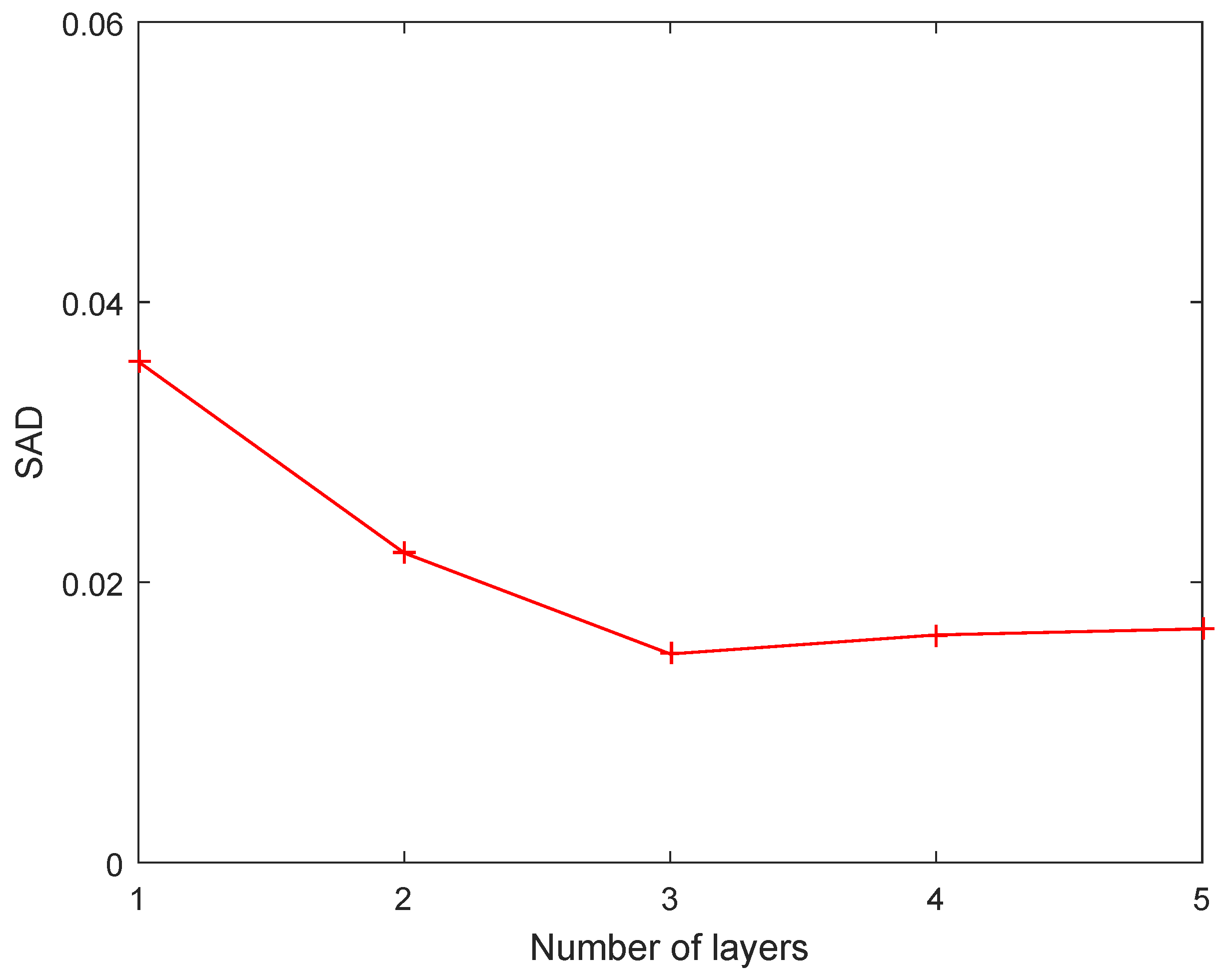
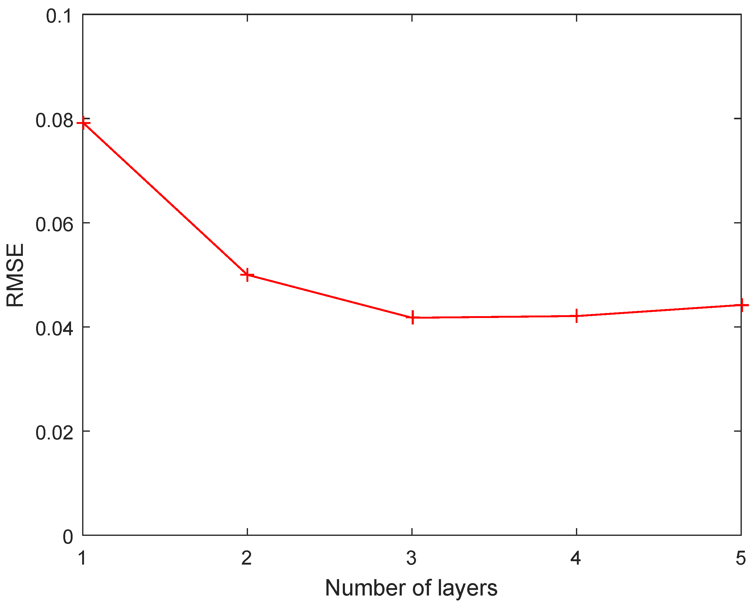
Vertex component analysis (VCA) [35] is utilized to initialize the matrix ${\mathbf{V}}_l$, and the fully constrained least squares (FCLS) algorithm [36] is utilized to initialize ${\mathbf{H}}_l$. Specifically, to avoid pixels with near-zero residues dominating the objective function, the maximum value in ${\mathbf{G}}_l$ and ${\mathbf{Q}}_l$ is limited to 100. As for the stopping criterion, the algorithm is stopped when the number of iterations reaches a preset maximum number $T_{\max }$ or the relative error $|{\mathcal{O}}^{(t+1)}-{\mathcal{O}}^{\left(t\right)}|/{\mathcal{O}}^{\left(t\right)}\le \epsilon$ is met. $T_{\max }$ is set to 500 and $\epsilon$ is set to ${10}^{-4}$ in this paper. Further, the parameters of the multi-layer structure in deep NMF-based methods are determined with reference to [31] through empirical examination. In Experiment 1, it is found that optimal performance is achieved when the number of layers L of the deep NMF structure is defined as 3. Therefore, we set L as 3 in the rest of the experiments.

3. Experiments

To verify the effectiveness of our method, several experiments are carried out on both synthetic and real HSI data. Seven HU methods, i.e., VCA-FCLS [35,36], ${\mathsf{\ell }}_{2,1}$-RNMF [16], DNMF [27], SDNMF-TV [31], CSsRS-NMF [18], MLNMF [25], and CANMF-TV [33] are compared to the proposed ${\mathsf{\ell }}_{2,1}$-RDNMF in the experiments. Two commonly utilized metrics, spectral angle distance (SAD) and root-mean-square error (RMSE), are used to quantify the performance of the obtained unmixing results [2].

3.1. Experiments on Synthetic Data

The used synthetic data are generated according to the methodology provided in [2]. The spectra used as endmembers are randomly assigned from the United States Geological Survey (USGS) digital spectral library [37]. The size of generated synthetic data is 100 × 100 pixels with 224 bands. To better simulate the real scenario, the synthetic data are contaminated by a possible complex noise composition involving dead pixels, Gaussian noise, and impulse noise. When adding the Gaussian noise, pixels’ values of the signal-to-noise ratio (SNR) are derived from ${\mathrm{SNR}}_{\mathrm{pixel}}\sim \mathcal{N}(\overline{\mathrm{SNR}},{\sigma }^2)$ with reference to [18]. To establish a reliable comparison, the reported results in the experiments are derived by averaging over 20 independent runs for each method. When the iteration number is set as 500, the time consumption of the proposed ${\mathsf{\ell }}_{2,1}$-RDNMF and other compared methods is presented in

Table 1. Time consumption of the proposed ${\mathsf{\ell }}_{2,1}$-RDNMF and other compared methods.

VCA-FCLS	${\mathsf{\ell }}_{2,1}$-NMF	DNMF	SDNMF-TV	CSsRS-NMF	MLNMF	CANMF-TV	${\mathsf{\ell }}_{2,1}$-RDNMF
1.30 s	9.51 s	20.72 s	141.60 s	123.80 s	21.82 s	149.63 s	57.06 s

.

3.1.1. Experiment 1 (Investigation of the Number of Layers)

The number of layers is a key parameter for a deep NMF-based method that determines the depth of the multi-layer structure and influences the unmixing performance. This experiment investigates the impact of different settings for the number of layers on the unmixing performance. The number of layers L is set as $1,2,3,\cdots ,6$. Figure 2 and Figure 3 display the SAD and RMSE results of ${\mathsf{\ell }}_{2,1}$-RDNMF under different settings of L. It can be observed that the two metrics show a similar trend when L varies. The performance of the multi-layer structure ($L\ge 2$) is superior to the single-layer structure ($L=1$), as expected. The metrics of endmembers and abundances both gradually improve with increasing L, and then, they degrade when L is larger than 3. In other words, optimal performance can be achieved by using a three-layer structure. Therefore, a three-layer structure is adopted in the rest of the experiments.

3.1.2. Experiment 2 (Investigation of Noise Intensities)

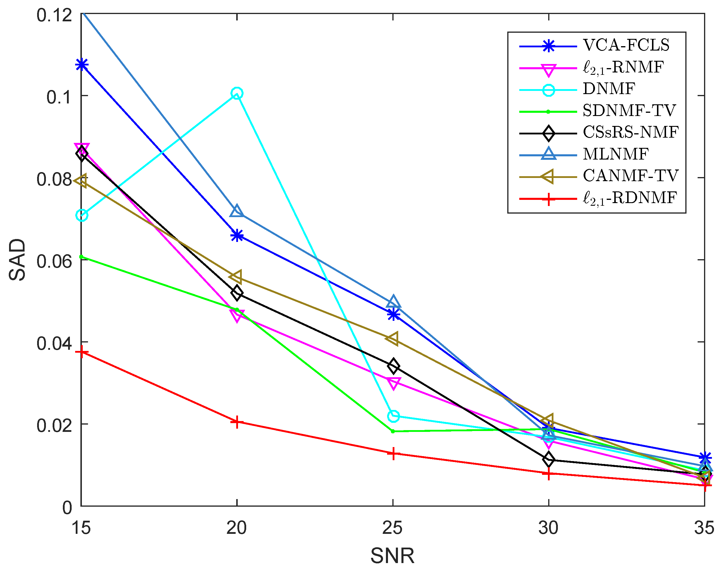
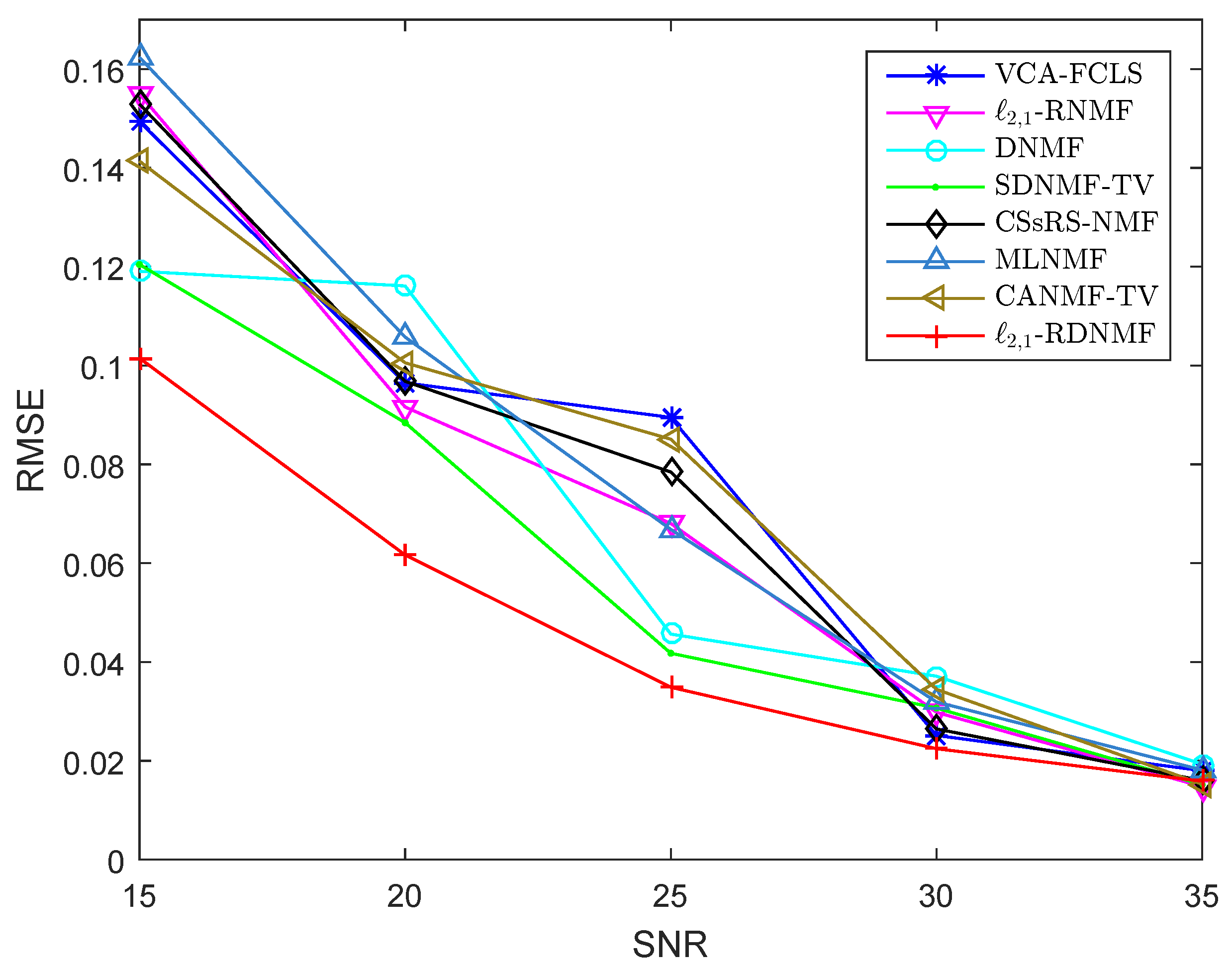
To verify the proposed method’s effectiveness, synthetic HSI data with various noise intensities are utilized to assess the algorithms’ performance. The value of $\overline{\mathrm{SNR}}$ is specified as 15, 20, 25, 30, or 35 in order to simulate various noise intensities; $\sigma$ is set to 5 in the experiment. Figure 4 and Figure 5 show the SAD and RMSE results of algorithms when the noise level varies. When ${\overline{\mathrm{SNR}}}_{\mathrm{pixel}}=35$, the algorithms all perform well and are at a comparable level. When the value of ${\overline{\mathrm{SNR}}}_{\mathrm{pixel}}$ decreases, all five methods’ performance degrades as anticipated. However, it can be seen that the proposed ${\mathsf{\ell }}_{2,1}$-RDNMF apparently obtains lower values of SAD and RMSE, which validates the robustness of ${\mathsf{\ell }}_{2,1}$-RDNMF to various noise levels.

3.1.3. Experiment 3 (Investigation of Noise Types)

The algorithms are also investigated on synthetic data with various forms of mixed noise added, which provides a better simulation of complicated mixed noise in real scenarios. The mixed noise is made up of a combination of dead pixels, Gaussian noise, and impulse noise. For the dead pixels, 0.5% of pixels are randomly selected to be dead pixels. For the Gaussian noise, ${\overline{\mathrm{SNR}}}_{\mathrm{pixel}}$ is set to 30. For the impulse noise, bands 30–40 are degraded by impulse noise with the noise density set to 0.05.

Table 2. SADs of different methods on synthetic data simulated with various types of noise. The best results are marked in bold.

Noise Type	Methods
	VCA-FCLS	${\mathsf{\ell }}_{2,1}$-NMF	DNMF	SDNMF-TV	CSsRS-NMF	MLNMF	CANMF-TV	${\mathsf{\ell }}_{2,1}$-RDNMF
Gaussian noise	0.0190	0.0159	0.0168	0.0187	0.0113	0.0172	0.0209	0.0080
Gaussian noise and Impulse noise	0.2006	0.2348	0.1635	0.1919	0.1466	0.3062	0.2078	0.0190
Gaussian noise and Dead pixels	0.2017	0.3170	0.2810	0.4668	0.5244	0.4296	0.5716	0.0233
Gaussian noise, Impulse noise, and Dead pixels	0.4721	0.5641	0.2865	0.4507	0.3660	0.5692	0.6282	0.0617

and

Table 3. RMSEs of different methods on synthetic data simulated with various types of noise. The best results are marked in bold.

Noise Type	Methods
	VCA-FCLS	${\mathsf{\ell }}_{2,1}$-NMF	DNMF	SDNMF-TV	CSsRS-NMF	MLNMF	CANMF-TV	${\mathsf{\ell }}_{2,1}$-RDNMF
Gaussian noise	0.0251	0.0298	0.0371	0.0307	0.0265	0.0319	0.0345	0.0225
Gaussian noise and Impulse noise	0.1719	0.1401	0.1060	0.1332	0.1780	0.1793	0.1256	0.0339
Gaussian noise and Dead pixels	0.3326	0.3330	0.2338	0.3165	0.4166	0.3804	0.3164	0.0441
Gaussian noise and Impulse noise and Dead pixels	0.4216	0.3737	0.2740	0.3411	0.4680	0.3222	0.3801	0.0522

report the SAD and RMSE results of algorithms under five types of noise situations, including Gaussian noise; Gaussian noise and impulse noise; Gaussian noise and dead pixels; and Gaussian noise, impulse noise, and dead pixels. The reported results show that ${\mathsf{\ell }}_{2,1}$-RDNMF achieves the best unmixing performance in the terms of endmembers and abundances under all four types of noise situations, which further confirms the robustness of the proposed ${\mathsf{\ell }}_{2,1}$-RDNMF under complicated mixed noise.

3.2. Experiments on Real Data

3.2.1. Samson Dataset

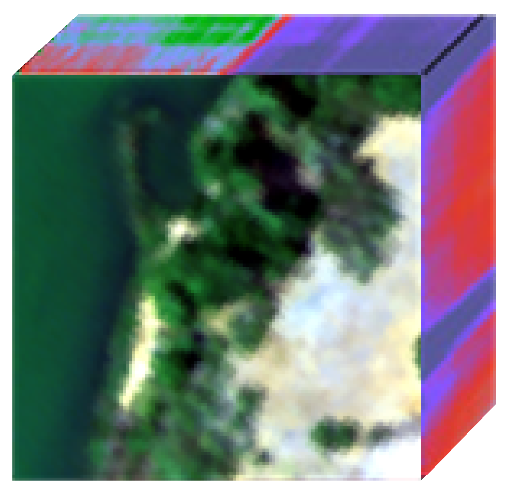
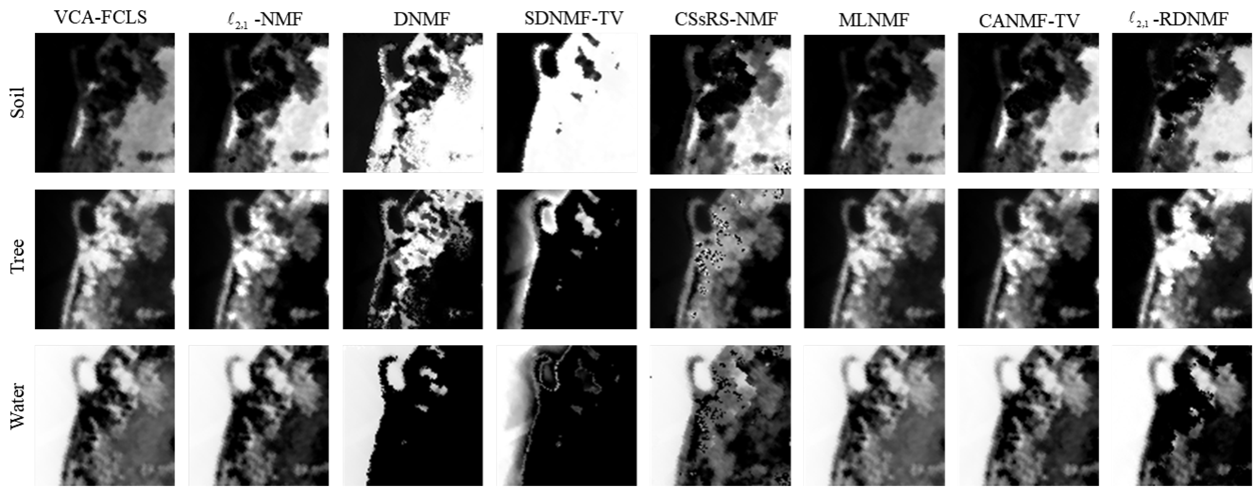
The first real HSI dataset used in our experiments is the Samson dataset [38], which contains 156 bands spanning the spectral range of 401 nm–889 nm. As shown in Figure 6, the used subscene consists of 95 × 95 pixels. Based on the previous studies in [31,39], there are three kinds of targets existing in the subscene, including water, trees, and soil.

Table 4. The SADs of algorithms on the Samson dataset. The best results are marked in bold.

Endmember	Methods
	VCA-FCLS	${\mathsf{\ell }}_{2,1}$-NMF	DNMF	SDNMF-TV	CSsRS-NMF	MLNMF	CANMF-TV	${\mathsf{\ell }}_{2,1}$-RDNMF
Soil	0.2680	0.1817	0.0568	0.1584	0.1675	0.1250	0.0903	0.0274
Tree	0.0518	0.0868	0.0524	0.1284	0.0870	0.0811	0.0625	0.0505
Water	0.1281	0.1235	0.1373	0.2076	0.2635	0.2492	0.1440	0.1467
Mean	0.1493	0.1307	0.0822	0.1648	0.1726	0.1518	0.0989	0.0748

presents the SAD results of the three targets achieved by the proposed ${\mathsf{\ell }}_{2,1}$-RDNMF and comparative methods. As the results show, ${\mathsf{\ell }}_{2,1}$-RDNMF outperforms the compared methods in all three targets and the mean value. Since the ground truth of abundances for the real dataset is unavailable, Figure 7 only displays the estimated abundance maps using the proposed ${\mathsf{\ell }}_{2,1}$-RDNMF. With comparison to the results presented in the previous works [31,39], the abundance maps are in accordance with the the reference maps.

3.2.2. Cuprite Dataset

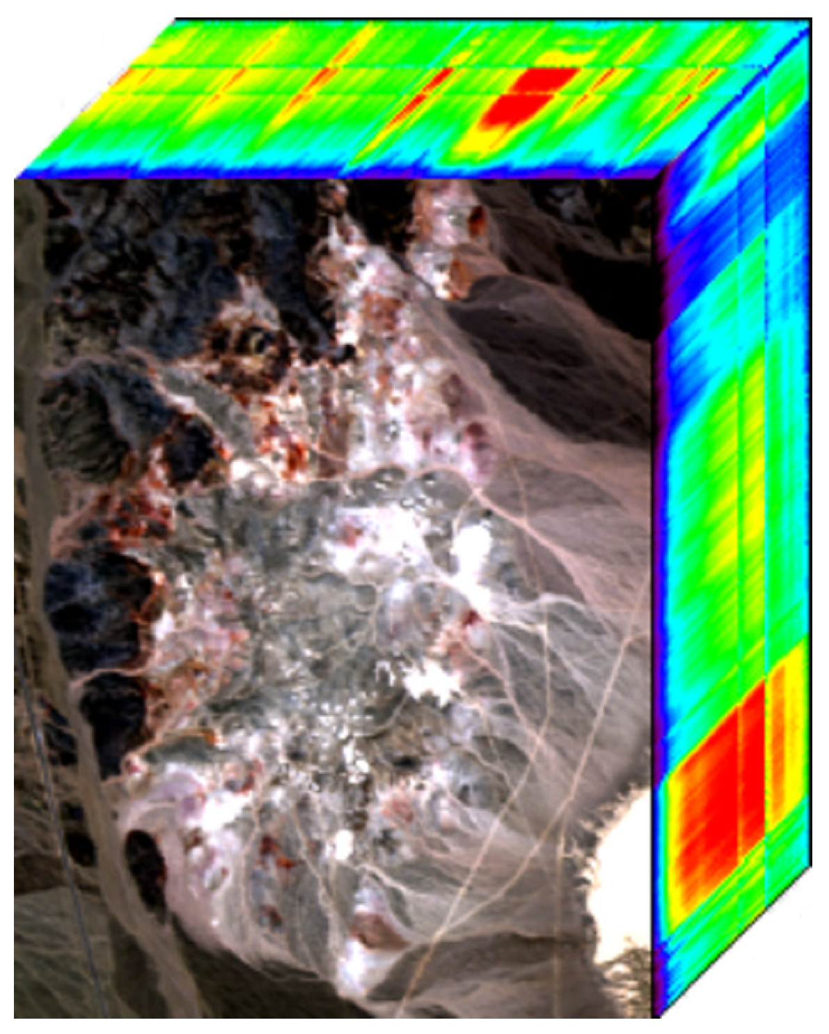
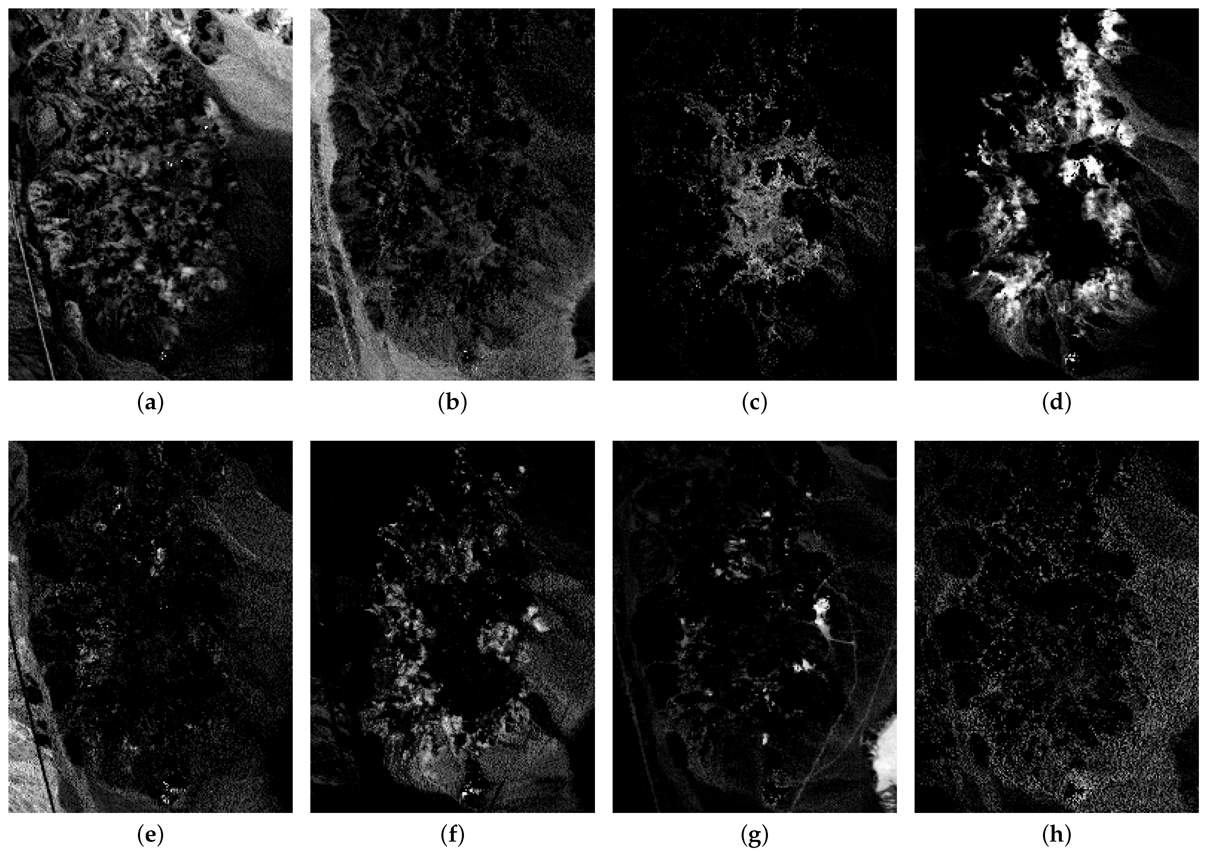
The second scene employed in the experiment is the Cuprite dataset collected by the AVIRIS sensor over a Cuprite area in Las Vegas, NV, US. As shown in Figure 8, the used subimage contains 250 × 191 pixels and 224 bands. After badly degraded bands (1–2, 76, 104–113, 148–167, and 221–224) are removed, there are 188 bands remaining that are used in the experiment.

Table 5. The SADs of algorithms on the Cuprite dataset. The best results are marked in bold.

Endmember	Methods
	VCA-FCLS	${\mathsf{\ell }}_{2,1}$-NMF	DNMF	SDNMF-TV	CSsRS-NMF	MLNMF	CANMF-TV	${\mathsf{\ell }}_{2,1}$-RDNMF
Alunite	0.0847	0.0968	0.0914	0.0917	0.0946	0.1567	0.1351	0.2765
Andradite	0.0778	0.0826	0.1084	0.0897	0.0831	0.1146	0.0781	0.0731
Buddingtonite	0.1215	0.1430	0.1115	0.1264	0.1224	0.1142	0.0601	0.1132
Dumortierite	0.1000	0.1329	0.1172	0.1323	0.1046	0.1648	0.1095	0.0821
Kaolinite #1	0.0855	0.0688	0.0629	0.0652	0.0738	0.0846	0.1504	0.0785
Kaolinite #2	0.1133	0.0888	0.0640	0.0613	0.0859	0.0941	0.1225	0.0599
Muscovite	0.1976	0.1349	0.2191	0.1532	0.1924	0.4113	0.1662	0.1216
Montmorillonite	0.1110	0.0632	0.0619	0.1276	0.0634	0.0665	0.0620	0.0637
Nontronite	0.0996	0.0982	0.1135	0.1227	0.0934	0.1382	0.1007	0.0833
Pyrope	0.1118	0.0583	0.1908	0.0573	0.0567	0.0787	0.0574	0.0524
Sphene	0.0544	0.2495	0.0545	0.2320	0.2506	0.0960	0.0898	0.0703
Chalcedony	0.1902	0.1242	0.1288	0.1283	0.1154	0.1525	0.1326	0.1464
Mean	0.1123	0.1118	0.1103	0.1156	0.1114	0.1393	0.1054	0.1017

presents the SAD results of the proposed ${\mathsf{\ell }}_{2,1}$-RDNMF and comparative methods on the Cuprite dataset. It can be observed that ${\mathsf{\ell }}_{2,1}$-RDNMF achieves the best performance in several minerals, including Andradite, Dumortierite, Kaolinite #2, Muscovite, Nontronite and Pyrope, as well as the mean value. Additionally, Figure 9 presents the abundance maps estimated by ${\mathsf{\ell }}_{2,1}$-RDNMF.

4. Conclusions

In this study, we provide an ${\mathsf{\ell }}_{2,1}$ norm-based robust deep NMF method (${\mathsf{\ell }}_{2,1}$-RDNMF) for HU. The ${\mathsf{\ell }}_{2,1}$ norms are effectively incorporated into two stages of the designed deep structure to achieve robustness to noise corruption in HU. Experiments conducted on synthetic data simulated with various noise intensities and types demonstrate that the proposed method possesses gratifying robustness to complex noise situations. Experiments conducted on real data also verify the effectiveness of our method.

References

1. Feng, X.R.; Li, H.C.; Wang, R.; Du, Q.; Jia, X.; Plaza, A.J. Hyperspectral unmixing based on nonnegative matrix factorization: A comprehensive review. IEEE J. Sel. Topics Appl. Earth Observ. Remote Sens. 2022, 15, 4414–4436. [Google Scholar] [CrossRef]
2. Qian, Y.; Jia, S.; Zhou, J.; Robles-Kelly, A. Hyperspectral unmixing via L1/2 sparsity-constrained nonnegative matrix factorization. IEEE Trans. Geosci. Remote Sens. 2011, 49, 4282–4297. [Google Scholar] [CrossRef] [Green Version]
3. Huck, A.; Guillaume, M.; Blanc-Talon, J. Minimum dispersion constrained nonnegative matrix factorization to unmix hyperspectral data. IEEE Trans. Geosci. Remote Sens. 2010, 48, 2590–2602. [Google Scholar] [CrossRef]
4. Lu, X.; Wu, H.; Yuan, Y.; Yan, P.; Li, X. Manifold regularized sparse NMF for hyperspectral unmixing. IEEE Trans. Geosci. Remote Sens. 2013, 51, 2815–2826. [Google Scholar] [CrossRef]
5. Wang, N.; Du, B.; Zhang, L. An endmember dissimilarity constrained non-negative matrix factorization method for hyperspectral unmixing. IEEE J. Sel. Top. Appl. Earth Observ. Remote Sens. 2013, 6, 554–569. [Google Scholar] [CrossRef]
6. Lei, T.; Zhou, J.; Qian, Y.; Xiao, B.; Gao, Y. Nonnegative-matrix-factorization-based hyperspectral unmixing with partially known endmembers. IEEE Trans. Geosci. Remote Sens. 2016, 54, 6531–6544. [Google Scholar]
7. Févotte, C.; Dobigeon, N. Nonlinear hyperspectral unmixing with robust nonnegative matrix factorization. IEEE Trans. Image Process. 2015, 24, 4810–4819. [Google Scholar] [CrossRef] [Green Version]
8. Li, C.; Ma, Y.; Mei, X.; Liu, C.; Ma, J. Hyperspectral unmixing with robust collaborative sparse regression. Remote Sens. 2016, 8, 588. [Google Scholar] [CrossRef] [Green Version]
9. He, W.; Zhang, H.; Zhang, L. Sparsity-regularized robust non-negative matrix factorization for hyperspectral unmixing. IEEE J. Sel. Top. Appl. Earth Observ. Remote Sens. 2016, 9, 4267–4279. [Google Scholar] [CrossRef]
10. Ding, C.; Zhou, D.; He, X.; Zha, H. R1-PCA: Rotational invariant L1-norm principal component analysis for robust subspace factorization. In Proceedings of the 23rd International Conference on Machine Learning, Pittsburgh, PA, USA, 25–29 June 2006; pp. 281–288. [Google Scholar]
11. Nie, F.; Huang, H.; Cai, X.; Ding, C.H. Efficient and robust feature selection via joint 2,1-norms minimization. In Advances in Neural Information Processing Systems 23 (NIPS 2010); Morgan Kaufmann: Vancouver, BC, Canada, 2010; pp. 1813–1821. [Google Scholar]
12. Huang, H.; Ding, C. Robust tensor factorization using R1 norm. In Proceedings of the 2008 IEEE Conference on Computer Vision and Pattern Recognition (CVPR), Anchorage, AK, USA, 23–28 June 2008; IEEE: Piscataway, NJ, USA, 2008; pp. 1–8. [Google Scholar]
13. Ren, C.X.; Dai, D.Q.; Yan, H. Robust classification using 2,1-norm based regression model. Pattern Recognit. 2012, 45, 2708–2718. [Google Scholar] [CrossRef]
14. Yang, S.; Hou, C.; Zhang, C.; Wu, Y. Robust non-negative matrix factorization via joint sparse and graph regularization for transfer learning. Neur. Comput. Appl. 2013, 23, 541–559. [Google Scholar] [CrossRef]
15. Ma, Y.; Li, C.; Mei, X.; Liu, C.; Ma, J. Robust sparse hyperspectral unmixing with 2,1 norm. IEEE Trans. Geosci. Remote Sens. 2017, 55, 1227–1239. [Google Scholar] [CrossRef]
16. Kong, D.; Ding, C.; Huang, H. Robust nonnegative matrix factorization using L21-norm. In Proceedings of the 20th ACM International Conference on Information and Knowledge Management, Glasgow, UK, 24–28 October 2011; ACM: New York, NY, USA, 2011; pp. 673–682. [Google Scholar]
17. Wang, Y.; Pan, C.; Xiang, S.; Zhu, F. Robust hyperspectral unmixing with correntropy-based metric. IEEE Trans. Image Process. 2015, 24, 4027–4040. [Google Scholar] [PubMed]
18. Li, X.; Huang, R.; Zhao, L. Correntropy-based spatial-spectral robust sparsity-regularized hyperspectral unmixing. IEEE Trans. Geosci. Remote Sens. 2020, 59, 1453–1471. [Google Scholar] [CrossRef]
19. Wang, H.; Yang, W.; Guan, N. Cauchy sparse NMF with manifold regularization: A robust method for hyperspectral unmixing. Knowl.-Based Syst. 2019, 184, 104898. [Google Scholar] [CrossRef]
20. Huang, R.; Li, X.; Zhao, L. Spectral-spatial robust nonnegative matrix factorization for hyperspectral unmixing. IEEE Trans. Geosci. Remote Sens. 2019, 57, 8235–8254. [Google Scholar] [CrossRef]
21. Peng, J.; Zhou, Y.; Sun, W.; Du, Q.; Xia, L. Self-paced nonnegative matrix factorization for hyperspectral unmixing. IEEE Trans. Geosci. Remote Sens. 2021, 59, 1501–1515. [Google Scholar] [CrossRef]
22. Zheng, Q.; Zhao, P.; Li, Y.; Wang, H.; Yang, Y. Spectrum interference-based two-level data augmentation method in deep learning for automatic modulation classification. Neur. Comput. Appl. 2021, 33, 7723–7745. [Google Scholar]
23. Zhao, M.; Liu, Q.; Jha, A.; Deng, R.; Yao, T.; Mahadevan-Jansen, A.; Tyska, M.J.; Millis, B.A.; Huo, Y. VoxelEmbed: 3D instance segmentation and tracking with voxel embedding based deep learning. In Proceedings of the Machine Learning in Medical Imaging: 12th International Workshop, MLMI 2021, Held in Conjunction with MICCAI 2021, Strasbourg, France, 27 September 2021, Proceedings 12; Springer: Berlin/Heidelberg, Germany, 2021; pp. 437–446. [Google Scholar]
24. Rajabi, R.; Ghassemian, H. Spectral unmixing of hyperspectral imagery using multilayer NMF. IEEE Geosci. Remote Sens. Lett. 2014, 12, 38–42. [Google Scholar]
25. Cichocki, A.; Zdunek, R. Multilayer nonnegative matrix factorisation. Electron. Lett. 2006, 42, 947–948. [Google Scholar] [CrossRef] [Green Version]
26. De Handschutter, P.; Gillis, N.; Siebert, X. A survey on deep matrix factorizations. Comput. Sci. Rev. 2021, 42, 100423. [Google Scholar] [CrossRef]
27. Trigeorgis, G.; Bousmalis, K.; Zafeiriou, S.; Schuller, B.W. A deep matrix factorization method for learning attribute representations. IEEE Trans. Patt. Anal. Mach. Intell. 2016, 39, 417–429. [Google Scholar] [CrossRef] [PubMed] [Green Version]
28. Chen, W.S.; Zeng, Q.; Pan, B. A survey of deep nonnegative matrix factorization. Neurocomputing 2022, 491, 305–320. [Google Scholar] [CrossRef]
29. Sun, J.; Kong, Q.; Xu, Z. Deep alternating non-negative matrix factorisation. Knowl.-Based Syst. 2022, 251, 109210. [Google Scholar] [CrossRef]
30. Fang, H.; Li, A.; Xu, H.; Wang, T. Sparsity-constrained deep nonnegative matrix factorization for hyperspectral unmixing. IEEE Geosci. Remote Sens. Lett. 2018, 15, 1105–1109. [Google Scholar] [CrossRef]
31. Feng, X.R.; Li, H.C.; Li, J.; Du, Q.; Plaza, A.; Emery, W.J. Hyperspectral unmixing using sparsity-constrained deep nonnegative matrix factorization with total variation. IEEE Trans. Geosci. Remote Sens. 2018, 56, 6245–6257. [Google Scholar] [CrossRef]
32. Huang, R.; Li, X.; Fang, Y.; Cao, Z.; Xia, C. Robust Hyperspectral Unmixing with Practical Learning-Based Hyperspectral Image Denoising. Remote Sens. 2023, 15, 1058. [Google Scholar] [CrossRef]
33. Feng, X.R.; Li, H.C.; Liu, S.; Zhang, H. Correntropy-based autoencoder-like NMF with total variation for hyperspectral unmixing. IEEE Trans. Geosci. Remote Sens. 2022, 19, 1–5. [Google Scholar]
34. Lee, D.D.; Seung, H.S. Algorithms for non-negative matrix factorization. In Advances in Neural Information Processing Systems 13 (NIPS 2000); Morgan Kaufmann: Denver, CO, USA, 2001; pp. 556–562. [Google Scholar]
35. Nascimento, J.M.; Dias, J.M. Vertex component analysis: A fast algorithm to unmix hyperspectral data. IEEE Trans. Geosci. Remote Sens. 2005, 43, 898–910. [Google Scholar] [CrossRef] [Green Version]
36. Heinz, D.C.; Chang, C.I. Fully constrained least squares linear spectral mixture analysis method for material quantification in hyperspectral imagery. IEEE Trans. Geosci. Remote Sens. 2001, 39, 529–545. [Google Scholar] [CrossRef] [Green Version]
37. Clark, R.N.; Swayze, G.A.; Gallagher, A.J.; King, T.V.; Calvin, W.M. The US Geological Survey, Digital Spectral Library: Version 1 (0.2 to 3.0 um); U.S. Geological Survey Open-File ReportThe US Geological Survey: Denver, CO, USA, 1993. [Google Scholar]
38. Zhu, F. Hyperspectral Unmixing Datasets & Ground Truths. 2014. Available online: http://www.escience.cn/people/feiyunZHU/Dataset_GT.html (accessed on 10 March 2019).
39. Zhu, F.; Wang, Y.; Fan, B.; Xiang, S.; Meng, G.; Pan, C. Spectral unmixing via data-guided sparsity. IEEE Trans. Image Process. 2014, 23, 5412–5427. [Google Scholar] [CrossRef] [PubMed] [Green Version]
Figure 1. Schematic diagram of deep NMF.
Remotesensing 15 02900 g001
Figure 2. SAD results of proposed 2 , 1 -RDNMF with different settings of the number of layers.
Remotesensing 15 02900 g002
Figure 3. RMSE results of proposed 2 , 1 -RDNMF with different settings of the number of layers.
Remotesensing 15 02900 g003
Figure 4. SAD results of different methods on data simulated with various intensities of Gaussian noise.
Remotesensing 15 02900 g004
Figure 5. RMSE results of different methods on data simulated with various intensities of Gaussian noise.
Remotesensing 15 02900 g005
Figure 6. The Samson dataset used in the experiment.
Remotesensing 15 02900 g006
Figure 7. Abundance maps estimated using 2 , 1 -RDNMF on the Samson dataset.
Remotesensing 15 02900 g007
Figure 8. The Cuprite dataset used in the experiment.
Remotesensing 15 02900 g008
Figure 9. Abundance maps estimated by 2 , 1 -RDNMF on the Cuprite dataset. (a) Alunite. (b) Andradite. (c) Buddingtonite. (d) Dumortierite. (e) Kaolinite #1. (f) Kaolinite #2. (g) Muscovite. (h) Montmorillonite. (i) Nontronite. (j) Pyrope. (k) Sphene. (l) Chalcedony.
Remotesensing 15 02900 g009aRemotesensing 15 02900 g009b