A Multi-Attention Autoencoder for Hyperspectral Unmixing Based on the Extended Linear Mixing Model

Abstract

Hyperspectral unmixing, which decomposes mixed pixels into the endmembers and corresponding abundances, is an important image process for the further application of hyperspectral images (HSIs). Lately, the unmixing problem has been solved using deep learning techniques, particularly autoencoders (AEs). However, the majority of them are based on the simple linear mixing model (LMM), which disregards the spectral variability of endmembers in different pixels. In this article, we present a multi-attention AE network (MAAENet) based on the extended LMM to address the issue of the spectral variability problem in real scenes. Moreover, the majority of AE networks ignore the global spatial information in HSIs and operate pixel- or patch-wise. We employ attention mechanisms to design a spatial–spectral attention (SSA) module that can deal with the band redundancy in HSIs and extract global spatial features through spectral correlation. Moreover, noticing that the mixed pixels are always present in the intersection of different materials, a novel sparse constraint based on spatial homogeneity is designed to constrain the abundance and abstract local spatial features. Ablation experiments are conducted to verify the effectiveness of the proposed AE structure, SSA module, and sparse constraint. The proposed method is compared with several state-of-the-art unmixing methods and exhibits competitiveness on both synthetic and real datasets.

1. Introduction

Hyperspectral images (HSIs) have both spatial and spectral information. In particular, hundreds of spectral bands can reflect the physical characteristics of objects, which can greatly enhance the ability in various remote sensing applications, i.e., environmental monitoring, resource exploration, and target detection and recognition [1].

Due to the tradeoff between the spatial and spectral resolutions, the spatial resolutions of hyperspectral sensors are limited. Consequently, HSIs contain mixed pixels, which contain multiple materials. The presence of mixed pixels reduces the performance of HSI analysis for further applications. Therefore, a variety of spectral mixing models and spectral unmixing algorithms have been proposed to decompose mixed pixels into a set of pure spectra (denoted endmembers) and their corresponding proportions (denoted abundances). In general, the hyperspectral unmixing process mainly contains two parts, endmember extraction and abundance estimation. The endmember extraction finds the spectra of all kinds of materials in the scene, while the abundance estimation determines the fraction of endmembers contained in each pixel.

An unmixing algorithm is based on a certain spectral mixing model. The spectral mixing models can be divided into the linear mixing model (LMM) and the nonlinear mixing model (NLMM) [2]. The LMM assumes that the signal obtained by the spectrometer is a direct reflection of incident light on the material, and the mixing spectra are a linear combination of the various endmembers’ spectra. In contrast, NLMMs [3] make the assumption that the scattering of photons takes place on multiple materials in the scene. The complex assumptions of nonlinear models are made for specific conditions and require a great deal of prior knowledge. Therefore, LMM is the most widely used because of its strong generalization ability in remote sensing and clear physical significance.

However, the illumination variations and atmospheric conditions may cause the spectra of endmembers to vary within an image, which is called spectral variability. The unmixing results of LMM will be degraded due to the spectral variability issue. Therefore, various methods have been developed to mitigate the impacts of spectral variability in spectral unmixing. The unmixing methods, which take the spectral variability into consideration, can be divided into two categories, the endmember-bundle-based approaches and the parametric endmember models. The endmember-bundle-based approaches [4,5,6] generate a bundle of spectra for each endmember from the input data and explore which spectrum of each endmember bundle is the best to generate the combination of each pixel. The parametric models [7,8,9,10,11], such as the extended LMM (ELMM) [7], the perturbed LMM (PLMM) [9], and the generalized LMM (GLMM) [11], introduce extra parameters into the traditional LMM to simulate the spectral variability. The ELMM individually scales each endmember in a pixel by a constant factor. Even more, each band of each endmember spectrum is given its own scaling factor in the GLMM. Considering the computational complexity, we choose the ELMM to model the spectral variability in our method.

According to the development of the unmixing problem, the existing linear unmixing methods can be divided into three types: supervised, semisupervised, and unsupervised methods.

The supervised unmixing algorithms generally consist of two steps. They need to extract the endmembers as a prior first and then solve the abundance. The endmember extraction methods can be divided into two categories according to the pure pixel assumption. If pure pixels for each material exist in the image, the endmembers are located at the vertices of the HSI data simplex based on LMM. Algorithms such as vertex component analysis (VCA) [12], Nfindr [13], and pixel purity exponent (PPI) [14] were proposed to find these vertices. If there is no pure pixel in the scene, appropriate expansions of the HSI data simplex are conducted, such as minimum volume simplex analysis (MVSA) [15] and iterative constrained endmember (ICE) [16]. Later, some abundance-estimation algorithms such as fully constrained least square (FCLS) [17,18] are used to complete the unmixing process. Since these supervised methods separate endmember extraction and abundance estimation, the abundance results of unmixing largely depend on the accuracy of the extracted endmembers.

The semisupervised methods [19,20,21] are spare regression unmixing methods based on the existing complete spectral library. They convert the spectral unmixing problem into selecting the optimal linear combination of spectra subset in the library. Nevertheless, because of the redundancy of the spectral library and the spectral variability of the endmembers, it is difficult to find the perfect match of endmembers in the spectral library.

The unsupervised methods [22,23,24,25,26,27,28,29,30,31,32] are blind-source separation algorithms that decompose the HSI matrix into the endmember matrix and abundance matrix simultaneously, such as independent component analysis (ICA) [28], non-negative matrix factorization (NMF), non-negative tensor factorization (NTF) unmixing algorithms, and some deep learning methods. However, because the objective function used in the optimization is non-convex, it is easy to fall into the local minimum, and the unmixing result may be unstable. Therefore, in order to achieve better performance, different regularizations have been appended to the objective function to improve the performance [23,24,25,29,30].

In recent years, spectral unmixing methods based on deep learning have become increasingly popular with researchers. The most widely concerned is the autoencoder (AE) framework, through which unsupervised spectral unmixing can be performed [33,34,35]. An AE framework generally consists of an encoder and a decoder. The encoder transforms the input HSIs into a hidden layer containing low-dimensional embedding, which corresponds to the abundance. The decoder is constructed on a certain mixing model with the corresponding endmember matrix as another input. Generally, it is a simple linear layer without bias whose weight is the endmember matrix.

Palsson et al. [36] studied the structure and loss function of autoencoders used for spectral unmixing systematically for the first time. It was shown that the spectral angle distance (SAD) may be a more suitable loss function and deeper encoders do not always give better results. To achieve a robust unmixing performance by AE in the presence of outliers, some denoising AEs [37,38] have been proposed, such as DAEN presented by Su et al. [39], which consists of stacked AEs for initializing endmembers and a variational AE to optimize the results. Nevertheless, these AE networks used fully-connected layers as the base structure in the encoder part, so the spatial information in the image was ignored. Palsson et al. [40] introduced the convolutional neural network (CNN) into the AE unmixing methods. The advantage of CNN is exploiting the neighbor information of pixels [41,42]. As a kind of unsupervised unmixing network, more prior knowledge is added into the loss function to avoid a local minimum, such as a sparsity or smoothing constraint on the abundance [43,44] or a minimum volume constraint on the endmembers [45,46].

Most recently, more innovations have been focused on the structure of the encoder. Hong et al. [47] proposed an endmember-guided unmixing network (EGU-Net) that included a Siamese network to learn the endmember features from pure or nearly-pure pixels and then share the weight with the main encoder. Xu et al. [44] proposed an AE with global–local smoothing. It contained two modules, the local continuous conditional random field smoothing module and the global recurrent smoothing module, which exploit local and global spatial features, respectively. However, these networks were limited to the encoder part and ignored the decoder which could have a more complicated fitting capability for the reconstruction of HSIs. In [48], Shi et al. proposed the probabilistic generative model for spectral unmixing (PGMSU), which uses a variational AE framework to generate an arbitrary posterior distribution of endmembers for each material of each pixel. Li et al. [49] used 3D-CNN combined with a channel attention network to solve the unmixing problem. Zhao et al. [50] proposed an unmixing AE that used 3D-CNN as a basic structure to integrate the spectral information and introduced spectral variability into the decoder.

As we can see from the discussion above, most unmixing AEs ignore the global information of HSIs. In the natural scene, the spectral similarity between long-range pixels is common, which is not considered by the pixel-wise or patch-wise AEs. Meanwhile, the spectral variability caused by illumination and shadow should be considered. The simple decoders based on LMM cannot fully exploit the powerful representation ability of encoders. Moreover, the unsupervised unmixing problem is still ill-posed after all. The initialization of the networks will partly influence the result. Currently, most endmember matrices of unmixing AEs are initialized with VCA or randomly [35]. The inappropriate initialized weights may make the unmixing results unstable or trap them in a local minimum.

In this article, we propose an unsupervised hyperspectral unmixing method based on a multi-attention AE network (MAAENet). We introduce the spectral variability model into the decoder based on ELMM, which improves the unmixing performance further. In the encoder, we design a module based on an attention mechanism called spectral–spatial attention (SSA) module that can help the encoder compute the importance of each spectral channel and gather spatial information globally. Meanwhile, we propose an abundance-regularization term based on spatial homogeneity to exploit the local spatial features of each pixel. In addition, we use a more stable endmember initialization method to avoid local minima as much as possible.

The main contributions of this article are summarized as follows:

• A novel AE architecture based on the ELMM is proposed for spectral unmixing. The decoder is specifically designed to deal with the spectral variability by adding pixel-wise scaling factors of the endmembers in real scenes.
• A spatial–spectral attention (SSA) module is designed by incorporating a non-local attention mechanism and a spectral attention mechanism to extract the spatial–spectral features of HSIs effectively. The non-local attention mechanism exploits the global spatial feature of pixels.
• A flexible constraint to abundance is proposed as a regularization called ${\mathcal{L}}_{\mathrm{SHC}}$. The relationship between the mixing severity and spatial homogeneity is considered in ${\mathcal{L}}_{\mathrm{SHC}}$ as local spatial prior knowledge.

This article is organized as follows. Section 2 briefly reviews the LMM and extended LMM. Section 3 describes the proposed unmixing AE framework, including the network architecture, the structure of the SSA module, and the loss function. Section 4 is the experimental section. Finally, the conclusions of our work are presented in Section 5.

2. Problem Formulation

2.1. Linear Mixing Model

The hyperspectral data is denoted $\mathbf{Y}=\left[{\mathbf{y}}_1,{\mathbf{y}}_2,\dots ,{\mathbf{y}}_n\right]\in {\mathbb{R}}^{b\times n}$, where b denotes the number of bands, $n=h\times w$ is the number of pixels, and h and w are the numbers of image rows and columns, respectively. The goal of spectral unmixing is to estimate the spectral vector ${\mathbf{e}}_p$ of all the endmembers contained in the image and the abundance vector ${\mathbf{a}}_n$ of these endmembers in each pixel. The endmember spectrum matrix of the HSI is denoted $\mathbf{E}=[{\mathbf{e}}_1,{\mathbf{e}}_2,\dots ,{\mathbf{e}}_p]\in {\mathbb{R}}^{b\times p}$, and $\mathbf{A}=[{\mathbf{a}}_1,{\mathbf{a}}_2,\dots ,{\mathbf{a}}_n]\in {\mathbb{R}}^{p\times n}$ is the abundance matrix of all the pixels, where p is the number of endmembers. According to the LMM of hyperspectral unmixing, the spectra $\mathbf{Y}$ in the image can be expressed as:

$$\mathbf{Y}=\mathbf{EA}+\mathbf{N}$$

(1)

where $\mathbf{N}\in {\mathbb{R}}^{b\times n}$ is the additive noise. Two constraints are applied to the abundance coefficients. One is the abundance non-negative constraint (ANC), which requires the abundance coefficients to be non-negative. The other is the abundance sum-to-one constraint (ASC), since the spectra of an arbitrary pixel should be completely represented by the contributions of the endmembers. These two constraints are given by the following equations:

$$\begin{array}{c}\mathrm{ANC}:\mathbf{A}\ge \mathbf{0}\\ \mathrm{ASC}:{\mathbf{1}}_p\mathbf{A}={\mathbf{1}}_n\end{array}$$

(2)

where ${\mathbf{1}}_p\in {\mathbb{R}}^{1\times p}$ and ${\mathbf{1}}_n\in {\mathbb{R}}^{1\times n}$ represent all-one row vectors.

2.2. Extended Linear Mixing Model

The LMM, as a simplified model for spectral unmixing, cannot adapt to natural scenes well. In reality, the variation in atmospheric, illumination, and environmental conditions causes spectral variability [51], which means there may be multiple spectra of the same material in the image. Various models that adopt additional parameters based on the LMM have been proposed to address the spectral variability of endmembers in unmixing problems, such as augmented LMM [8], perturbed LMM [9], and extended LMM [7,10].

In this research, we implement the ELMM into the proposed unmixing network architecture to address the endmember variability. The ELMM employs scaling factors to approximate the variation of each endmember, which can be formulated as:

$${\mathbf{y}}_k=\mathbf{E}{\mathbf{s}}_k{\mathbf{a}}_k+{\mathbf{n}}_k$$

(3)

where ${\mathbf{s}}_k\in R^{p\times p}$ is a diagonal matrix with non-negative diagonal elements. The diagonal elements of ${\mathbf{s}}_k$ are scaling coefficients representing the spectral variability caused by the atmosphere and shading in the actual scene. The ELMM for all the pixels can be rewritten as following in matrix form:

$$\mathbf{Y}=\mathbf{E}\left(\mathbf{S}\odot \mathbf{A}\right)+\mathbf{N}$$

(4)

where $\mathbf{S}\in {\mathbb{R}}^{p\times n}$ is an incorporation of ${\mathbf{s}}_k$ for all pixels and its kth column consists of the diagonal elements of ${\mathbf{s}}_k$. The mathematical symbol ⊙ denotes the Hadamard product.

3. Proposed Method

In this section, we detail the proposed unmixing method. The proposed unmixing network includes two main parts, namely, the encoder and the decoder. The encoder is designed to learn the low-dimension spectra representation and potential spatial–spectral features of the input HSI. The last layer of the encoder is the learned abundance map $\widehat{\mathbf{A}}$, which can be expressed as:

$$\widehat{\mathbf{A}}={\mathcal{G}}_E\left(\mathbf{Y}\right)$$

(5)

where ${\mathcal{G}}_E(•)$ denotes the nonlinear mapping function learned by the encoder. The overall structure of the encoder is shown in Figure 1. Convolution layers are used as the basic layers to exploit the information of the hyperspectral data cube. The first layer is a 3 × 3 Conv layer used to integrate the neighborhood features of each pixel. After that, there is a spatial–spectral attention module that is specially designed to extract the spatial and spectral features. A detailed description of the SSA module is in Section 3.1. The next two layers use a 1 × 1 Conv kernel and LeakyReLU activation function to map the features into low-dimensional features. The last layer uses a 1 × 1 Conv kernel to compress the features to the abundance vectors, and the softmax function is used as an activation function to satisfy ANC and ASC.

Furthermore, a 3 × 3 Conv layer is followed by a normalization function to apply a sparse regularization on abundance. More details on this regularization are given in Section 3.2.

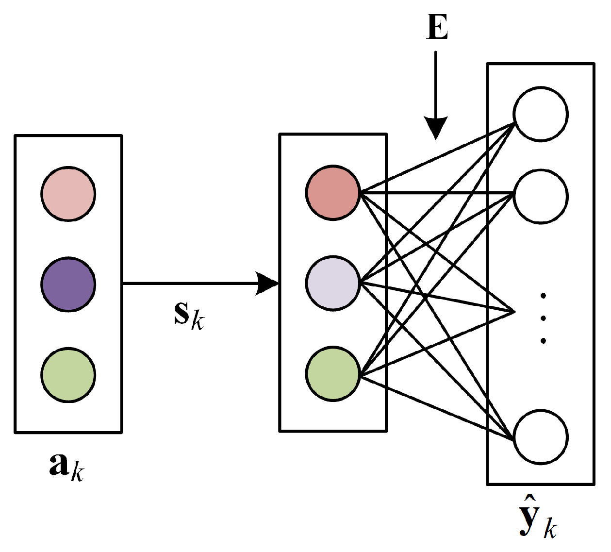
The decoder of the proposed network architecture is designed strictly according to the ELMM. The decoding function ${\mathcal{G}}_D(•)$ of the reconstruction process can be formulated as:

$$\widehat{\mathbf{Y}}={\mathcal{G}}_D\left(\mathbf{A}\right)=\mathbf{E}\left(\mathbf{S}\odot \mathbf{A}\right)$$

(6)

The weight of the decoder is an endmember matrix and the output is the reconstructed HSI $\widehat{\mathbf{Y}}$. Most decoders of unmixing AEs [36,37,38,39] are based on the simple LMM, which could waste the powerful ability of encoders to extract features. In this research, we introduce the ELMM into our decoder to enhance the fitting ability of the decoder. As shown in Figure 1, the decoder needs two parameter matrices: the scaling factor matrix $\mathbf{S}$ and the endmember matrix $\mathbf{E}$. The detailed reconstruction process of the kth pixel in the HSI is shown in Figure 2. According to the formulation of the ELMM given by Equation (3), the scaling factor ${\mathbf{s}}_k$ is applied to the abundance vector ${\mathbf{a}}_k$ to simulate the spectral variability of each endmember. The values of the diagonal elements of ${\mathbf{s}}_k$ are all initialized as 1, which represents the situation with no spectral variability. Then, the scaled abundance vector is input to a dense layer to reconstruct the pixel spectra, where the weights are correlated with the endmembers. The weights of the decoder are initialized using the endmembers extracted with the method detailed in Section 4.2 and the reflectance of each band is limited to the range of 0 to 1 in the optimization process.

3.1. Spatial–Spectral Attention (SSA) Module

HSIs have rich spatial information and spectral information. Normally, the convolution layers of the networks can only extract features within the local neighborhood and ignore the global information of input. Moreover, HSIs have hundreds of bands and some of them are highly correlated, which means some bands may be redundant. Thus, giving different weights to each band according to their importance can strengthen the fitting ability of networks. Recently, various attention mechanisms have been proposed for computer-vision tasks [52,53,54,55]. The attention mechanisms can be regarded as reweighting processes, which allow the networks efficiently to divert attention to the most important regions of the input data and disregard the irrelevant parts.

In this research, we construct an attention module called the spatial–spectral attention (SSA) module for the encoder network. As shown in Figure 3, the SSA module consists of two branches, a non-local attention module for extracting global spatial correlation information and a spectral attention module for weighting the importance of the spectral information in each band.

The non-local operation aims to build the connection between a single pixel and all the other pixels. In a natural scene, similar pixels, which have similar spectra, exist not only in the neighborhood but also in long-distance regions. In addition, pixels with similar spectra are likely to have the same abundance of endmembers. It is helpful to extract global information for solving the unmixing problem. Therefore, we proposed a non-local attention module that can capture global information by computing the relationship between any two positions. Different from the non-local neural network proposed in [54], in our method, we made some modifications to make the module more suitable for applications in HSIs with a clear physical interpretation. Since each pixel of an HSI has its own spectrum, we adopt the spectral correlation instead of the dot product used in [54] to define the pairwise function for computing the similarity in the embedding space. The function $f(•)$ is given as:

$$f({\mathbf{x}}_i,{\mathbf{x}}_j)=\frac{{{\mathbf{x}}_i}^{\mathrm{T}}{\mathbf{x}}_j}{∥{\mathbf{x}}_i∥∥{\mathbf{x}}_j∥}$$

(7)

where ${\mathbf{x}}_i$ and ${\mathbf{x}}_j$ are the spectral features of the ith pixel and jth pixel, respectively.

We wrap this operation into the non-local architecture illustrated in Figure 3. The specific operations are as follows. Let $\mathbf{X}\in {\mathbb{R}}^{c\times h\times w}$ denote the input feature map with c channels. First, feature transformation is performed by two Conv layers with a convolution kernel size of 1 × 1, and the output is $\{{\mathbf{X}}_1,{\mathbf{X}}_2\}\in {\mathbb{R}}^{c\times h\times w}$. Then, unfold ${\mathbf{X}}_1,{\mathbf{X}}_2$ by pixels and obtain $\{\mathbf{U},\mathbf{V}\}\in {\mathbb{R}}^{c\times n}$. After that, the non-local similarity map ${\mathbf{W}}_n\in {\mathbb{R}}^{n\times n}$, which denotes the similarity between the feature vector of each pixel, is formulated as follows:

$${\mathbf{W}}_n(i,j)=\frac{e^{f({\mathbf{U}}_i,{\mathbf{V}}_j)}}{{\displaystyle \sum _{i=1}^n}{e}^{f({\mathbf{U}}_i,{\mathbf{V}}_j)}}$$

(8)

where ${\mathbf{U}}_i$ is the ith column of $\mathbf{U}$ and ${\mathbf{V}}_j$ is the jth column of $\mathbf{W}$. The element ${\mathbf{W}}_n(i,j)$ denotes the globally normalized spectral similarity between the ith pixel in ${\mathbf{X}}_1$ and the jth pixel in ${\mathbf{X}}_2$. Thus, each pixel is associated with all the other pixels through ${\mathbf{W}}_n$. Finally, the flattened $\mathbf{X}$ is multiplied by ${\mathbf{W}}_n$ to obtain ${\mathbf{X}}_{\mathrm{NS}}$, which contains the global spatial correlation information.

Another branch is the spectral attention module, which is a kind of channel attention mechanism. The spectral attention module is designed to obtain the weights to describe the importance of all spectral bands. The representational power of the network can be improved by dynamically adjusting the weight of each band. The specific operations are as follows. First, the input feature map is sent to a convolution layer to integrate the information of all channels, and the output is denoted as ${\mathbf{X}}_3\in {\mathbb{R}}^{c\times h\times w}$. Then, mean pooling and standard deviation pooling of each channel are conducted separately to obtain the spectral features. The formulas of ${\mathbf{W}}_{\mathrm{mean}}\in {\mathbb{R}}^c$ and ${\mathbf{W}}_{\mathrm{std}}\in {\mathbb{R}}^c$ are given as follows:

$${\mathbf{W}}_{\mathrm{mean}}\left(k\right)=\frac{1}{hw}\sum _{u=1}^h\sum _{v=1}^w{\mathbf{X}}_3(k,u,v)$$

(9)

$${\mathbf{W}}_{\mathrm{std}}\left(k\right)=\sqrt{\frac{1}{hw}\sum _{u=1}^h\sum _{v=1}^w{({\mathbf{X}}_3(k,u,v)-{\mathbf{W}}_{\mathrm{mean}}\left(k\right))}^2}$$

(10)

where k denotes the kth spectral band of ${\mathbf{X}}_3$ and $(u,v)$ is the spatial position. After that, two dense layers are used to transform the features. Finally, these features are added and sent to the sigmoid layer to generate the spectral weights ${\mathbf{W}}_c\in {\mathbb{R}}^c$, which are multiplied with $\mathbf{X}$ by channel to generate ${\mathbf{X}}_{\mathrm{SA}}$. The calculation of ${\mathbf{W}}_c$ can be formulated as follows, where $\mathcal{F}{}_1$ and ${\mathcal{F}}_2$ denote the mapping of the two dense layers.

$${\mathbf{W}}_c=\mathrm{sigmoid}(\mathcal{F}{}_1\left({\mathbf{W}}_{\mathrm{mean}}\right)+{\mathcal{F}}_2\left({\mathbf{W}}_{\mathrm{std}}\right))$$

(11)

At the end of SSA, ${\mathbf{X}}_{\mathrm{NS}}$ and ${\mathbf{X}}_{\mathrm{SA}}$ are concatenated with $\mathbf{X}$ to generate the final output. Through the SSA module, the output feature vector of each pixel contains global information and the redundant bands become less important in the unmixing process.

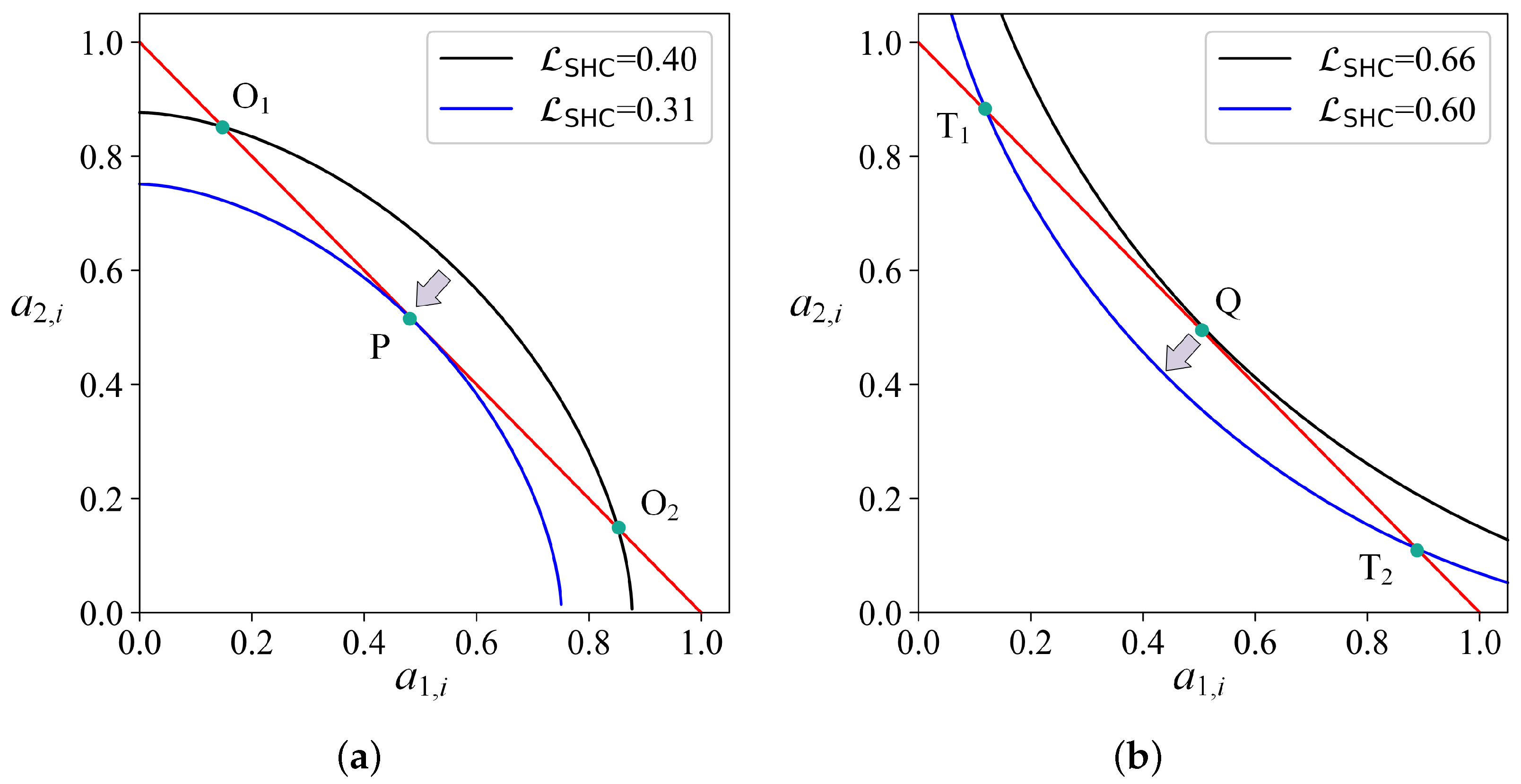
3.2. Spatial Homogeneity Constraint (${\mathcal{L}}_{\mathrm{SHC}}$)

In most of the unmixing algorithms, sparse regularization is always added to the objective function to constrain the abundance. The $l_q$ norm regularization is the commonly used term [19,43,44,56], which can be formulated as:

$${\mathcal{L}}_{\mathrm{sparse}}=\frac{1}{pn}\sum _{i=1}^p\sum _{j=1}^n{\left|a_{ij}\right|}^q$$

(12)

where q is a fixed value, which is set to 0.5 in NMF [25] and deep learning algorithms [43,44], and in semisupervised algorithms it is usually set to 2 [19]. These regularizations are based on the sparse prior and aim at reducing the number of endmembers contained in the pixels. However, not all the pixels satisfy the sparse condition. In natural scenes, mixed pixels generally exist at the junction of different materials, and the abundance of these mixed pixels should not be sparse. At these mixing regions, the spectra of pixels vary dramatically from one to another, which causes low spatial homogeneity. In contrast, the regions composed of pure pixels where the corresponding abundance vectors are more likely to be sparse tend to have a high spatial homogeneity. Noticing the distinction between mixed pixels and pure pixels in spatial homogeneity, we propose a regularization based on the spatial homogeneity constraint, denoted ${\mathcal{L}}_{\mathrm{SHC}}$:

$${\mathcal{L}}_{\mathrm{SHC}}=\frac{1}{pn}\sum _{i=1}^p\sum _{j=1}^n{\left|a_{ij}\right|}^{\mu (u,v)}$$

(13)

where $(u,v)$ is the spatial position of pixels in the image. Compared to $l_q$ norm regularization with a fixed exponent, the exponents $\mathit{\mu }$ in ${\mathcal{L}}_{\mathrm{SHC}}$ vary with the spatial homogeneity at a given spatial position $(u,v)$. ${\mathcal{L}}_{\mathrm{SHC}}$ introduces prior information about the spatial distribution of materials in a scene. As shown in Figure 1, the branch above the main encoder network is constructed to calculate the spatial homogeneity and then the spatial homogeneity map is normalized in the range of 0.5 to 2. Figure 4 demonstrates the calculation of $\mathit{\mu }$ for an HSI. A Laplacian operator is applied to the HSI to generate the spatial homogeneity map $\mathbf{M}$. Logarithmic transform is used to normalize $\mathbf{M}$. The process of normalization can be formulated as:

$$\mathit{\mu }=\mathcal{N}\left(\mathbf{M}\right)=0.5+\frac{1.5}{{log}_2(1+\gamma )}{log}_2(1+\gamma \frac{\mathbf{M}-min\left(\mathbf{M}\right)}{max\left(\mathbf{M}\right)-min\left(\mathbf{M}\right)})$$

(14)

where $\mathbf{M}$ is the spatial homogeneity map and $\gamma =50$ is the stretching factor of the logarithmic transform. For pixels with low homogeneity, the exponent of ${\mathcal{L}}_{\mathrm{SHC}}$ is close to 2 and the abundance vector tends to be average distributed. For pixels with high homogeneity, the exponent is close to 0.5 and the abundance vector tends to be sparse.

The principle of how this ${\mathcal{L}}_{\mathrm{SHC}}$ works is shown in Figure 5. In order to facilitate understanding, we demonstrate a case that contains two kinds of endmembers. The abundance of the ith pixel can be expressed as ${\mathbf{a}}_i={[a_{1,i},a_{2,i}]}^{\mathrm{T}}$, and its ${\mathcal{L}}_{\mathrm{SHC}}$ is given as:

$${\mathcal{L}}_{\mathrm{SHC}}=\frac{1}{2}\left({\left|a_{1,i}\right|}^{\mu }+{\left|a_{2,i}\right|}^{\mu }\right)$$

(15)

As shown in Figure 5, different values $\mathsf{\mu }$ and ${\mathcal{L}}_{\mathrm{SHC}}$ correspond to different curves. Meanwhile, ${\mathbf{a}}_i$ should satisfy the ASC, which means $a_{1,i}+a_{2,i}=1$ (the red line in Figure 5). The intersection points of the red line and these curves represent the abundance vectors we estimated.

The iteration process aims to minimize the value of Equation (15). When the neighborhood pixels of the ith pixel are highly mixed, the value of $\mathsf{\mu }$ is closer to 2 (i.e., $\mathsf{\mu }$ = 1.7, shown in Figure 5a). In the process of optimization, as indicated by the arrow, the curve of ${\mathcal{L}}_{\mathrm{SHC}}$ will move from the black one to the blue one, of which the value of ${\mathcal{L}}_{\mathrm{SHC}}$ is lower. In addition, the intersection point will move from point ${\mathrm{O}}_1$ or ${\mathrm{O}}_2$ to point P. The values of $a_{1,i}$ and $a_{2,i}$ tend to be close to one another, which is consistent with the high mixing characteristic of this pixel.

In contrast, if the neighborhood of the ith pixel has high homogeneity, the value of $\mathsf{\mu }$ is closer to 0.5 (i.e., $\mathsf{\mu }$ = 0.6, shown in Figure 5b). After optimization, the abundance point will move from point Q to point ${\mathrm{T}}_1$ or ${\mathrm{T}}_2$ as the curve moves down. In both cases, either $a_{1,i}$ or $a_{2,i}$ is close to 1, which is consistent with the sparse characteristic of the pure pixel.

3.3. Overall Loss Function

The total loss function ${\mathcal{L}}_{\mathrm{total}}$ in our model consists of the following three parts:

$${\mathcal{L}}_{\mathrm{total}}={\mathcal{L}}_{\mathrm{RE}}+{\lambda }_1{\mathcal{L}}_{\mathrm{SHC}}+{\lambda }_2{\mathcal{L}}_{\mathrm{scale}}$$

(16)

where ${\lambda }_1$ and ${\lambda }_2$ are the coefficients of the regularization terms, which are set to 0.05 and 0.01, respectively, in our model.

The ${\mathcal{L}}_{\mathrm{RE}}$ is the reconstruction loss function of the AE model. We use the spectral angle distance (SAD) as ${\mathcal{L}}_{\mathrm{RE}}$, which is defined as:

$${\mathcal{L}}_{\mathrm{RE}}=\frac{1}{n}\sum _{i=1}^n{cos}^{-1}\left(\frac{{{\mathbf{y}}_i}^{\mathrm{T}}{\widehat{\mathbf{y}}}_i}{∥{\mathbf{y}}_i∥∥{\widehat{\mathbf{y}}}_i∥}\right)$$

(17)

where ${\mathbf{y}}_i$ and ${\widehat{\mathbf{y}}}_i$ denote the original and reconstructed spectral of the ith pixel.

The ${\mathcal{L}}_{\mathrm{SHC}}$ and ${\mathcal{L}}_{\mathrm{scale}}$ are the regularization terms on the abundance and endmembers, respectively. ${\mathcal{L}}_{\mathrm{SHC}}$ has been discussed in detail above and will not be repeated here. The ${\mathcal{L}}_{\mathrm{scale}}$ regularization is a constraint of the scaling matrix. The aim of ${\mathcal{L}}_{\mathrm{scale}}$ is to enforce the spatial smoothness of scaling matrix S. It is defined as:

$${\mathcal{L}}_{\mathrm{scale}}=\frac{1}{np}({∥{\mathcal{H}}_h\left(\mathbf{S}\right)∥}_F^2+{∥{\mathcal{H}}_v\left(\mathbf{S}\right)∥}_F^2)$$

(18)

where ${\mathcal{H}}_h$ and ${\mathcal{H}}_v$ are linear operators of the horizontal and vertical gradients between adjacent pixels (acting separately on each endmember).

4. Experiments

In order to assess the performance of the proposed method, comparison experiments are conducted on a synthetic hyperspectral dataset as well as real datasets (Jasper Ridge dataset, Samson dataset, and Urban dataset). At first, we conduct ablation experiments to demonstrate the effectiveness of the SSA module, ELMM-based decoder, and sparse regularization term ${\mathcal{L}}_{\mathrm{SHC}}$ we proposed. Then, the proposed method is compared with the current mainstream non-deep learning unmixing algorithms [18,26] and deep learning algorithms [36,40,48] based on the LMM. It is also compared with a non-deep learning unmixing algorithm based on the ELMM [10].

In the experiment, two evaluation metrics are used to measure the accuracy of the algorithms: the mean spectral angle distance (mSAD) and average root mean square error (aRMSE), which are defined as:

$$\mathrm{mSAD}=\frac{1}{p}\sum _{j=1}^p{cos}^{-1}\left(\frac{{\mathbf{e}}_j^{\mathrm{T}}{\widehat{\mathbf{e}}}_j}{∥{\mathbf{e}}_j∥∥{\widehat{\mathbf{e}}}_j∥}\right)$$

(19)

$$\mathrm{aRMSE}=\sqrt{\frac{{\sum }_{i=1}^n{∥{\mathbf{a}}_i-{\widehat{\mathbf{a}}}_i∥}^2}{pn}}$$

(20)

where ${\mathbf{e}}_j$ and ${\widehat{\mathbf{e}}}_j$ are the real spectrum and the extracted spectrum of the jth endmember, respectively, and ${\mathbf{a}}_i$ and ${\widehat{\mathbf{a}}}_i$ denote the ground truth of abundance and the estimated abundance, respectively, of the ith pixel.

The proposed network is implemented under the TensorFlow framework. The learning rate is initialized with 0.001, and an exponential decay schedule is applied to adjust the learning rate during training (decay steps = 10, decay rate = 0.9). The network runs for 500 epochs. The endmember matrix is initialized with the endmembers extracted in Section 4.2. The scaling factor matrix is initialized to 1. In the first 100 epochs, the endmember matrix and scaling factor matrix are fixed to generate a good initialization of the encoder.

4.1. Data Description

(1) Synthetic dataset

Figure 6a shows a color image of the synthetic dataset. The synthetic dataset is generated as follows: First, 5 endmembers are randomly selected from the United States Geological Survey (USGS) spectral library. White Gaussian noise is added to these endmembers. The standard deviation of the white Gaussian noise is 0.1. Then, the abundance distribution of each endmember is randomly generated and combined through the extended linear mixing model. The scaling factors are limited between 0.8 and 1.2 and uniformly distributed. Finally, a 20 dB white Gaussian noise is added to these pixels. This synthetic dataset is of 120 × 120 pixels and contains 5 endmembers with 431 bands. The 5 endmembers selected from USGS are asphalt, PVC, sheetmetal, brick, and fiberglass.

(2) Real dataset

The real datasets are downloaded from the Remote Sensing Laboratory website (https://rslab.ut.ac.ir/data, accessed on 5 March 2021). The commonly used datasets for hyperspectral unmixing are the Jasper Ridge, Samson, and Urban datasets, which are shown in Figure 6b–d, respectively.

The Samson dataset contains 95 × 95 pixels. Each pixel is observed at 156 bands covering the spectra from 401 nm to 889 nm, which has little water vapor impact and no serious noise. The Samson dataset has three types of endmembers: water, tree, and soil.

The Jasper Ridge dataset contains 100 × 100 pixels. Each pixel records 224 bands ranging from 380 nm to 2500 nm. Due to the influence of water vapor absorption, bands 1–3, 108–112, 154–166, and 220–224 are not available, so only the remaining 198 bands are retained for experiments. The Jasper Ridge dataset includes four types of endmembers: water, tree, soil, and road.

The Urban dataset is a more complex unmixing dataset. There are 307 × 307 pixels in this image. The image has 210 spectral bands covering the wavelengths from 400 nm to 2500 nm. After removing the badly degraded bands 1–4, 76, 87, 101–111, 136–153, and 198–210 caused by water vapor and atmospheric effects, there remain 162 bands for the experiments. This dataset contains both artificial and natural objects, which are tree, grass, roof, asphalt, metal, and soil.

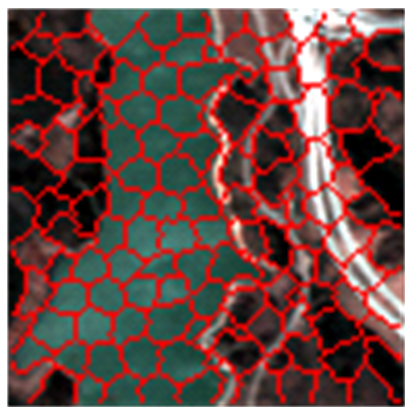
4.2. Endmember Initialization

Endmember initialization is the precursor work of the unmixing algorithm. The accuracy of the extracted endmembers greatly impacts the unmixing results. Most endmember-extraction algorithms are based on the geometric properties of endmembers in the spectral space. However, these methods are seriously affected by noise and outliers. Therefore, we use a more stable method that combines simple linear iterative clustering (SLIC) [57] and VCA to initialize the endmember matrix. The SLIC operation on the space and spectrum can generate a super-pixel segmentation on the hyperspectral data. An example of SLIC on the Jasper Ridge dataset is shown in Figure 7. After obtaining the super-pixels, the cluster centers of each super-pixel can be regarded as approximate pure pixels. These cluster centers are less sensitive to noise and outliers because they are the regional average of similar pixels. Using the spectra of these center pixels as candidates to extract endmembers would be more reliable. Then, we choose VCA as the following operation to extract the initial endmembers.

The ATGP [58], Nfindr [13], VCA [12], and SGSNMF [26] algorithms are selected as the comparison algorithms for endmember extraction.

Table 1. mSAD (rad) results of SLIC-VCA on each dataset.

	SLIC-VCA	VCA	Nfindr	ATGP	SGSNMF
Synthetic	0.0463	0.0285	0.1332	0.1469	0.0363
Samson	0.0530	0.0756	0.0583	0.4185	0.0921
Jasper Ridge	0.0764	0.1538	0.1376	0.4949	0.1726
Urban	0.1001	0.5194	0.3566	0.3790	0.4028

shows the results of the extracted endmembers on all datasets. According to the SAD results, the SLIC-VCA algorithm achieves the best results on real datasets. Especially on the Urban dataset, the extracted endmembers are much better than other methods, which indicates that the SLIC-VCA method adapts to complex natural scenes well. For the synthetic dataset, the SLIC-VCA algorithm yields the third-best value of mSAD. However, Figure 8 shows that the result of the SLIC-VCA algorithm on the synthetic dataset obtains a closer absolute value compared to VCA and SGSNMF. This means that SLIC-VCA is less affected by the endmember scaling factors added in the synthetic dataset. These results confirm the effectiveness of the endmember-initialization method.

4.3. Ablation Experiments

Ablation experiments are conducted on the Samson dataset and Jasper Ridge dataset to verify the effectiveness of our proposed method. The ablation experiments consist of three parts, which are related to the three highlights of the proposed method, respectively.

4.3.1. The Effect of SSA Module

In order to analyze the effectiveness of the proposed SSA module, four conditions are set in this ablation experiment. The first one is removing the SSA module, the second one is only using the non-local attention module, the third one is only using the spectral attention module, and the fourth one is using the proposed SSA module.

Table 2. RMSE results of ablation experiments on the SSA module.

Datasets	Non-Local Attention Module	Spectral Attention Module	Water	Tree	Soil	Road	aRMSE
Samson	✘	✘	0.1166	0.0798	0.1216	-	0.1077
	✔	✘	0.0966	0.0747	0.1056	-	0.0932
	✘	✔	0.0924	0.1000	0.1056	-	0.0995
	✔	✔	0.0626	0.0798	0.0996	-	0.0825
Jasper Ridge	✘	✘	0.0523	0.0984	0.1228	0.1158	0.1012
	✔	✘	0.0617	0.0822	0.1328	0.1038	0.0987
	✘	✔	0.0511	0.0746	0.1228	0.1038	0.0923
	✔	✔	0.0523	0.0724	0.1108	0.0878	0.0838

shows the abundance-estimation results of each condition. The aRMSE results of cases without the SSA module are the worst. After adding either the non-local attention module or the spectral attention module, the unmixing performance improves to a certain degree. The best results are achieved by using the SSA module. These results demonstrate the effectiveness of the SSA module and its two branches.

In order to analyze the computational complexity caused by using SSA, the computational time of the aforementioned four conditions on the four datasets are summarized in

Table 3. The processing time of ablation experiments on the SSA module (s).

Non-Local Attention Module	Spectral Attention Module	Synthetic	Samson	Jasper Ridge	Urban
✘	✘	37.18	24.06	27.05	88.36
✔	✘	92.50	37.76	40.35	484.65
✘	✔	54.61	39.77	47.70	108.37
✔	✔	107.88	53.75	58.42	532.74

. The algorithm is implemented in Python (3.8) and TensorFlow (2.7.0). The network is run on a computer with an Intel Xeon E5-2620 v4 processor, 48 GB of memory, a 64-bit operating system, and an NVIDIA GeForce GTX (1080 Ti) graphical processing unit. It is evident across all datasets that the non-local attention module increases the computing time more than the spectral attention module does. Additionally, the SSA module, which combines the two modules, takes the longest time to complete. Furthermore, with the Urban dataset, the computing time dramatically increases. This might be because this dataset has more pixels and more intricate geographical information than the other datasets, which could increase the computational complexity.

4.3.2. The Effect of Scaling Matrix

To analyze the impact of the ELMM introduced in our decoder, we compare the unmixing results with/without the scaling matrix.

Table 4. RMSE comparison of different scaling factor matrix settings.

Datasets		Water	Tree	Soil	Road	aRMSE
Samson	with $\mathbf{S}$	0.0626	0.0798	0.0996	-	0.0825
	without $\mathbf{S}$	0.0955	0.0633	0.1117	-	0.0924
Jasper Ridge	with $\mathbf{S}$	0.0523	0.0724	0.1108	0.0878	0.0838
	without $\mathbf{S}$	0.0567	0.0827	0.1138	0.0988	0.0906

shows the results under different settings. The aRMSEs of both datasets are both smaller with the scaling factor matrix $\mathbf{S}$ than those without $\mathbf{S}$. This ablation experiment demonstrates that the introduction of the ELMM in our decoder can improve the unmixing performance of the network.

4.3.3. The Effect of ${\mathcal{L}}_{\mathrm{SHC}}$

To verify the effectiveness of our proposed spatial homogeneity constraint ${\mathcal{L}}_{\mathrm{SHC}}$ on the abundance, we compare the ${\mathcal{L}}_{\mathrm{SHC}}$ with the commonly used ${\mathcal{L}}_{1/2}$ loss ($\mathsf{\mu }$ is fixed at 0.5) and ${\mathcal{L}}_2$ loss ($\mathsf{\mu }$ is fixed at 2). The unmixing results are summarized in

Table 5. RMSE comparison of different loss functions.

Datasets		Water	Tree	Soil	Road	aRMSE
Samson	${\mathcal{L}}_{\mathrm{SHC}}$ loss	0.0626	0.0798	0.0996	-	0.0825
	${\mathcal{L}}_{1/2}$ loss	0.0958	0.0637	0.1107	-	0.0922
	${\mathcal{L}}_2$ loss	0.0982	0.0705	0.1087	-	0.0939
Jasper Ridge	${\mathcal{L}}_{\mathrm{SHC}}$ loss	0.0523	0.0724	0.1108	0.0878	0.0838
	${\mathcal{L}}_{1/2}$ loss	0.0557	0.0775	0.1139	0.0962	0.0886
	${\mathcal{L}}_2$ loss	0.0515	0.0809	0.1185	0.1054	0.0927

. The proposed ${\mathcal{L}}_{\mathrm{SHC}}$ generates the best results of aRMSE, followed by the ${\mathcal{L}}_{1/2}$ loss, and ${\mathcal{L}}_2$ loss yields the worst results. The impact of the ${\mathcal{L}}_{\mathrm{SHC}}$ constraint can also be seen in the comparison in Figure 9. As the value of $\mathsf{\mu }$ becomes higher, the abundance maps become more uniformly distributed, which is consistent with our analysis in Section 3.2.

4.4. Comparison Experiments

In this section, comparison experiments are carried out between our proposed method and other deep learning methods as well as traditional methods. The compared methods are as follows:

(1)

FCLSU [18]: The most-widely used method of abundance estimation. It should be coupled with an endmember-extraction method. In our experiments, the endmember is also extracted using the SLIC-VCA initial method.

(2)

SGSNMF [26]: An NMF method cooperating with spatial group sparsity regularization. The abundances and endmembers are initialized by the results of FCLSU.

(3)

DAEU [38]: A deep-learning-based method for blind hyperspectral unmixing using an autoencoder structure. This network uses fully connected layers to extract the features of the pixel-wise spectra input.

(4)

CNNAEU [40]: A CNN-based unmixing autoencoder network using patches of HSIs as input to exploit the spatial information of the image.

(5)

PGMSU [48]: A unmixing autoencoder considering spectral variability through a variational autoencoder (VAE). This method uses VAE to generate different endmembers for each pixel.

(6)

ELMM [10]: A linear unmixing model considering spectral variability introduced in Section 2.2, which is also the model of the decoder used in our method. It uses the alternating non-negative least squares (ANLS) to solve the problem. It is also worth noting that spatial similarity regularization is implemented in the object function.

On each dataset, the SGSNMF, DAEU, CNNAEU, PGMSU, and proposed MAAENet experiments are run ten times independently. The mean value and standard deviation of RMSE are calculated and summarized in the following experiments.

4.4.1. Synthetic Dataset

Table 6. RMSE of the synthetic dataset.

	MAAENet	FCLSU	SGSNMF	DAEU	CNNAEU	PGMSU	ELMM
Asphalt	0.0742 ± 0.0052	0.0872	0.1266 ± 0.0035	0.1234 ± 0.0254	0.2456 ± 0.1218	0.0982 ± 0.0206	0.1051
PVC	0.0569 ± 0.0059	0.0742	0.0781 ± 0.0011	0.2004 ± 0.0483	0.1826 ± 0.0760	0.1258 ± 0.0176	0.1402
Sheetmetal	0.0574 ± 0.0039	0.0534	0.0623 ± 0.0002	0.1212 ± 0.0424	0.1538 ± 0.0548	0.0721 ± 0.0221	0.0975
Brick	0.0727 ± 0.0029	0.0774	0.0626 ± 0.0014	0.2188 ± 0.0225	0.2785 ± 0.056	0.1136 ± 0.0140	0.1322
Fiberglass	0.0701 ± 0.0020	0.0713	0.0536 ± 0.0003	0.1205 ± 0.0371	0.2001 ± 0.0984	0.0774 ± 0.0124	0.0833
aRMSE	0.0668 ± 0.0011	0.0735	0.0810 ± 0.0010	0.1655 ± 0.0136	0.2458 ± 0.0228	0.1003 ± 0.0113	0.1137

and Figure 10 demonstrate the RMSE results and abundance maps of the synthetic dataset obtained using different methods. Our technique has a lower aRMSE than the competing methods. Moreover, it is clear from the abundance maps that noise has a significant impact on FCLSU. Because of the random initialization of endmembers, DAEU and CNNAEU produce inferior results, which suggests that a reliable initialization of endmember is required. The PGMSU abundance maps are overly smoothed, while the ELMM abundance maps are very sharp.

We add Gaussian noises of 10 dB, 20 dB, and 30 dB to the synthetic dataset in order to show how the suggested technique performs under various noise levels. As indicated in Table 6, FCLSU is the second-best method overall. Hence, it is selected to process the synthetic datasets with noise for comparison. The RMSE results of the synthetic dataset with noise are displayed in

Table 7. RMSE of the synthetic dataset under different noise levels.

	10 dB		20 dB		30 dB
	MAAENet	FCLSU	MAAENet	FCLSU	MAAENet	FCLSU
Asphalt	0.0763 ± 0.0025	0.0917	0.0742 ± 0.0052	0.0872	0.0691 ± 0.0056	0.0844
PVC	0.0691 ± 0.0036	0.1137	0.0569 ± 0.0059	0.0742	0.0539 ± 0.0038	0.0588
Sheetmetal	0.0599 ± 0.0028	0.0653	0.0574 ± 0.0039	0.0534	0.0541 ± 0.0014	0.0454
Brick	0.0824 ± 0.0032	0.1010	0.0727 ± 0.0029	0.0774	0.0723 ± 0.0020	0.0724
Fiberglass	0.0748 ± 0.0015	0.0755	0.0701 ± 0.0020	0.0713	0.0632 ± 0.0041	0.0600
aRMSE	0.0729 ± 0.0011	0.0911	0.0668 ± 0.0011	0.0735	0.0630 ± 0.0012	0.0656

shows. As can be observed, our method MAAENet performs better at all three noise levels compared with FCLSU. Additionally, unlike FCLSU, the unmixing results of MAAENet do not significantly degrade when the noise level rises. This implies that the proposed MAAENet has a lower sensitivity to noise than FCLSU.

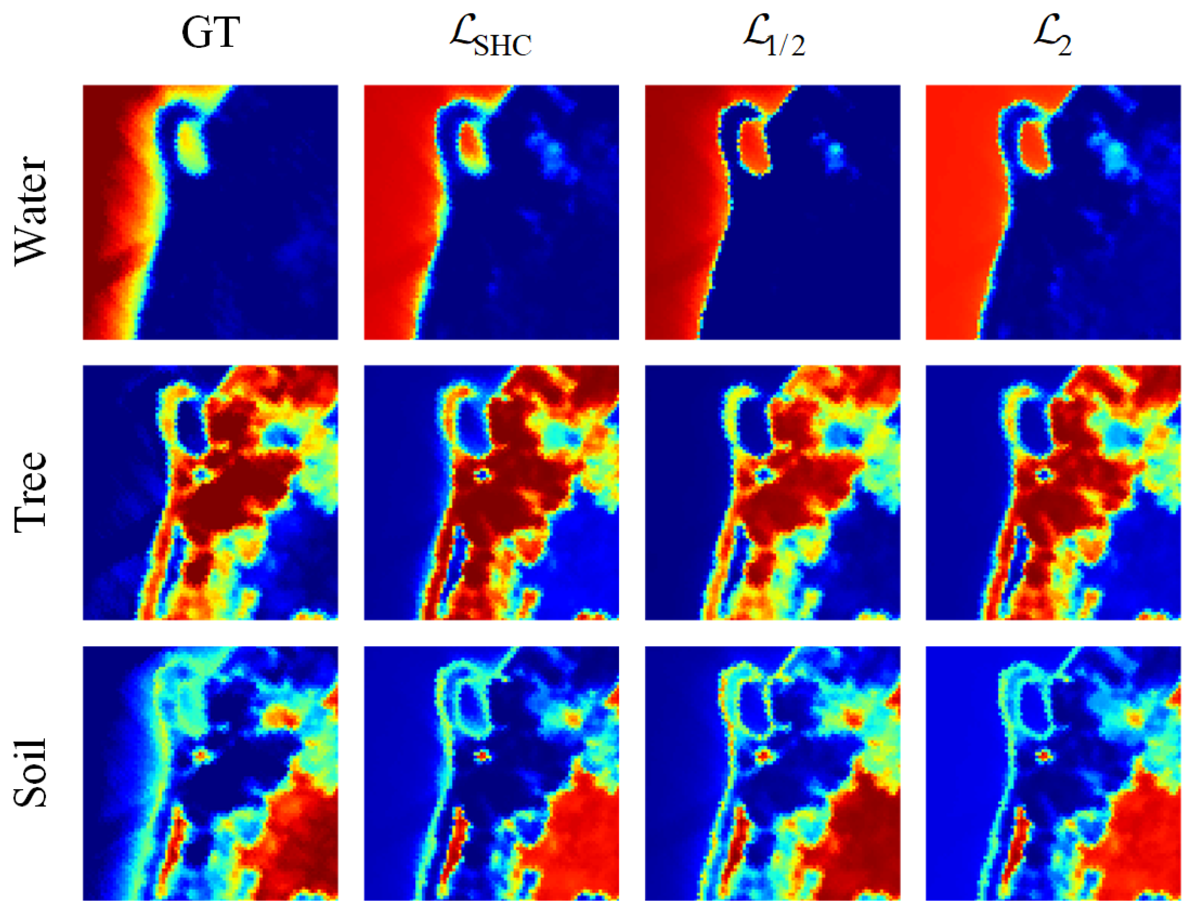
4.4.2. Samson Dataset

The abundance RMSE results of all the methods on the Samson dataset are shown in

Table 8. RMSE of the Samson dataset.

	MAAENet	FCLSU	SGSNMF	DAEU	CNNAEU	PGMSU	ELMM
Water	0.0626 ± 0.0183	0.2720	0.3884 ± 0.0005	0.0515 ± 0.0174	0.2164 ± 0.0285	0.2898 ± 0.0140	0.2340
Tree	0.0798 ± 0.0059	0.1507	0.2699 ± 0.0003	0.1367 ± 0.0696	0.2144 ± 0.0480	0.1647 ± 0.0113	0.1367
Soil	0.0996 ± 0.0086	0.1817	0.1928 ± 0.0005	0.1050 ± 0.0207	0.1663 ± 0.0551	0.3153 ± 0.0191	0.1603
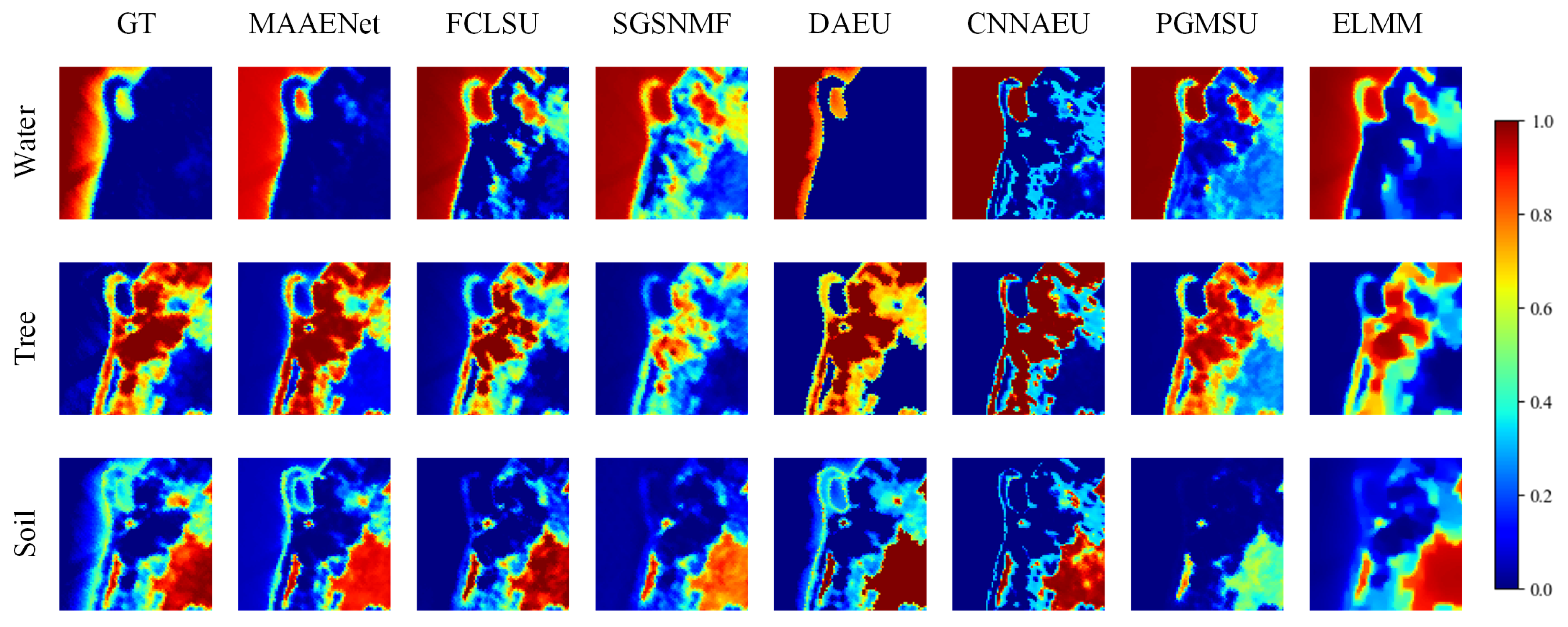
aRMSE	0.0825 ± 0.0075	0.2079	0.2947 ± 0.0004	0.1069 ± 0.0327	0.2035 ± 0.0215	0.2650 ± 0.0137	0.1818

. It can be seen that our approach outperforms deep learning, geometrical, and NMF-based approaches. The outcomes of traditional unmixing techniques such as FCLSU and SGSNMF are inferior. Since spectral variability is considered in the method, the results of the ELMM algorithm are improved slightly. However, as we can see from Figure 11, the ELMM algorithm’s adoption of a smoothing requirement results in the abundance maps being overly smoothed. The findings obtained with the DAEU are second-best. The CNNAEU abundance results have a propensity to be 1, meaning that an abundance map is roughly equivalent to a classification map. Moreover, Figure 11 demonstrates how significantly different the abundance map of the soil material produced using PGMSU is from the ground truth.

4.4.3. Jasper Ridge Dataset

Table 9. RMSE of the Jasper Ridge dataset.

	MAAENet	FCLSU	SGSNMF	DAEU	CNNAEU	PGMSU	ELMM
Water	0.0523 ± 0.0037	0.1270	0.1780 ± 0.0028	0.1375 ± 0.0232	0.2291 ± 0.0969	0.1193 ± 0.0038	0.1090
Tree	0.0724 ± 0.0062	0.1062	0.1460 ± 0.0119	0.0788 ± 0.0084	0.2459 ± 0.0076	0.0970 ± 0.0045	0.0734
Soil	0.1108 ± 0.0088	0.1755	0.1794 ± 0.0566	0.1456 ± 0.0278	0.3466 ± 0.0244	0.0807 ± 0.0026	0.1726
Road	0.0878 ± 0.0115	0.1832	0.1272 ± 0.0121	0.2237 ± 0.0223	0.3215 ± 0.0911	0.0624 ± 0.0022	0.1392
aRMSE	0.0838 ± 0.0063	0.1515	0.1609 ± 0.0139	0.1558 ± 0.0146	0.2943 ± 0.0382	0.0923 ± 0.0015	0.1289

demonstrates how our technique regularly outperforms the competition when used on the Jasper Ridge dataset. Figure 12 provides an illustration of the abundance maps. With more endmembers in the scene, the performance of the other two deep learning techniques, CNNAEU and DAEU, drops off considerably. The random initialization spectra of endmembers could be the main reason for CNNAEU’s inaccuracy. The second-best results are obtained with PGMSU, and the third-best results are attained with ELMM. This suggests that the Jasper Ridge dataset’s endmember spectra contain significant spectral variability. Thus, in this situation, spectral-variability-based approaches are preferable.

4.4.4. Urban Dataset

Table 10. RMSE of the Urban dataset.

	MAAENet	FCLSU	SGSNMF	DAEU	CNNAEU	PGMSU	ELMM
Tree	0.1092 ± 0.0101	0.2373	0.2364 ± 0.0041	0.1766 ± 0.0857	0.2074 ± 0.0152	0.1515 ± 0.0119	0.4499
Grass	0.1292 ± 0.0061	0.2037	0.1662 ± 0.0417	0.2347 ± 0.0163	0.2831 ± 0.0228	0.1954 ± 0.0165	0.1880
Roof	0.0834 ± 0.0092	0.1461	0.1787 ± 0.0062	0.1861 ± 0.0830	0.1936 ± 0.0721	0.1145 ± 0.0052	0.4343
Asphalt	0.1465 ± 0.0069	0.3083	0.3466 ± 0.0565	0.1591 ± 0.0233	0.2993 ± 0.0744	0.1735 ± 0.0054	0.4304
Metal	0.0993 ± 0.0347	0.1312	0.1196 ± 0.0297	0.1916 ± 0.0096	0.1511 ± 0.0314	0.1154 ± 0.0013	0.0875
Soil	0.1023 ± 0.0175	0.1805	0.1480 ± 0.0057	0.2262 ± 0.0280	0.2155 ± 0.0268	0.1471 ± 0.0062	0.1501
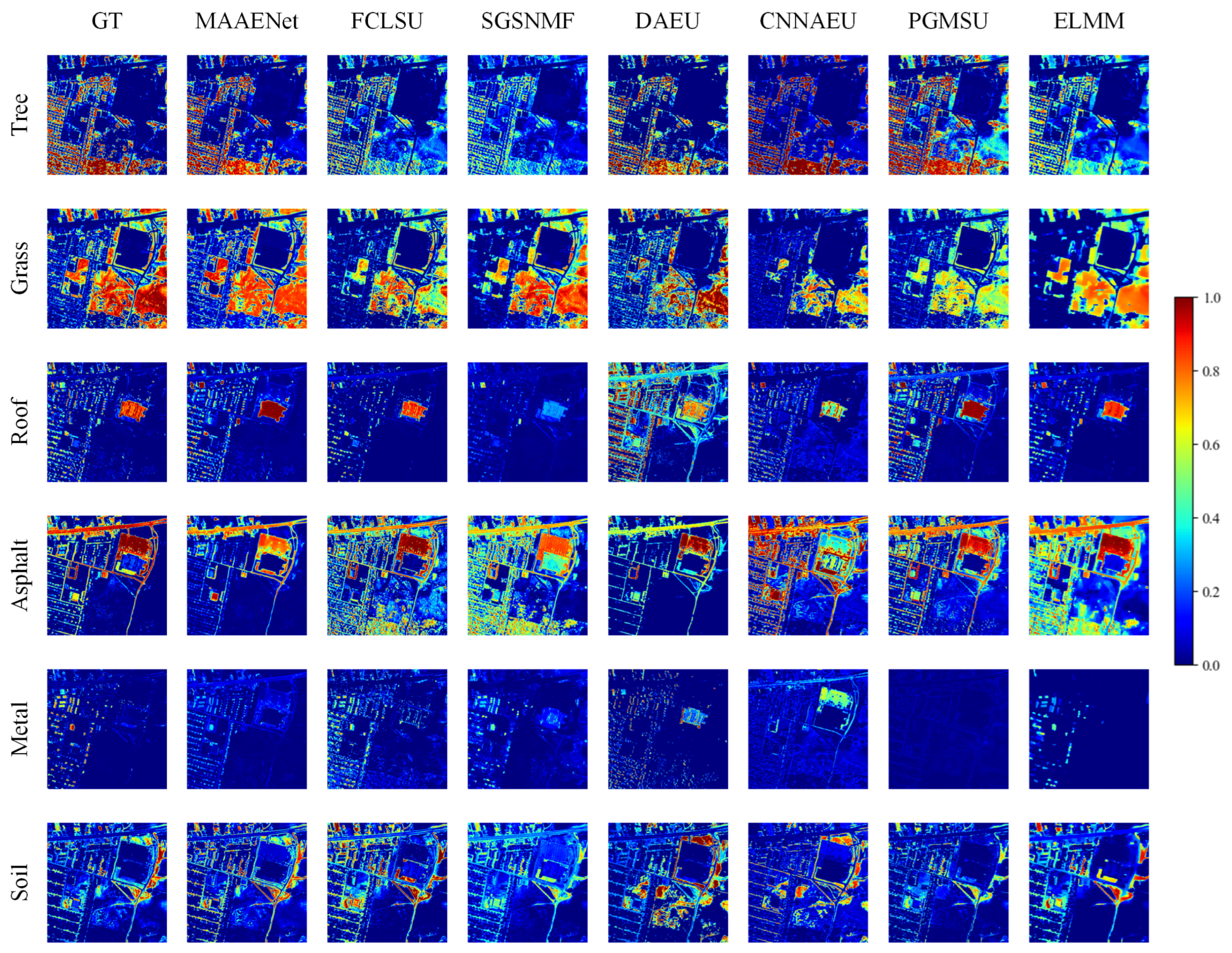
aRMSE	0.1196 ± 0.0083	0.2090	0.2173 ± 0.0219	0.2028 ± 0.0080	0.2334 ± 0.0259	0.1525 ± 0.0052	0.3271

and Figure 13 show the unmixing results on the Urban dataset. This dataset contains a complicated scene with six different materials. Even so, our approach continues to perform better than the other competing methods. On both the tree and the asphalt material, the FCLSU, SGSNMF, and ELMM abundance maps are significantly worse. Moreover, ELMM also performs more poorly on the roof material. DAEU, CNNAEU, and PGMSU, which are deep-learning-based algorithms, perform worse on the metal material.

5. Conclusions

An ELMM-based deep learning system called MAAENet was introduced in this study to address endmember variability. In the decoder, scaling factors were added to model the spectral variability. An SSA module based on attention mechanisms was designed in the encoder to gather the global spatial information and reweight each band of HSIs. To further limit the sparsity of abundance and collect local spatial features, a flexible regularization based on geographic homogeneity was included in the total loss function. The endmember matrix was initialized using VCA from the cluster centers of SLIC results. Experiments were conducted on a synthetic dataset and three real datasets. The benefits of the SLIC-VCA approach were demonstrated by the endmember extraction findings. The ablation experiments demonstrated the usefulness of the specially designed decoder, SSA module, and ${\mathcal{L}}_{\mathrm{SHC}}$. Furthermore, compared to existing unmixing approaches, our method could produce better results for abundance estimation in all datasets. Additionally, the experimental findings demonstrated that even as the number of endmembers increased, our technique could still deliver a competitive performance. Future studies could explore the spectral variability of endmember further by adding prior knowledge and using more complex nonlinear mixing models. In addition, recently, graph convolution networks (GCN) have been proposed for classification using hyperspectral images [59]. We could build autoencoder networks using the GNN architecture to achieve better representation and improve the unmixing performance.