Article

Multi-Node Motion Estimation Method Based on B-Spline of Array Position and Orientation System

School of Instrumentation Science and Optoelectronic Engineering, Beijing University of Aeronautics and Astronautics, Beijing 100191, China
*
Author to whom correspondence should be addressed.
Remote Sens. 2023, 15(11), 2892; https://doi.org/10.3390/rs15112892
Submission received: 25 April 2023 / Revised: 26 May 2023 / Accepted: 29 May 2023 / Published: 1 June 2023

Abstract

:
The array position and orientation system (array POS), composed of one main POS and multiple sub-inertial measurement units (sub-IMUs), is key equipment in the aerial remote-sensing system, especially the multi-load system, which can provide motion compensation for the multi-load remote-sensing system to improve imaging quality. Nevertheless, the measurement information of each sub-IMU can only realize the motion information of the corresponding remote-sensing load. Ideally, each remote-sensing load should be equipped with a sub-IMU for motion compensation, which is impossible in actual engineering considering the volume, weight and cost. To solve this problem, a multi-node motion estimation method based on the B-spline of the array POS is proposed to realize the motion compensation of remote-sensing loads without sub-IMUs. Firstly, the transfer alignment method based on fiber-grating multi-dimensional deformation measurement was adopted. Motion parameters of the remote-sensing payload equipped with sub-IMUs at different times can be obtained by observing and correcting the errors between the main POS and sub-IMUs. In this way, the space-time characteristics of each interpolation point are fully utilized. Additionally, the motion information of the main POS and all sub-IMUs is fitted through the estimation method based on the B-spline, during which wing deformation is considered to obtain the motion parameters of the remote-sensing payload equipped without a sub-IMU. In this way, the spatial correlation between the information of each node is fully utilized. Due to the full utilization of the spatiotemporal correlation of the motion information of each sub node, high-precision and highly reliable motion information of the remote-sensing loads not equipped with sub-IMUs is obtained. Furthermore, the proposed method can be modified locally without affecting other nodes, and has the advantages of a simple algorithm and easy engineering implementation. Finally, a semi-physical simulation based on ground-loading test was conducted. The results show that the baseline in the X-axis, Y-axis and Z-axis direction is improved by 0.484 mm, 0.137 mm and 1.225 mm, respectively, and that the measurement accuracy of roll angle is improved by 0.011°.

Graphical Abstract

1. Introduction

The aerial earth observation platform with multiple tasks and functions is the frontier development direction of aerial remote-sensing technology, and the attitude and position precision of the aerial earth observation platform is critical to the precision of multiple measuring instruments such as the aerial cameras, imaging spectrometers, scanning laser and synthetic aperture radar installed on it [1,2,3,4]. Especially, the measuring instruments are installed on different positions of the airplane, so the several inertial measurement units (IMUs) should be equipped with measuring instruments to accurately obtain attitude and position information with transfer alignment at multiple nodes [5,6,7,8]. Therefore, the array position and orientation measurement system (array POS) technology with array sub-IMUs and the main POS unit are critical to obtain the attitude and position information of measurement instruments [9,10,11]. Usually, the main POS unit is installed on the belly, and the array sub-IMUs are installed as close as possible to the imaging loads on the wing to complete motion compensation. It is known that the motion error of the remote-sensing loads installed with the sub-IMU can be directly measured and compensated, while the motion error of the remote-sensing loads without sub-IMU cannot be directly measured and compensated [12,13,14,15]. From the perspective of system engineering implementation, it is obviously unreasonable to install sub-IMUs on each remote-sensing load considering the volume, weight and cost. How to use the motion information of the remote-sensing loads installed with the sub-IMUs to obtain the motion information of the remote-sensing load without sub-IMUs is an urgent problem to be solved, which can be attributed to a fitting problem [16,17,18]. Interpolation and approximation are two commonly used methods to solve this problem [19,20]. The common point of the two methods is to use a set of discrete points to obtain the equations describing these discrete points. The interpolation method requires that all the equations pass through these known discrete points, while the approximation method only requires being as close as possible to these known discrete points under the condition that certain rules are met. The commonly used approximation method is the least squares fitting method, which searches for the best-fitting curve to a given set of points by minimizing the sum of squares of errors [21,22]. The moment of all remote-sensing loads installed on the wing is related, since the deformation of an aircraft wing caused by gust and turbulence during flight is continuous, which is not taken into account in the fitting process of the lowest quadratic fitting method. As a result, the fitting accuracy of the least square method is relatively low. As a special form of expression for spline curves, the B-spline is a linear combination of B-spline basis functions which achieves better control over the curve by decoupling the control points and order. Additionally, B-splines handle the smoothness constraints in a very elegant fashion and provide a basis with excellent numerical properties. That is, the B-spline fusion with strong flexibility can locally control and smooth the profile of curves, thus it is a common interpolation method for aerodynamic shape curve and surface [23,24,25]. All the characteristics of the B-spline mentioned above are applicable to the motion information fitting based on wing deformation in this paper. The results of the semi-physical simulation based on ground-loading testing reflect the superiority of the B-spline fusion interpolation method.
This article is organized as follows. In Section 2, the array POS and the mathematical model are briefly introduced at first. Then the global estimation model based on the B-spline fusion interpolation method is developed to obtain the motion parameters of a remote-sensing payload without sub-IMU. In Section 3, the semi-physical simulation is carried out, and the experimental setup, processing and results are elaborated in detail, which verifies the correctness of the proposed method. The conclusion and discussion are given in Section 4.

2. Materials and Methods

2.1. Composition of the Array POS

The array POS is illustrated in Figure 1, which includes the main POS, multiple IMU devices, the deformation-sensing unit, the information-processing unit and the information processing software. As shown in Figure 1, the main POS consists of the main IMU and the GNSS receiver, and the main IMU is installed on the airplane cabin to work together with the GNSS receiver, and then the high-precision motion parameters of the master node are obtained. The sub-IMU devices are installed on the different nodes of the airplane wing, and high-precision measurement of the sub-inertial navigation system is realized by the transfer alignment between the main POS and the sub-IMU devices, and the transfer alignment model is described in detail as below. However, the relative motion between the main POS and the sub-IMUs caused by the flexible deformation of the airplane wing could reduce the precision of the transfer alignment between them during high-speed motion. Thus, the deformation-sensing unit with fiber-grating sensors is added in the array POS, which can easily measure the flexible deformation. The information processing unit based on the FPGA + DSP board could receive and process in a timely manner the data of the main POS, multiple IMU devices and the deformation-sensing unit. Moreover, the collected data can be combined and filtered with information-processing software, including real-time processing software and post-processing software.

2.2. Design of Transfer Alignment for the Array POS

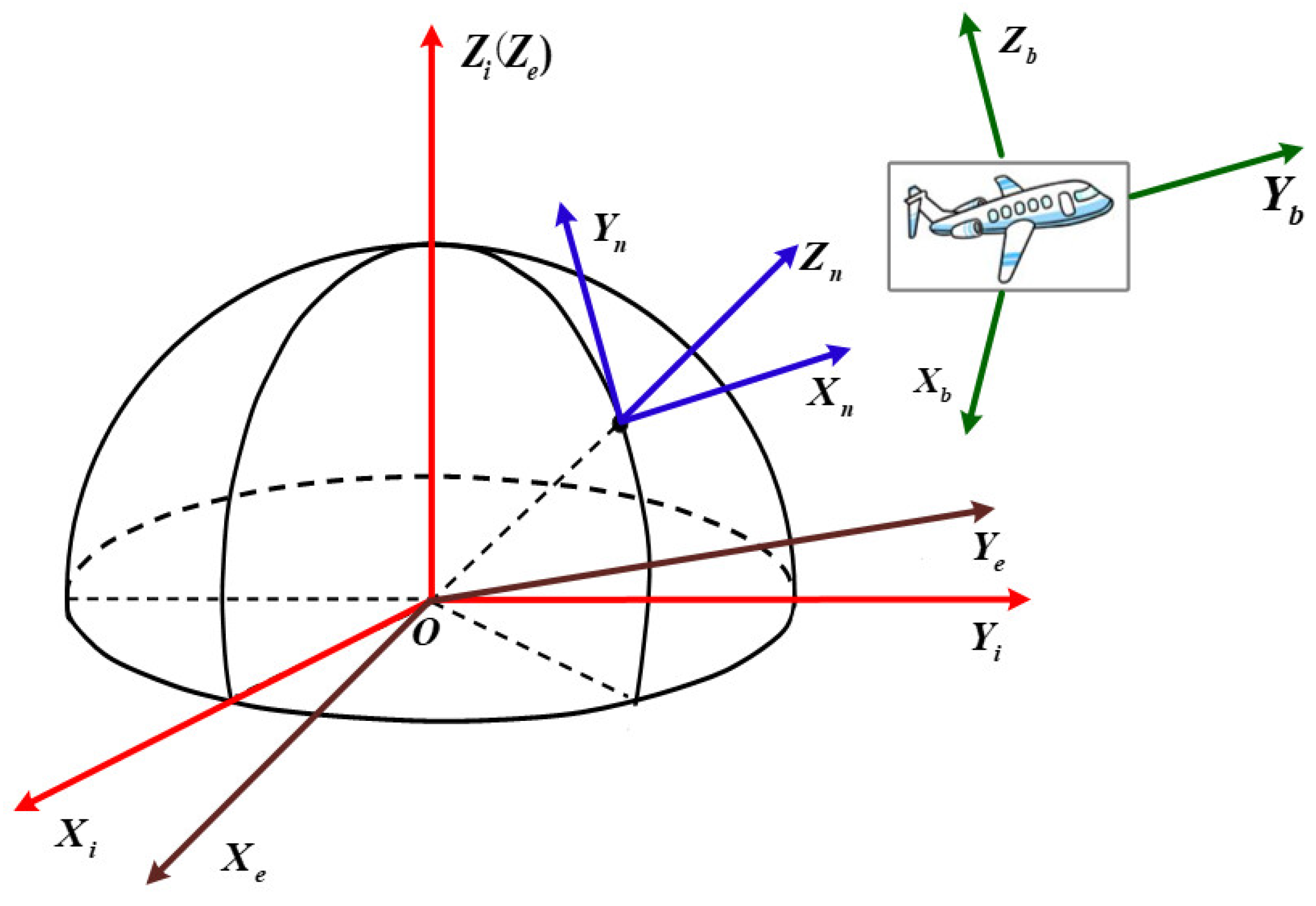
As is mentioned above, the motion parameters of the sub-IMU are mainly obtained by transfer alignment. The transfer alignment of the array POS is presented in detail in this section. There are some reference coordinate frames used in model building, which includes the inertial frame (i-frame) indicated by the solid red line, the earth frame (e-frame) indicated by the solid brown line, the navigation frame (n-frame) indicated by the solid blue line and the body frame (b-frame) indicated by the solid green line in Figure 2. It is noted that the geography frame is taken as the navigation frame.
In this section, the mathematical model for the transfer alignment is established. The output value of the high-precision master POS is identified as the reference in the transfer alignment, which finally realizes the compensation of the sub-IMU output information and improves its accuracy by using the optimal estimation of sub-IMU error parameters with appropriate filtering algorithm. The state equation and observation equation of the transfer alignment are shown as follows.

2.2.1. State Equation

The mathematical model of the transfer alignment is established on the basis of the inertial navigation system error equation [16], which is not repeated here. The state equation of the transfer alignment can be shown as Equation (1).
X ˙ ( t ) = F ( t ) X t + G ( t ) w ( t )
where X ( t ) is the state variable of 15 dimensions, the expression of which is shown as Equation (2). F ( t ) is the state transition matrix [16], which is not repeated here. G ( t ) is the system noise matrix as shown in Equation (3). Through w ( t ) marks the system noise-driving matrix, as shown in Equation (4).
X ( t ) = [ ϕ x , ϕ y , ϕ z , δ V x , δ V y , δ V z , δ L , δ λ , δ H , ε x , ε y , ε z , x , y , z ] T
ϕ x , ϕ y and ϕ z are the relative misalignment angles in X axis, Y axis and Z axis direction between the main POS and the sub-IMU in two navigation coordinate frames. δ V x , δ V y and δ V z are, respectively, the velocity errors in the X axis, Y axis and Z axis direction between the main POS and the sub-IMU in two navigation coordinate frames. δ L , δ λ , δ H are, respectively, the latitude error, longitude error and the height error between the main POS and the sub-IMU. ε x , ε y and ε z are the random constant drift of gyroscopes, respectively, in the x-axis, y-axis and z-axis direction. x , y and z are the constant offsets of the accelerometer, respectively, in the x-axis, y-axis and z-axis direction.
G ( t ) = C b n 0 3 3 0 3 3 C b n 0 9 3 0 9 3
w ( t ) = w ε x w ε y w ε z w x w y w z w φ w γ w γ x w γ y T
where w ε x , w ε y and w ε z are the random error of the gyroscope in the x-axis, y-axis and z-axis direction, respectively, and w x , w y and w z are the random error of the accelerometer in the x-axis, y-axis and z-axis direction, respectively. w φ is the misalignment angle error. w γ is the lever arm error between main POS and the sub-IMU. w γ x and w γ y are the lever arm error between main POS and the sub-IMU in the x-axis and y-axis, respectively.

2.2.2. Observation Equation

  • Observation equation of main POS:
The transfer alignment method based on fiber-grating measurement for the array POS is adopted in this paper, where the measured information is compensated by the three-dimensional position and attitude information provided by the fiber grating. The “position and attitude” matching pattern is selected in this paper, and the observation equation is shown as Equation (5).
Z = H X + v
where Z is the observation and can be expressed as Equation (6). The measurement noise is denoted by v , which can be regarded as Gaussian white noise with zero mean value. The expression of the measurement noise is shown in Equation (7). H is the measurement matrix, which is shown as Equation (8).
Z = δ L δ λ δ h δ ψ δ θ δ γ T = Z p Z a T
where δ L , δ λ and δ H are, respectively, the latitude error, longitude error and the height error between the main POS and the sub-IMU. δ φ , δ θ , δ γ are, respectively, the heading error, pitch angle error and the roll angle error between the main POS and the sub-IMU.
v = [ v δ ψ v δ θ v δ γ v δ λ v δ L v δ h ] T
where v δ ψ , v δ θ , v δ γ are the measurement noise of the attitude, and v δ λ , v δ L , v δ H are the measurement noise of the position.
H = 0 3 × 3 0 3 × 3 I 3 × 3 0 3 × 3 0 3 × 3 H 3 0 3 × 3 0 3 × 3 H 4 0 3 × 3 6 × 15 = H 1 H 2
where H 3 , H 4 are shown as Equations (9) and (10).
H 3 = T a ( 12 ) T a ( 32 ) ( T a ( 12 ) ) 2 + ( T a ( 22 ) ) 2 T a ( 22 ) T a ( 32 ) ( T a ( 12 ) ) 2 + ( T a ( 22 ) ) 2 1 T a ( 22 ) 1 ( T a ( 32 ) ) 2 T a ( 12 ) 1 ( T a ( 32 ) ) 2 0 T a ( 21 ) T a ( 33 ) T a ( 31 ) T a ( 23 ) ( T a ( 33 ) ) 2 + ( T a ( 31 ) ) 2 T a ( 31 ) T a ( 13 ) T a ( 11 ) T a ( 33 ) ( T a ( 33 ) ) 2 + ( T a ( 31 ) ) 2 0
H 4 = T a ( 12 ) T a ( 23 ) T a ( 13 ) T a ( 22 ) ( T a ( 12 ) ) 2 + ( T a ( 22 ) ) 2 0 T a ( 11 ) T a ( 22 ) T a ( 12 ) T a ( 21 ) ( T a ( 12 ) ) 2 + ( T a ( 22 ) ) 2 T a ( 33 ) 1 ( T a ( 32 ) ) 2 0 T a ( 31 ) 1 ( T a ( 32 ) ) 2 T a ( 31 ) T a ( 32 ) ( T a ( 33 ) ) 2 + ( T a ( 31 ) ) 2 1 T a ( 32 ) T a ( 33 ) ( T a ( 33 ) ) 2 + ( T a ( 31 ) ) 2
where T a = C b m n m , C b m n m is the attitude transfer matrix of the main POS.
  • Observation equation of the sub-IMU:
The position and attitude information of the sub-IMU compensated by the fiber grating is the observation of the sub-IMU, which is shown as Equation (11).
Z s = Z p s δ ψ δ θ δ γ T
where Z p s is the position observation after compensation, and the expression is shown as Equation (12).
Z p s = δ L δ λ δ h = L S I N S λ S I N S h S I N S L M I N S λ M I N S h M I N S + Π Δ P
where L , λ , h are, respectively, the latitude, longitude and height. The subscripts SINS and MINS are, respectively, the strapdown solution values of the main POS and the subIMU. Δ P is the flexible lever arm error between the main POS and the sub-IMU, which is shown as Equation (13). Π is shown in Equation (14).
Δ P = C b n R I + Δ r m
where C b n is the is the direction cosine matrix from b-frame to n-frame. R I is the fixed lever arm between the main POS and sub-IMU. Δ r m is the variable lever arm between the main POS and sub-IMU, which is measured by the fiber grating. The lever arm between the main POS and sub-IMU is shown in Figure 3.
Π = 1 R M + h 0 0 0 s e c L R N + h 0 0 0 1
where R M , R N are the radius of the meridian plane and the prime plane of the earth, respectively. L and h are, respectively, the latitude and height.

2.3. The B-Spline Fusion Model

B-spline function evolved from Bezier curve is flexible and can control and smooth the curve shape locally, which is applicable to flexible wing. Thus, it is introduced in this paper to estimate the motion parameters of the remote-sensing loads without the sub-IMU by using the motion parameters of the remote-sensing loads equipped with sub-IMUs.

2.3.1. Calculation of the Node Vector

The expression of B-spline function is shown in Equation (15).
P ( u ) = i = 0 n Q i N i , k ( u )
where Q i is the control vertex, which is also named data point. N i , k ( u ) is the k-order normal B-spline basis function, derived with De Boer recurrence formula, and is shown in Equation (16).
N i , 0 ( u ) = 1 , u i u u i + 1 0 , o t h e r w i s e N i , k ( u ) = u u i u i + k u i N i , k 1 ( u ) + u i + k + 1 u u i + k + 1 u i + 1 N i + 1 , k 1 ( u )
where k represents the degree of B-spline functions. i represents the serial number of the B-spline function.
There are three conditions that should be determined to determine the position P ( u ) of a point on the B-spline interpolation curve, namely, the control vertex Q i , the degree of the of B-spline curve k and the note vector U . In this way, the note vector U and the control vertex Q i must be determined to estimate the motion parameter by the B-spline fusion. Due to equipment limitations, the third order B-spline is selected in this selection.
The node sequence of the array POS can be expressed as Equation (17). To ensure the consistency of the starting point and the starting data point of the B-spline curve, the repeatability at both ends is taken as k + 1 = 4.
n o t e i = ( x i , P i )   i = 0 , 1 , , n
u k + i = u 3 + i       i = 0 , 1 , , n
According to the characters of the B-spline curve, it can be concluded that n + 3 control vertices are needed. The corresponding node vector is shown as Equation (19).
U = u 0 , u 1 u n + 3
As mentioned above, the repeatability of the first and last nodes of the B-spline function is 4. The relationship between nodes can be expressed as Equation (20).
u 0 = u 1 = u 2 = u 3 = 0 u n + 1 = u n + 2 = u n + 3 = 1
The position node can be normalized as Equation (21) with the cumulative chord length parameterization method.
u i = u i 1 + Δ x i 4 j = 0 n 1 Δ x j ,     i = 4 , 5 , , n + 2

2.3.2. Calculation of the Control Vertices

The equation of the B-spline fusion can be expressed in Equation (22), during the node interval u i , u i + 1 , according to the properties of the B-spline function.
P ( u ) = j = i 3 i Q j N j , 3 ( u ) , u u i u i + 1 u 3 u 3 + n
The node values of the B-spline curve located in the node interval u i , u i + 1 are successively carried into Equation (22). N + 1 equations conforming to the constraint conditions can be obtained as shown in Equation (23).
P ( u i + 3 ) = j = i i + 3 Q j N j , 3 ( u i + 3 ) P i , u i + 3 u 3 u n + 3 , i = 0 , 1 , , n
According to the repeatability of the B-spline curve, the Equation (24) can be obtained.
N i + 3 , 3 ( u i + 3 ) = u i + 3 u i + 3 u i + 3 u i N i + 3 , 2 ( u i + 3 ) + u i + 7 u i + 3 u i + 7 u i + 3 N i + 4 , 2 ( u i + 3 ) = 0
When Equation (24) is brought in, Equation (23) can be simplified as Equation (25).
P ( u i + 3 ) = j = i i + 2 Q j N j , 2 ( u i + 3 ) P i , u i + 3 u 3 u n + 3 , i = 0 , 1 , , n
It is obviously not enough to solve n + 3 control vertices with n + 1 equations, another four additional constraints need to be added. Assume that the initial velocity is v 0 , and the initial acceleration is a 0 . The terminal velocity is v f , and the terminal acceleration is a f . Combined with the derivative formula of B-spline function, shown as Equation (26), the other four constraint equations can be obtained as shown in Equations (27)–(30).
P r ( u ) = j = i k + r i Q j r N j , k r ( u ) u u i u i + 1 , j = i k , i k + 1 , , i Q j s = Q j s = 0 ( k + 1 s ) Q j s Q j 1 s 1 u j + k + 1 s u j s = 1 , 2 , , r
where P r ( u ) is the r-order derivative of k-order B-spline function, which is also the k-r order B-spline function.
P 0 P ( u 3 ) = j = 3 3 + 1 3 Q j 1 N j , 2 ( u 3 ) = 3 Q 1 Q 0 u k + 1 u 1 = v 0
P n P ( u n + 3 ) = j = n n + 2 Q j 1 N j , 2 ( u n + 3 ) = 3 Q n + 2 Q n + 1 u n + 7 u n + 2 = v f
Combined with Equation (25), n + 3 equations about n + 3 control vertices can be obtained, which are expressed in matrix form as shown in Equation (29). Where A n is the coefficient matrix as shown in Equation (30).
A n Q = P
A n = 1 N 1 , 3 ( u 4 ) , N 2 , 3 ( u 4 ) , N 3 , 3 ( u 4 ) N 2 , 3 ( u 5 ) , N 3 , 3 ( u 5 ) , N 4 , 3 ( u 5 ) N n 2 , 3 ( u n + 1 ) , N n 1 , 3 ( u n + 1 ) , N n + 2 , 3 ( u n + 1 ) 1 c 01 c 02 c f 1 c f 2
The expressions of c 01 and c 02 are shown in Equation (31). The expressions of c f 1 and c f 2 are shown in Equation (32).
c 01 = 3 / u 3 u 1 c 02 = 3 / u 4 u 1
c f 1 = 3 / u n + 5 u n + 2 c f 2 = 3 / u n + 5 u n + 2
Q equals the control vertices as shown in Equation (33), and P is the control matrix as shown in Equation (34).
Q = [ Q 0 , Q 1 , Q n , Q n + 1 , Q n + 2 ] T
P = [ P 0 , P 1 , P n , v 0 , v f ] T
According to Equation (29), the expression of the control vertices Q can be obtained as Equation (35).
Q = A n 1 P
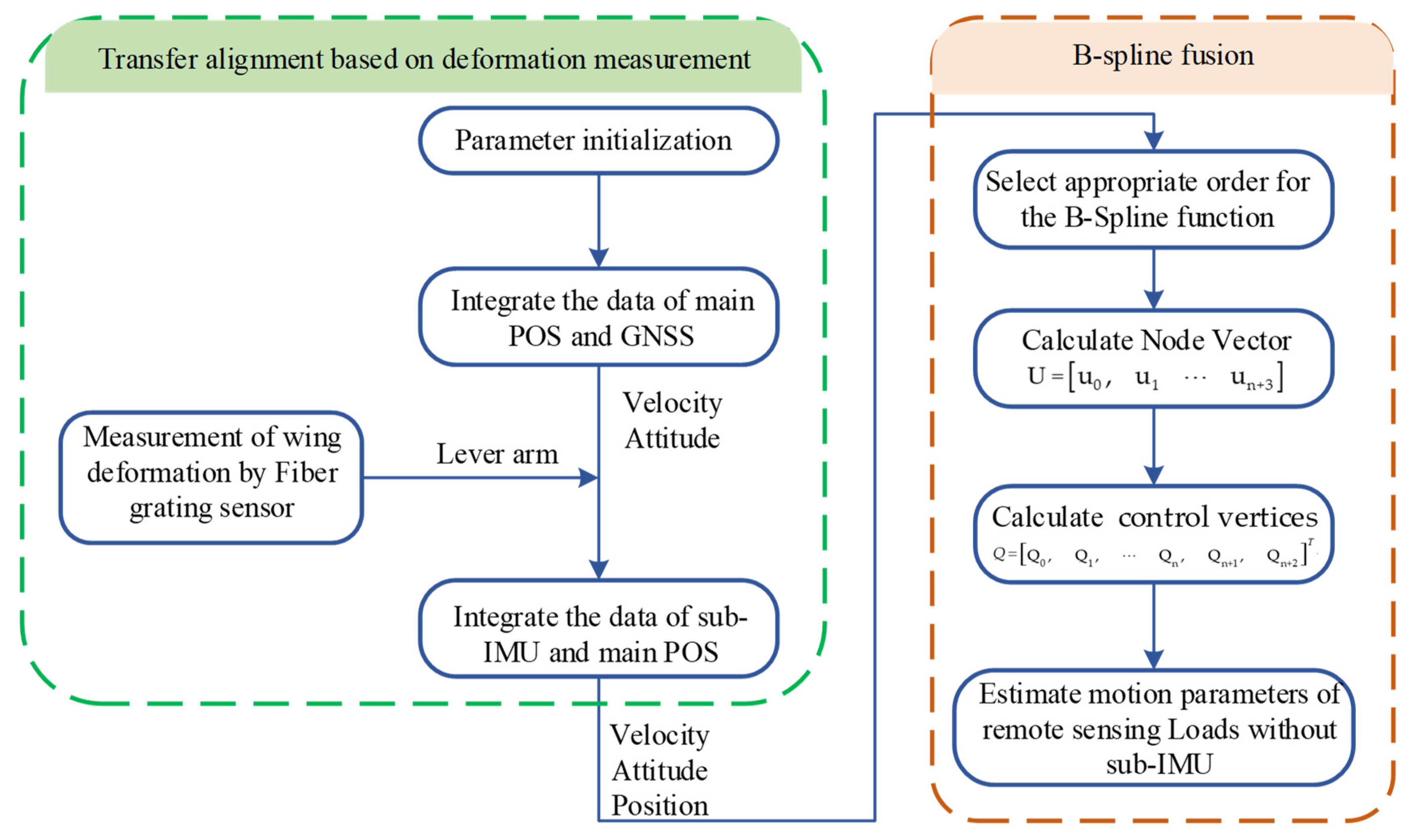
Then, combined with the node vector obtained in 3.1, the B-spline function of the wing is constructed. At last, a flow chart of the transmission alignment based on fiber-grating compensation introduced in Section 2 and the B-spline interpolation introduced in Section 3 is shown in Figure 4.

3. Results

3.1. Experimental Equipment

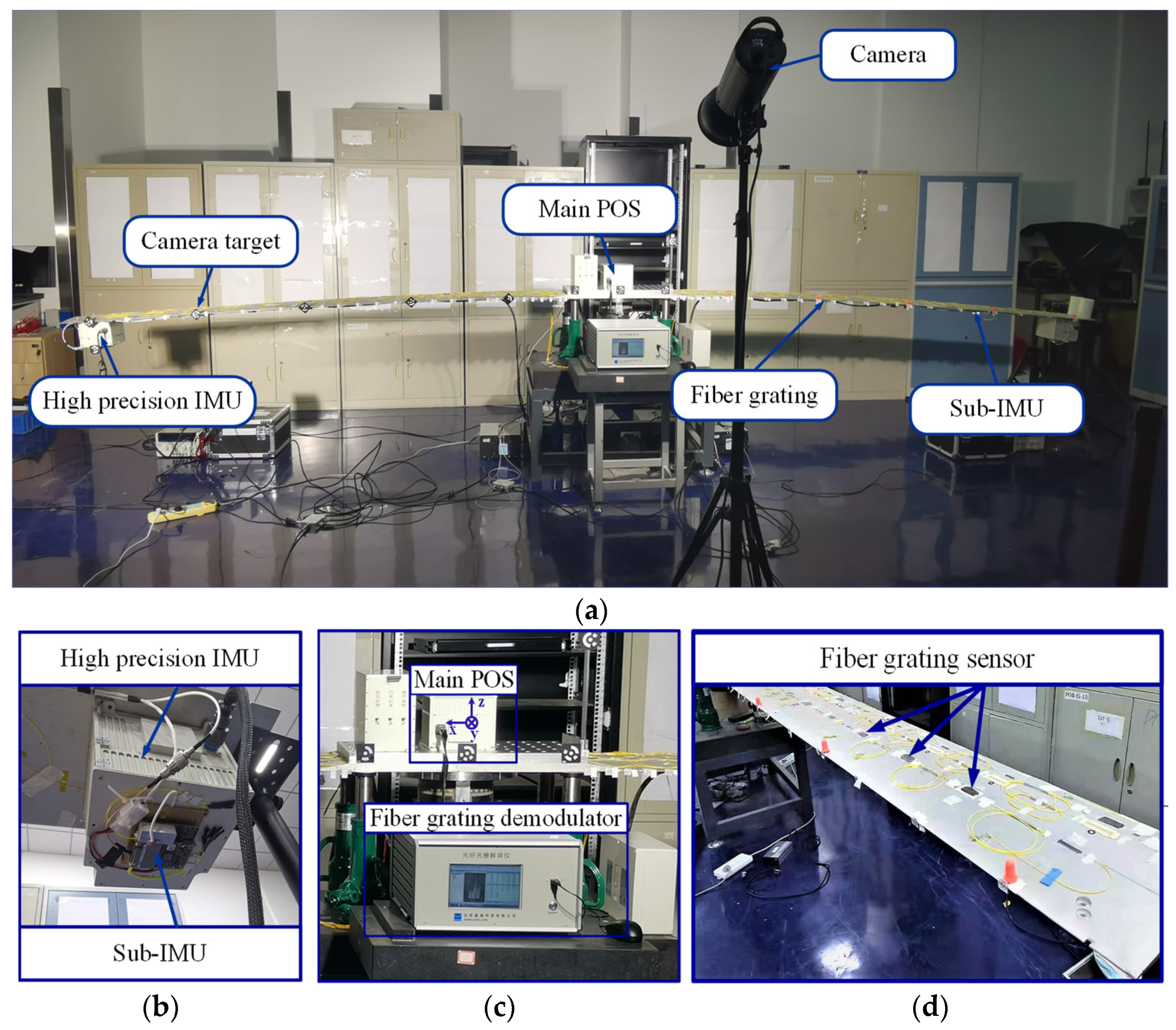
As mentioned above, to further improve the measurement accuracy of the array POS, the alignment results of multiple sub-IMUs are fused by the B-spline fusion with full use of the spatial correlation of each sub-IMU. To validate the performance of the proposed method, a semi-physical simulation based on ground experiments is conducted, which is described in detail below. The airborne array POS ground experimental system based on fiber Bragg grating mainly includes a simulated wing, a fiber-grating deformation measurement system, an array POS measurement system and a high-precision binocular camera, as shown in Figure 5. Figure 5a is the overall layout of the experiment, which mainly includes the array POS, high-precision binocular camera, and camera targets. The data measured with high-precision cameras can be used as the position reference. Figure 5b shows the high-precision IMU and the fixed-link sub-IMU. The data measured with the high-precision IMU can be used as the position and attitude reference. Figure 5c shows the main POS and unified coordinate system. The installation layout of the fiber-optic grating sensors is shown in Figure 5d.
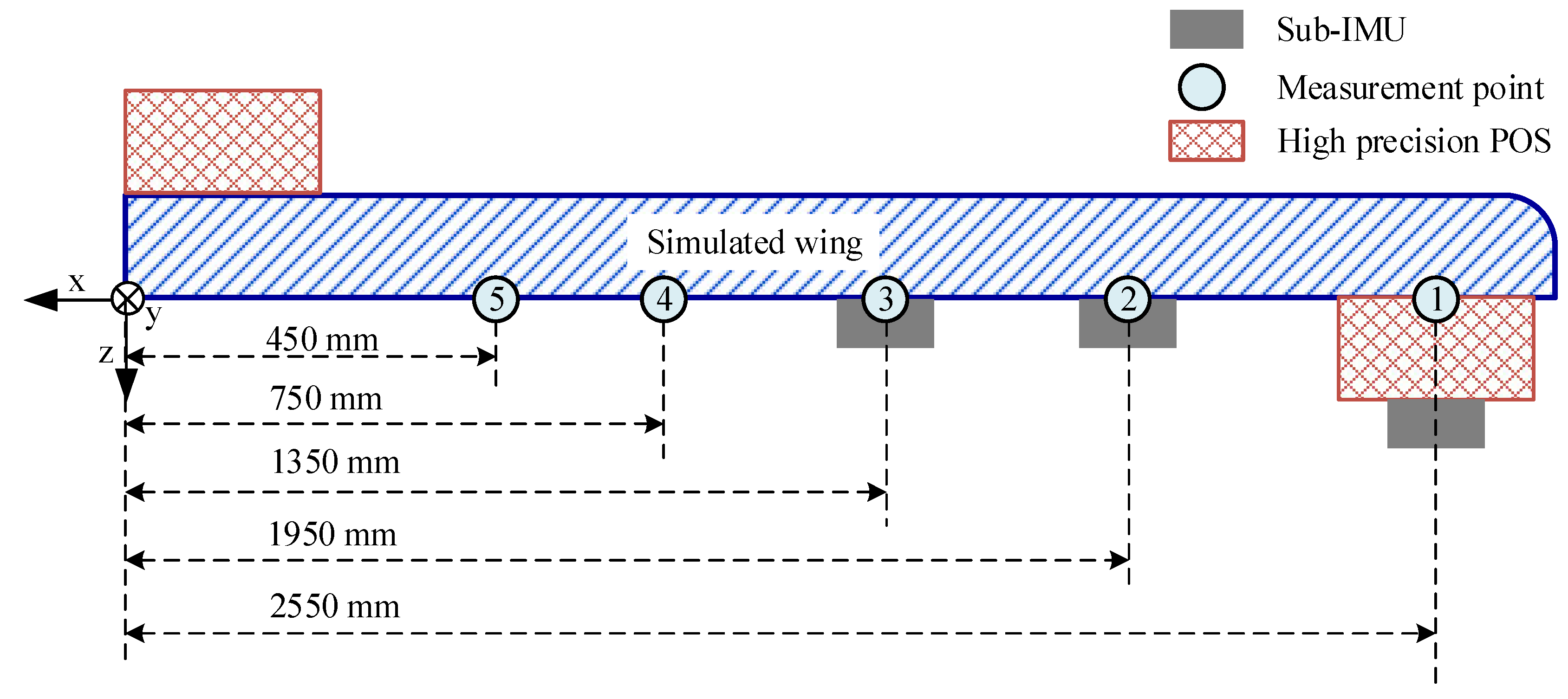
As shown in Figure 5, the simulated wing has bilateral symmetry, and the length of the unilateral wing is 3000 mm. The upper surface of the simulated wing shape is streamlined with reference to the real wing shape, while the lower surface of the simulated wing is flat and convex, which meets the requirements of sensor plane installation. The fiber-grating sensor is installed on the surface of the wing. The main POS is installed in the center of the wing, which is composed of high-precision optical fiber IMU, the GNSS receiver and the integrated navigation computer, which can accurately measure the position, speed, attitude and other motion information of the main antenna in real time. The sub-IMU is an inertial measurement system based on Micro-Electro-Mechanical System, and sub-IMUs are distributed on the measuring points of the wing. The critical parameter indices of the main POS and sub-IMUs are shown in Table 1. There are five measuring points on the unilateral wing. Measuring point 1 is 2550 mm away from the main POS and is located at the end of the wing. The distances from the other four measuring point to the main POS are 1950 mm, 1350 mm, 750 mm and 450 mm, respectively. The locations of the measuring points are shown in Figure 6. Due to the number limitation of the system, sub-IMUs are installed at measuring points 1 to 3 of the unilateral wing. The high-precision binocular camera is located on the ground in front of the simulated wing, which provides high-precision position reference for the measuring points. Additionally, a high-precision optical fiber POS is also installed at measuring point 1 on the left and right sides of the simulated wing, which is rigidly connected with the sub-IMU. The transfer alignment result of the high-precision optical fiber POS can provide attitude reference for measuring point 1.
Before the experiment, the IMUs are installed according to the positions shown in Figure 5, and the connectors and power supply are checked. Then the Fiber Bragg Grating Sensor and Fiber Bragg Grating Demodulator shown in Figure 4 are connected, the data collection frequency of which is set to 20 Hz to collect and save data. After all sensors are installed, the simulated wing remains stationary without any loads. The end of the wing is supported to achieve a straight state. The micrometer is set to zero and placed at a predetermined measuring point to calibrate the data of the fiber-grating sensor. The wing support is removed before the experiment to make the wing sag naturally. Loads of 1 kg, 3 kg and 5 kg are successively loaded to the end of the wing during the test, to simulate the influence of different external environments on the wing deformation. The time interval for applying different loads is 4 min. The load is removed when the wing is stable, and the data are recorded during the experiment.

3.2. Experiment Results

After the experiment, the data are processed. Firstly, the master—slave transfer alignment is performed. The transfer alignment method assisted by fiber Bragg grating is applied and the position and posture matching mode is selected. After that the motion information of the IMU at measurement point 1, measurement point 2 and measurement point 3 can be obtained, and the results can be used in the global information fusion. Secondly, the estimation method based on B-spline is carried out, after which the motion information of each node at the wing can be obtained. Namely, the baseline distance and roll attitude information of the corresponding nodes are obtained, which is the motion information vector difference between the main and sub-IMUs. During aircraft flight, the imaging quality of the remote-sensing payload is most affected by the baseline and roll angle in the z-axis direction [26]. Due to space limitations, the fusion results of the baseline and roll angle are selected as evaluation indicators in this paper.
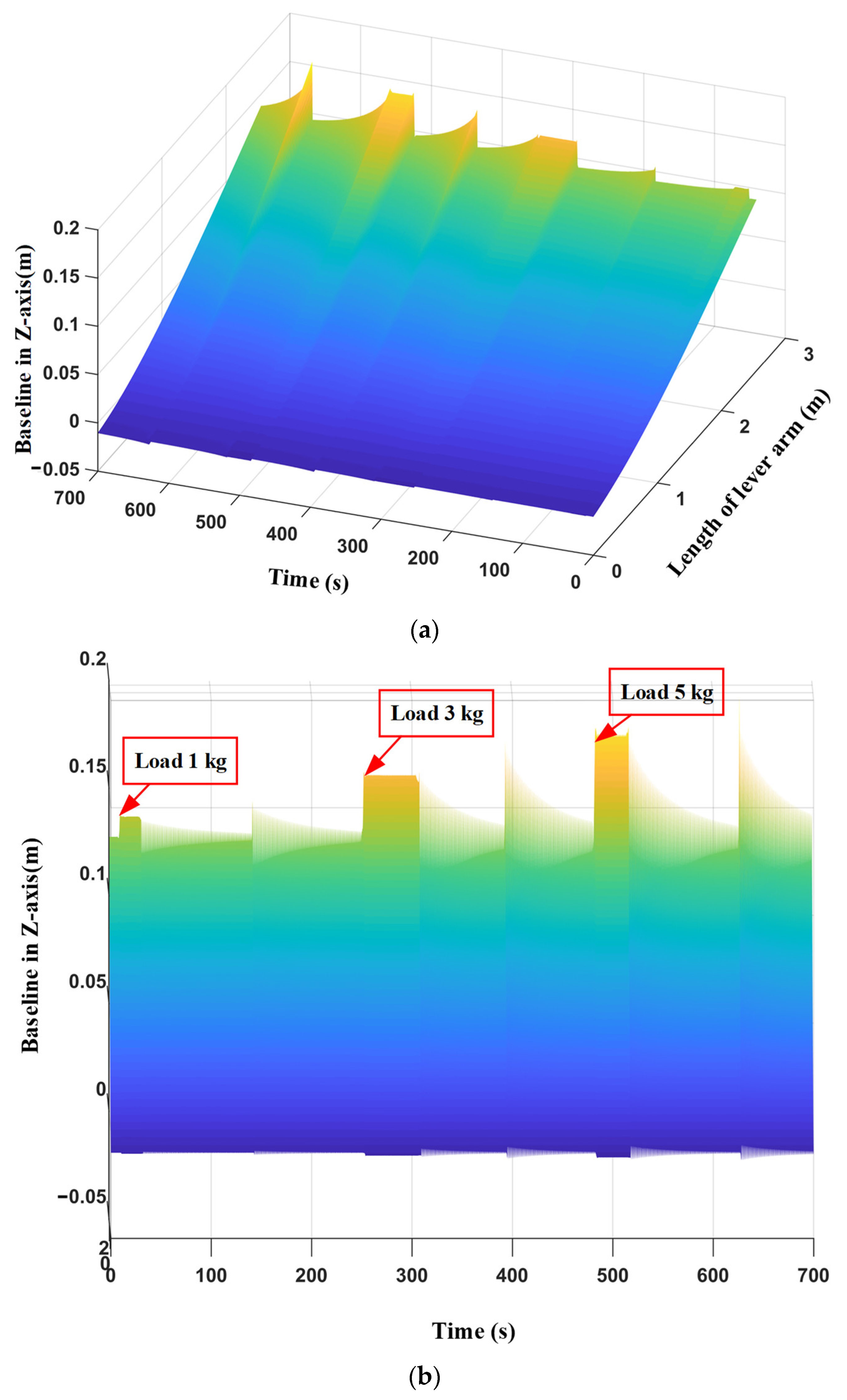
Figure 7 shows the baseline B-spline fusion result in the Z-axis. It can be seen in Figure 7 that the baseline in the Z-axis direction increases with the length of the lever arm and the load weight. When the load is 1 kg, the maximum baseline of the Z-axis direction is 0.131 m. When the load is 3 kg, the maximum baseline of the Z-axis direction is 0.152 m, and when the load is 5 kg, the maximum baseline of the Z-axis direction is 0.173 m. And the maximum baselines are all obtained when the length of the lever arm is longest. The fitting results of the baseline at measuring point 1 are taken to verify the correctness of the proposed method. The post-processing results of the high-precision IMU are used as benchmarks. The baseline fitting results are shown in Figure 8.
Table 2 shows the accuracy of the baseline error. RMSE is selected as the error statistics method in this section. It can be seen in Figure 8 and Table 2 that the baseline error in the Y-axis is minimal and the baseline error in the X-axis is the largest. When the load is 1 kg, the baseline errors obtained by the B-spline fusion in the X-axis, Y-axis and Z-axis are 5.748 mm, 0.531 mm and 3.987 mm, respectively, which are improved by 7.68%, 17.16% and 21.35% compared to that obtained by the transfer alignment. When the load is 3 kg, the baseline error obtained by the B-spline fusion in the X-axis, Y-axis and Z-axis are 5.013 mm, 0.617 mm and 4.164 mm, respectively, which are improved by 6.89%, 19.03% and 21.32% compared to that obtained by the transfer alignment. When the load is 5 kg, the baseline error obtained by the B-spline fusion in the X-axis, Y-axis and Z-axis are 6.594 mm, 0.683 mm and 4.302 mm, respectively, which are improved by 8.37%, 18.59% and 22.79% compared to that obtained by the transfer alignment. The baseline in the X-axis, Y-axis and Z-axis are improved 0.484 mm, 0.137 mm and 1.225 mm, respectively.
The roll angle B-spline fusion result of each node is shown in Figure 9. It can be seen in the figure that the roll angle increases with the length of the lever arm and the load weight. When the load is 1 kg, the maximum roll angle is 4.581°. When the load is 3 kg, the maximum roll angle is 5.687°. When the load is 5 kg, the maximum roll angle is 6.508°. And the maximum roll angles are all obtained when the length of the lever arm is longest.
Figure 10 shows the accuracy comparison of the roll angle at measurement point 1 before and after fusion. The transfer alignment result is represented by the blue line, while the B-spline fusion result is represented by the rose line. It can be seen in Figure 9 that, after B-spline fusion, the accuracy of the roll angle is improved regardless of the load weight. The maximum roll angle errors of the transfer alignment results are 0.121°, 0.311° and 0.383°, respectively, when the loads are 1 kg, 3 kg and 5 kg, while the maximum roll angle errors of the B-spline fusion results are 0.104°, 0.270° and 0.347°, respectively, when the load are 1 kg, 3 kg and 5 kg.
Table 3 shows the RMSE accuracy of the roll angle at measurement point 1. It can be seen in Table 3 that the accuracy of the B-spline fusion is higher than that of the transfer alignment result. The roll angle accuracy obtained by the B-spline fusion is improved by 31.25%, 27.08% and 28.07%, respectively, compared to that obtained by the transfer alignment, when the loads are 1 kg, 3 kg and 5 kg. And the average measurement accuracy of the roll angle is improved from 0.040° to 0.029°, which indicates that the continuous correlation of motion information of all sub nodes can be fully utilized in the B-spline fusion to effectively improve the estimation accuracy of the array POS.

4. Conclusions and Discussion

The array POS with multiple sub-IMUs can provide motion compensation for multi-task remote-sensing loads, so it is key equipment in aviation remote-sensing systems. However, due to the volume, weight, cost and other factors, it is impossible to equip each remote-sensing load with a sub-IMU. To obtain the motion parameters of the remote-sensing loads without sub-IMU, an estimation method based on the B-spline fusion is introduced in this paper. At first, the transfer alignment model based on fiber-grating compensation for the combined inertial navigation mode of one master and multiple sub-IMUs in an array POS is built, which can obtain the motion parameters of the remote-sensing loads equipped with sub-IMUs. And then, the estimation model based on the B-spline fusion is described in detail to obtain the motion information of the remote-sensing loads without sub-IMUs. At last, to verify the effectiveness of the proposed method, a semi-physical simulation based on a ground-loading test is conducted. Different loads are applied to the end of the wing to simulate the deformation of the wing under different conditions. The measurement accuracy of the baseline and roll angle, which have a significant impact on imaging quality, are selected as the evaluation indicators. The results show that the proposed method obtains better estimation performance compared with transfer alignment. However, there are limitations to the present study. The main limitation is the experimental equipment. The array POS is mainly used in the field of aerial remote sensing. The higher the performance of aerial remote sensing, the more antennas required, and the longer baseline needed, which leads to a more significant flexible baseline effect. The estimation method is suitable for situations where the flexible baseline effect is significant. However, the wings of existing aircraft are usually rigid, which is does not apply to the situation of flexible long wings. It requires coordination among many departments and a large amount of manpower material and financial resources to modify an aircraft. The wing used in the ground-loading test can effectively simulate flexible long wings. Yet the real flight test environment is relatively harsh. Wing deformation can be caused by lots of factors such as gusts, turbulence and engine vibration during flight. The characteristics of wing deformation caused by different factors are different. Different loads are loaded on the end of the wing in this paper to simulate wing deformation under different conditions, which may not truly reflect the deformation of the wing during actual flight and requires further research in the future. In spite of the limitations, limited sub-IMUs used in this study can achieve motion compensation for infinite remote-sensing loads, by which the applicability of an array POS is improved. With the estimation method mentioned in this article, it is also worth researching in the future how to achieve motion compensation with fewer sub-IMUs, which is of great significance in saving costs and reducing the weight of the carrier.
It is worth pointing out that the velocity of the ground experiment is limited and not representative, so it is not stated in this paper. And the methods mentioned in this paper are conducted on MATLAB in the current implementation, which will be replaced by C++ in the future to improve real-time performance.

Author Contributions

Conceptualization, J.B. and J.L.; methodology, J.B.; software, J.B.; validation, J.B. and J.L.; formal analysis, J.B. and J.L.; investigation, J.L. and Y.L.; resources, J.L.; data curation, J.L.; writing—original draft preparation, J.B.; writing—review and editing, J.B., J.L. and C.Q.; visualization, J.B., J.L., C.Q. and Y.L.; supervision, J.L.; project administration, J.L.; funding acquisition, J.L. All authors have read and agreed to the published version of the manuscript.

Funding

This research was funded by the Innovation program for Quantum Science and Technology, 2021ZD0300403 and Natural Science Foundation for Distinguished Young Scholars, Grant 62225102.

Data Availability Statement

Not applicable.

Conflicts of Interest

The authors declare no conflict of interest.

References

  1. Montgomery, J.; Mahoney, C.; Brisco, B. Remote Sensing of Wetlands in the Prairie Pothole Region of North America. Remote Sens. 2021, 13, 3878. [Google Scholar]
  2. Tsokas, A.; Rysz, M.; Pardalos, P. SAR Data Applications in Earth Observation: An Overview. Expert Syst. Appl. 2022, 205, 117342. [Google Scholar]
  3. Chen, L.; Liu, Z.; Fang, J. An Accurate Motion Compensation for SAR Imagery based on INS/GPS with Dual-filter Correction. J. Navig. 2019, 72, 1399–1416. [Google Scholar]
  4. Zhang, B.; Yu, A.; Chen, X. Comparative Analysis of Single-View and Multi-View Airborne SAR Positioning Error and Course Planning for Multi-View Airborne SAR Optimal Positioning. Remote Sens. 2022, 14, 3055. [Google Scholar]
  5. Qu, C.; Li, J.; Bao, J.; Zhu, Z. Design and Development of Array POS for Airborne Remote Sensing Motion Compensation. Remote Sens. 2022, 14, 3420. [Google Scholar] [CrossRef]
  6. Wang, J.; Liang, X.; Ding, C.; Chen, L.; Wang, Z.; Li, K. A novel scheme for ambiguous energy suppression in MIMO-SAR systems. IEEE Geosci. Remote Sens. Lett. 2015, 12, 344–348. [Google Scholar]
  7. Gong, X.L.; Ding, X.S. Adaptive CDKF Based on Gradient Descent with Momentum and its Application to POS. IEEE Sens. J. 2021, 21, 16201–16212. [Google Scholar]
  8. Ye, W.; Liu, Z.; Li, C.; Fang, J. Enhanced Kalman Filter using Noisy Input Gaussian Process Regression for Bridging GPS Outages in a POS. J. Navig. 2018, 71, 565–584. [Google Scholar]
  9. Qu, C.; Li, J. A novel relative motion measurement method based on distributed POS relative parameters matching transfer alignment. Measurement 2022, 202, 111890. [Google Scholar] [CrossRef]
  10. Ye, W.; Li, J.; Li, L. Design and development of a real-time multi-DSPs and FPGA-based DPOS for InSAR applications. IEEE Sens. J. 2018, 18, 3419–3425. [Google Scholar]
  11. Li, J.; Jia, L.; Liu, G. Multisensor Time Synchronization Error Modeling and Compensation Method for Distributed POS. IEEE Trans. Instrum. Meas. 2016, 65, 2637–2645. [Google Scholar]
  12. Bao, J.; Li, J.; Wei, M.; Qu, C. An Improved Innovation Robust Outliers Detection Method for Airborne Array Position and Orientation Measurement System. Remote Sens. 2023, 15, 26. [Google Scholar] [CrossRef]
  13. Li, J.; Qu, C. A Novel Transfer Alignment Method of Array POS Based on Lever-arm Estimation. IEEE Trans. Instrum. Meas. 2022, 71, 1–11. [Google Scholar]
  14. Li, J.; Qu, C.; Zhu, Z. Six-Dimensional Deformation Measurement of Distributed POS Based on FBG Sensors. IEEE Sens. J. 2021, 21, 7849–7856. [Google Scholar]
  15. Ye, W.; Li, J.; Fang, J. EGP-CDKF for Performance Improvement of the SINS/GNSS Integrated System. IEEE Trans. Ind. Electron. 2018, 65, 3601–3609. [Google Scholar]
  16. Liu, Y.; Wang, B.; Ning, L.; Gu, B. Global Estimation Method Based on Spatial–Temporal Kalman Filter for DPOS. IEEE Sens. J. 2021, 21, 3748–3756. [Google Scholar]
  17. Wang, G.; Xu, X.; Yao, Y. A Novel BPNN-based method to overcome the GPS Outages for INS/GPS system. IEEE Access 2019, 7, 82134–82143. [Google Scholar]
  18. Wei, X.; Li, J.; Feng, K.; Zhang, D.; Li, P.; Zhao, L.; Jiao, Y. A Mixed Optimization Method Based on Adaptive Kalman Filter and Wavelet Neural Network for INS/GPS During GPS Outages. IEEE Access 2021, 9, 47875–47886. [Google Scholar]
  19. Liu, C.; Liu, Z.; Han, X. Preconditioned progressive iterative approximation for tensor product Bézier patches. Math. Comput. Simul. 2021, 185, 372–383. [Google Scholar]
  20. Hamza, Y.; Lin, H.; Li, Z. Implicit progressive-iterative approximation for curve and surface reconstruction. Comput. Aided Geom. Des. 2020, 77, 101817. [Google Scholar]
  21. Zheng, R.; Chen, C.; Yang, G. Deck deformation measurement of large-sized ship based on LSE. J. Harbin Inst. Technol. 2009, 41, 141–144. [Google Scholar]
  22. Gong, X.; Liu, H.; Fang, J.; Liu, G. Multi-Node Transfer Alignment Based on Mechanics Modeling for Airborne DPOS. IEEE Sens. J. 2018, 18, 669–6799. [Google Scholar]
  23. Wang, J.; Zhang, A.; Meng, X. Super-resolution reconstruction of remote sensing image based on staggered pixels and non-uniform B-spline curved surface. Remote Sens. Land Resour. 2015, 27, 35–43. [Google Scholar]
  24. Gawali, D.; Patil, B.V.; Zidna, A. Constrained global optimization of multivariate polynomials using polynomial B-spline form and B-spline consistency prune approach. RAIRO-Oper. Res. 2021, 55, 3743–3771. [Google Scholar]
  25. Peng, R. Non-Ellipsoidal Infrared Group/Extended Target Tracking Based on Poisson Multi-Bernoulli Mixture Filter and B-Spline. Remote Sens. 2023, 15, 606. [Google Scholar]
  26. Ding, Z.; Tan, W.; Wang, Y.; Hong, W.; Wu, Y. Impact analysis of motion measurement error on array antenna SAR three dimensional imaging. J. Electron. Inf. Technol. 2015, 37, 1424–1430. [Google Scholar]
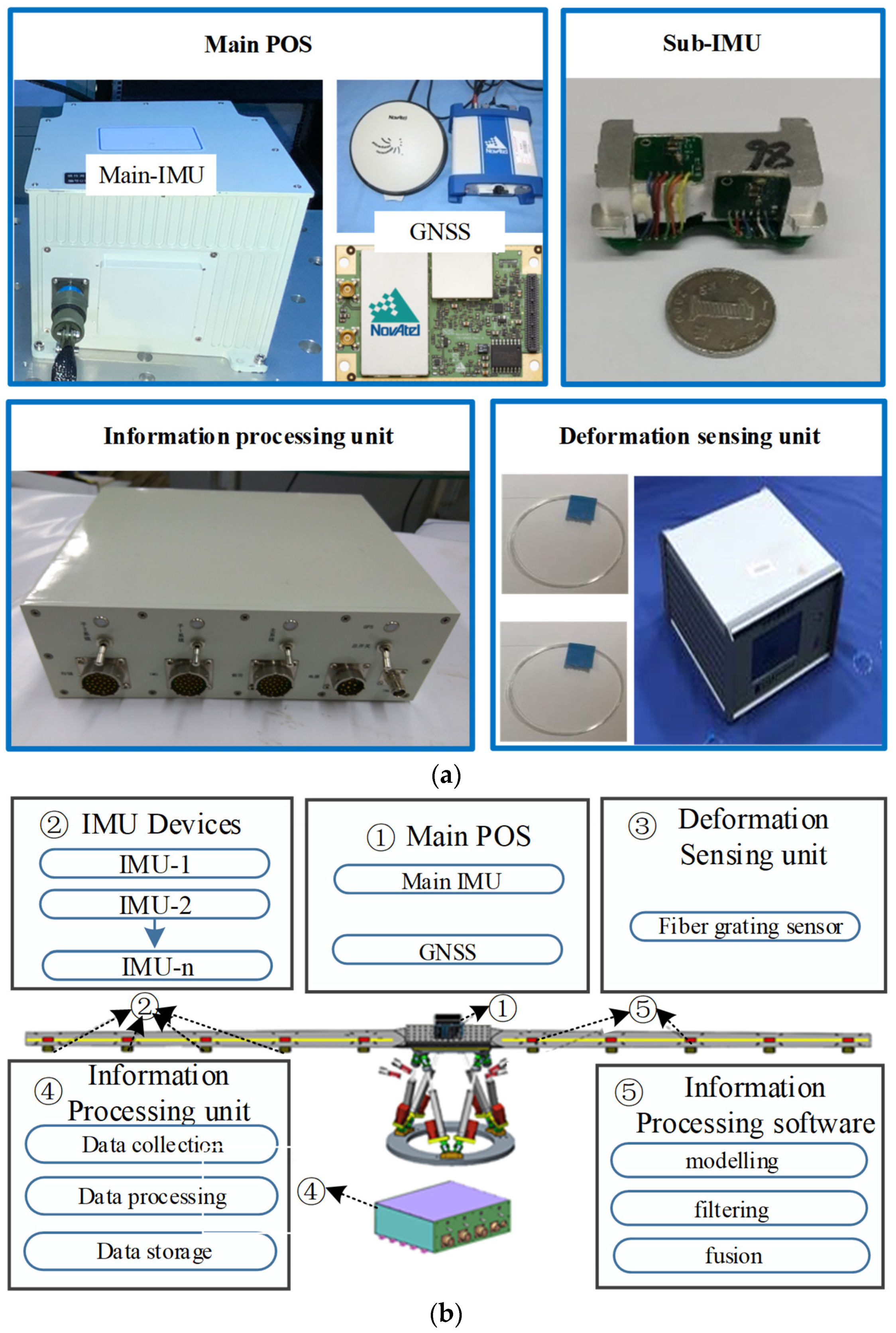
Figure 1. Component of the array POS and IMU system. (a) Physical composition; (b) diagram of the array POS and IMU system.
Remotesensing 15 02892 g001
Figure 2. The main coordinate frames.
Remotesensing 15 02892 g002
Figure 3. Lever arm between main POS and sub-IMU.
Remotesensing 15 02892 g003
Figure 4. Flow diagram of the transfer alignment and the B-spline fusion.
Remotesensing 15 02892 g004
Figure 5. Installation layout of the array POS. (a) Installation layout of the array POS; (b) High-precision POS and fixed-link IMU; (c) Main POS and unified coordinate system; (d) Physical installation drawing of fiber grating.
Remotesensing 15 02892 g005
Figure 6. Installation diagram of the array POS ground experiment of the unilateral simulated wing.
Remotesensing 15 02892 g006
Figure 7. Baseline in Z-axis B-spline fusion results of each node. (a) Stereogram; (b) Plane.
Remotesensing 15 02892 g007
Figure 8. Baseline error.
Remotesensing 15 02892 g008
Figure 9. Roll Angles B-spline fusion Results of Each Node. (a) Stereogram; (b) Plane.
Remotesensing 15 02892 g009
Figure 10. Comparison of roll angle error results at measurement point 1.
Remotesensing 15 02892 g010
Table 1. The critical parameter indices of the main POS and sub-IMU.
ParametersIndex
Gyro drift of main POS0.01°/h
Accelerometer bias of main POS20 μg
Gyro drift of sub-IMU5°/h
Accelerometers random of sub-IMU50 μg
Table 2. RMSE accuracy of relative position (mm).
Accuracy (STD)Baseline in X-AxisBaseline in Y-AxisBaseline in Z-Axis
Transfer Alignment
Result
B-Spline
Fusion
Result
Transfer Alignment
Result
B-Spline
Fusion
Result
Transfer Alignment
Result
B-Spline
Fusion
Result
Load 1 kg6.2265.7480.6410.5315.0693.987
Load 3 kg5.3845.0130.7620.6175.2924.164
Load 5 kg7.1976.5940.8390.6835.4674.302
Average6.2695.7850.7470.6105.3764.151
Table 3. RMSE accuracy of roll angle.
Accuracy (STD)Measuring Point 1
Transfer Alignment
Result
B-Spline Fusion
Result
load 1 kg 0.016°0.011°
load 3 kg 0.048°0.035°
load 5 kg 0.057°0.041°
Average 0.040°0.029°
Disclaimer/Publisher’s Note: The statements, opinions and data contained in all publications are solely those of the individual author(s) and contributor(s) and not of MDPI and/or the editor(s). MDPI and/or the editor(s) disclaim responsibility for any injury to people or property resulting from any ideas, methods, instructions or products referred to in the content.