Article

Retrieval of Atmospheric Temperature Profile from Historical Data and Ground-Based Observations by Using a Machine Learning Algorithm

1
Institutes of Physical Science and Information Technology, Anhui University, Hefei 230601, China
2
Key Laboratory of Atmospheric Optics, Anhui Institute of Optics and Fine Mechanics, Chinese Academy of Sciences, Hefei 230088, China
3
Science Island Branch of Graduate School, University of Science and Technology of China, Hefei 230026, China
4
Opto-Electronics Applied Technology Research Center, Anhui Institute of Optics and Fine Mechanics, Chinese Academy of Sciences, Hefei 230031, China
*
Author to whom correspondence should be addressed.
Remote Sens. 2023, 15(11), 2717; https://doi.org/10.3390/rs15112717
Submission received: 7 March 2023 / Revised: 17 May 2023 / Accepted: 18 May 2023 / Published: 24 May 2023
(This article belongs to the Section Atmospheric Remote Sensing)

Abstract

:
The atmospheric temperature profile is an important parameter to describe the state of the atmosphere, and it is crucial to climate change research, weather forecasting, and atmospheric parameter retrieval. A machine learning algorithm that incorporates historical observations and ground-based measurements was developed in this study to retrieve the atmospheric temperature profile. Specifically, the deep learning network considered historical observations for the same period and temporally correlated temperature profiles. It combined multi-layer perceptron (MLP) and the convolutional neural network (CNN). MLP derived the features from the ground factors, and CNN captured the essential features associated with the temperature profiles at the current time from latent historical data. Then, the features of the two parts were concatenated to obtain the final network. The construction and parameters of the model were optimized to determine the best model configuration and retrieval performance. The results of the model were evaluated against those of other methods on the same dataset. The model showed a good retrieval precision, which was equivalent to a small retrieval bias, root-mean-square error, and mean absolute error at all altitudes. The analysis of the application of this model to the retrieval of atmospheric temperature profiles indicates that the method is feasible.

Graphical Abstract

1. Introduction

The atmospheric temperature profile which describes the distribution of temperature in the atmosphere with height is an essential parameter to describe the thermodynamic state of the atmosphere, and it is crucial to numerous practical and scientific applications, such as numeric weather prediction and climate studies [1,2,3]. The accuracy of global temperature and humidity detection must reach the radiosonde level to fulfil the observational requirements of the World Meteorological Organization, which indicates that the profiles of tropospheric atmospheric temperature should be derived with a root-mean-square error (RMSE) of less than 1 °C and a final vertical resolution of 1 km [4,5]. Atmospheric profiles including atmospheric temperature profile are widely used in the research on radiative transfer models and atmospheric parameter retrieval [6].
The widely applied atmospheric radiative transfer calculation models include LBLRTM [7], FASCOD [8], LOWTRAN [9], and MODTRAN [10,11]. These calculation models require the input of atmospheric temperature profiles, which are typically represented by a subset of the 1966 Atmospheric Supplements (tropical [15N], middle latitude’ [45N] summer and winter, and subarctic [60N] summer and winter) and the U.S. Standard Model Atmosphere (1976) [12]. Practical temperature profiles vary greatly with regions and seasons [13], which means the spatiotemporal distribution is not fully represented by climatological temperature profiles. Errors may occur when climatological temperature profiles are used for model calculation and atmospheric parameter retrieval [14]. Temperature profiles need to be in line with local conditions and must have real-time capability to perform well in atmospheric radiative transfer calculation.
Therefore, research on real-time temperature profile measurement and local atmospheric temperature profile models can support the application of atmosphere samples in studies on radiative transfer and remote sensing retrieval [15]. The radiosonde is the traditional tool for measuring temperature profiles. By using radiosondes, meteorological departments can obtain the accurate distribution of atmospheric temperature and other profiles directly. However, problems still arise when radiosondes are employed to measure atmospheric temperature profiles. The results of radiosonde method are observed at certain geographical locations every 12 h. Radiosonde detection technology lacks temporal and spatial resolution and has significant disadvantages in terms of global coverage and continuous long-term measurement [2,16].
The extensive requirement on temperature information for continuous spatiotemporal observations of global and regional atmospheric features has made remote sensing an important measurement. Remote sensing facilitates the development of meteorological and atmospheric science research and applications [17]. Remote sensing techniques for detecting tropospheric atmospheric temperature profiles can be divided into two types, namely, active and passive, depending on the detection mode. Each technique has its advantages in terms of vertical resolution and sensitivity to the boundary layer atmosphere [18,19]. The representative equipment of active remote sensing observations is lidar, which uses laser as the light source. Lidar studies the structure of the atmosphere by detecting the signal generated by the interaction between the laser and the target [20]. It was widely used in the measurement of the spatial distribution and time evolution characteristics of atmospheric temperature. Lidar can detect atmospheric parameter profiles with high temporal and spatial resolutions compared with traditional radiosondes [3,21,22]. The research on tropospheric atmospheric temperature focused on pure rotational Raman lidar. This type of lidar is designed to measure atmospheric temperature based on the dependence of the atmosphere molecular rotational Raman spectral envelope on temperature. Given the increasing research on atmospheric temperature detection, pure rotational Raman lidar became one of valid methods of profiling atmospheric temperature [22,23,24]. The representative equipment of passive remote sensing observations are microwave radiometers and infrared hyperspectral sensors. Passive remote sensing refers to the technology or method wherein the remote sensing equipment receives electromagnetic radiation emitted by the atmosphere or reflects electromagnetic radiation from natural sources to obtain atmospheric information [19]. Microwave radiometers receive atmospheric thermal radiation to retrieve the atmospheric temperature and humidity profile from multi-channel brightness temperature data [19,25]. Microwave radiometers have many advantages, such as simple operation, not being limited by airspace, and high time resolution. They became important instruments and are widely used in atmospheric profile remote sensing detection [26,27,28]. Many studies [28,29,30] showed that passive microwave data can be used to retrieve atmospheric temperature with strong validity. Infrared hyperspectral remote sensing detection retrieves the atmospheric temperature and humidity profile from CO2 and H2O absorption bands in infrared spectral bands [18,31,32]. This method can obtain a highly detailed atmospheric structure and improve the ability and accuracy of detecting the atmosphere [33,34].
Studies [18,21,25,35,36] showed that the main retrieval methods related to passive remote sensing can be divided into two types: statistical regression and physical methods. With the development of artificial intelligence technology, machine learning algorithms were gradually introduced into the field of atmospheric science [33]. Studies [34,37,38,39] also showed that neural networks have better performance than traditional methods in the retrieval of temperature profiles. Remote sensing methods have their advantages and disadvantages. They all have high resolution and accuracy, but they are greatly influenced by high equipment costs. In practical applications, when remote sensing devices are unavailable, historical observations can be used to obtain atmospheric temperature profiles. A study [40] reported that the addition of surface temperature factors helps improve the inversion results. Qin et al. (2003) [41] proposed a model based on historical radiosonde and real-time ground data. The model combined the local month-by-month average temperature profile and the surface temperature to obtain the temperature profile at any moment through the interpolation of scale factors. However, only 12 monthly average temperature profiles can be obtained without considering the hourly temperature profile changes in a day. At the same time, the ground-based parameters only included the surface temperature and disregarded other parameters, such as atmospheric pressure, humidity, and total cloud cover.
To improve on the limitations of remote sensing, including limitations in the cost of building equipment, limitations in the spatial and temporal scope of measurements, and other disadvantages, a neural network that combines multi-layer perceptron (MLP) and convolutional neural network (CNN) is proposed to retrieve atmospheric temperature profiles. This study analyzes the time characteristics of the temperature profiles and potential information characterized by different ground-based parameters to improve the retrieval accuracy from historical and ground-based observations. This approach is also compared against several different model-based methods for retrieving atmospheric temperature profiles. The practical use of the proposed network construction method is demonstrated herein for retrieving temperature profiles in Fuyang city.

2. Data Introduction

2.1. Study Region

Fuyang City is located at the southern end of the Yellow Huaihai Plain, the western part of the Huabei Plain and the northwestern part of Anhui Province, with a total area of 10,118.2 square km. It extends from 114°52′E to 116°49′E and from 32°25′N to 34°04′N. The whole area is a plain with a flat topography, high in the northwest and low in the southeast, slightly sloping from northwest to southeast, with a relative slope of 14.4 m between northwest and southeast. Fuyang is located on the southern edge of the warm temperate zone and has a warm temperate semi-humid monsoon climate. The monsoon is obvious, the seasons are distinct, the climate is mild, and the rainfall is moderate. It also has the characteristics of a transitional zone climate with gradual changes from the warm temperate zone to the northern subtropical zone. The Fuyang National High Altitude Meteorological Observatory is located in Fuyang City. The study area was chosen because of the uniform and flat topography of the area with four distinct seasons.

2.2. ERA-5 Data

This study was based on ERA-5 data of Anhui Province ranging from 32°N to 33°N and 115°E to 116°E from 2001 to 2021. The training and testing data were obtained from the ERA-5 data (70-year ERA starting from January 1950 onward with timely updates) of the European Centre for Medium-Range Weather Forecast, which provides the most accurate global numerical model predictions [42]. ERA-5 data make up the fifth generation of atmospheric reanalysis produced for global climate and weather, and they replace ERA-Interim (40-year ERA from January 1979 to August 2019) reanalysis due to their higher temporal and spatial resolutions [43]. Many studies already applied ERA-5 reanalysis data with effectively evaluated credibility and applicability [44,45,46]. ERA-5 data use observations from a wide range of satellite instruments or conventional data types. For example, high-altitude observations of wind, temperature, and humidity were obtained from pilots, radio sounders, down-dropping sounders, and aircraft measurements, and many other data in ERA-5 were derived from measurements from many satellite platforms. The data contained ERA-5 hourly information on pressure levels and ERA-5 hourly information on single levels. All temperature profile data and ground-based meteorological data were averaged over the region, and the model was trained and analyzed on the average data. The hourly data are available on the C3S Climate Data Store cloud server (https://cds.climate.copernicus.eu/; accessed on 11 April 2020) [43]. The upper-air parameters of ERA-5 reanalysis data had a high horizontal resolution of 0.25° × 0.25° and contained information on the atmosphere at 37 altitudes. The atmosphere parameters in this study included 27 layers from 1000 hPa to 100 hPa (the pressure for each layer was set as follows: 1000, 975, 950, 925, 900, 875, 850, 825, 800, 775, 750, 700, 650, 600, 550, 500, 450, 400, 350, 300, 250, 225, 200, 175, 150, 125, and 100 hPa) of atmospheric temperature information. The surface parameters included 2 m temperature, 2 m relative humidity, surface pressure, 10 m u-component of wind, 10 m v-component of wind, and total cloud cover. The description of the ERA-5 data used in this study is shown in Table 1, and the main variables of the ERA-5 surface data are shown in Table 2.

3. Method

3.1. Data Pre-Processing

The ERA-5 reanalysis data had to be pre-processed. Since the data types contained surface observations and pressure-distributed temperature data, the two data components were synchronized in time. The surface observations were used as input and the pressure-distributed temperature data as output in the deep learning model. As the ERA-5 data cover a range of latitudes and longitudes, the data were averaged over the region. The ERA-5 reanalysis data had a larger number of records, with data from 2011 to 2018 selected as the training data, data from 2019 to 2020 as the validation set, and data from 2021 as a separate test set. In this paper, datetime including date and time factors were also added into the network as parameters. As date and time were discrete variables, these factors needed to be one-hot coded. Before training can begin, the data must be normalized. Otherwise, target variables with large value distributions can result in large error gradient values, which can lead to large changes in weight values and, thus, make the learning process unstable. For example, in the case of atmospheric pressure, temperature, and cloud cover, which are not uniform in magnitude and value, the training data were normalized to a standard deviation of 0 and a standard deviation of 1 for better convergence.

3.2. Method Implementation

This section discusses the use of ERA-5 reanalysis data to construct a deep learning network, i.e., the method proposed in this study for inversion of temperature profiles based on ground-based observational parameters. The ERA-5 data had a higher temporal resolution and were quality-controlled and organized, with complete and comprehensive data. Therefore, the model of the ERA-5 data was further extended by using the temperature profile data of the same period of the previous years to support the inversion of the real-time temperature profile. The term “previous years” refers to the same date and same time in the previous years. In this study, methods were evaluated experimentally and quantitatively. Based on deep learning methods, the direct inversion of temperature profiles using ground-based observations was called Method 1, and the inversion of temperature profiles using ground-based observations and historical contemporaneous data was called Method 2. The main input and output parameters for Method 1 using ERA-5 data are shown in Table 3. The main input1 and output parameters for Method 2 using ERA-5 data are shown in Table 4. The main input2 parameters for Method 2 using ERA-5 data are shown in Table 5. The parameters in Input1 of Table 4 are the same as those in Table 3, while those in Input2 of Table 5 represent historical contemporaneous data, where Y10 represents the same date and time 10 years ago, and the T1000 in the table below represents the atmospheric temperature at 1000 hPa in the temperature profile at that time. T0 in the table represents the surface temperature at that time. A matrix of 10 × 28 can be obtained from the Input2 parameters, with 10 representing 10 years and 28 representing the temperature values of each temperature profile The output parameters in Table 5 are the same as those in Table 3.

3.3. Method 1

As mentioned in Section 3.2, Method 1 used ground-based observations to directly invert the temperature profile. The input was ground-based observations and the output was temperature data, and so, the structure of the neural network was relatively simple and a fully connected neural network was sufficient. As many studies showed that neural networks can be used for inversion purposes [47,48,49,50], a neural network can be used to retrieve atmospheric temperature profiles. The MLP network, which consists of an input layer, at least one hidden layer, and an output layer, is a type of feedforward neural network known as the simplest neural network. The different layers of MLP neural networks are fully connected to one another, which means that any neuron in the upper layer is connected to all the neurons in the lower layer. The MLP network is usually trained by the backpropagation algorithm, which entails the forward propagation of the signal and the backpropagation of errors [51]; thus, it can also be called the back propagation (BP) neural network. The BP neural network is the most widely used model in the current artificial neural network algorithm, and it can realize continuous function mapping with arbitrary precision and can be effectively used for the approximation of complex nonlinear functions [37]. In this paper, a BP neural network with two hidden layers was chosen. The performance of the network was influenced by the number of units in the hidden layer. The number of units in the hidden layer affects the amount of information and the training time. Therefore, a series of comparative experiments were carried out with different numbers of hidden layer units. As shown in Table 6, the number of units in the hidden layers of the BP neural network applied to ERA-5 data was determined to be (300,260), taking into account computational efficiency and retrieval accuracy.

3.4. Method 2

As mentioned in Section 3.2, Method 2 uses ground-based observations and historical contemporaneous data to invert the temperature profile. The input was ground-based observations and historical contemporaneous data, the output was temperature data. This section describes the model that combines MLP and CNN. CNN is also a kind of feedforward neural network, but it contains a stack of convolution layers and a deep architecture [48]. Compared with a fully connected network of a considerable size, CNN can effectively reduce the learning complexity by having a structure of incomplete connection and weight sharing [52,53]. It was widely used in different large-scale machine learning problems, such as speech recognition, image recognition, and natural speech processing [53,54,55,56]. The structure of CNN includes input, hidden, and output layers. The hidden layers are the key to achieving feature extraction. The main function of the convolution layer was to extract the features from the input layer. The pooling layer was used to reduce the feature dimension of the convolution layer output, and the full-connection layer was employed to obtain the output through the nonlinear combination of the extracted features. The CNN was, therefore, partially used for feature extraction of the temperature profile matrix for the same period in history. The model shown in Figure 1 requires historical atmosphere temperature and real-time surface parameters as inputs. The model in this study was called the temperature profile retrieval model based on hybrid data (HDTP). This approach was compared with the method proposed by Qin et al. (2003) [41], which used the monthly average temperature profile and surface temperature. Other methods are also considered in the comparison.
As displayed in the lower part of Figure 1, the parameters of this part of the fully connected network were determined by the optimal parameters determined in Method 1, since the parameter inputs of this part were the same as those of Method 1. The output of the hidden layer and the output feature of CNN were concatenated to generate a combined feature to be used in the next layers. The rest of the network was composed of two hidden layers, followed by a output layer of 27 nodes, to predict the temperature profile.
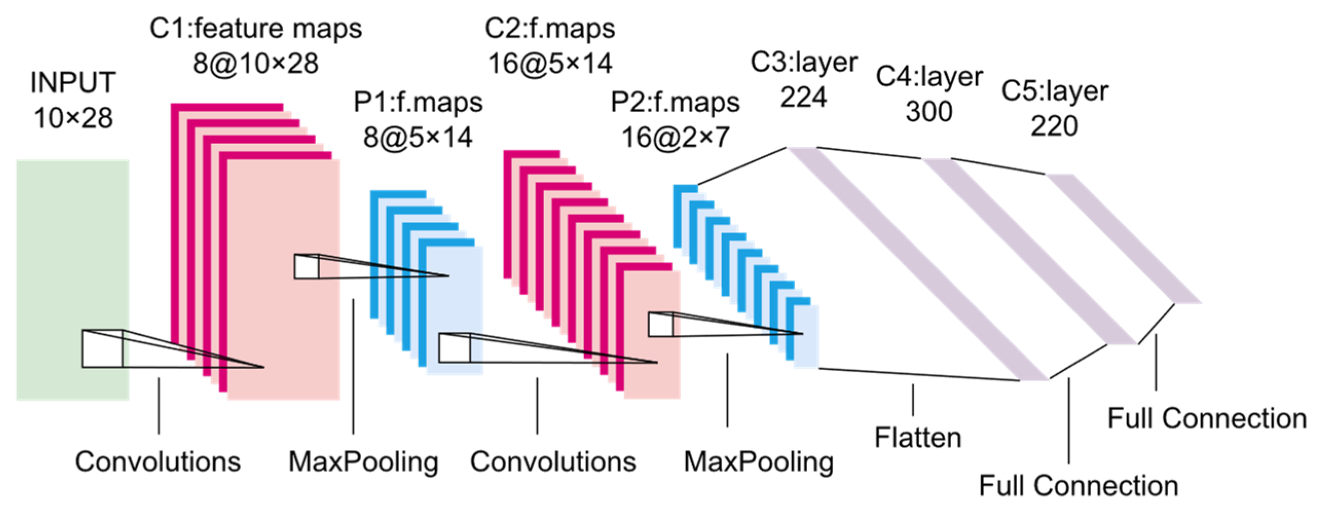
To obtain useful information from historical data while avoiding the use of fully connected networks, which may lead to a large amount of calculation, CNN was applied in this part of the network. The model in this part contained one input layer, two convolutional layers, two pooling layers, two fully connected layers, and one regression output layer. The convolutional and pooling layers were alternately set to form a multi-layer neural network architecture, as shown in Figure 2. The historical atmospheric temperature profiles were inputted to the CNN model, and the features were extracted by it. Then, two dense layers were added for feature fusion after concatenating with the features extracted by MLP. Afterward, the retrieval results combined with historical data and real-time surface parameters were outputted through the last layer.
In order to find the optimal parameters for the proposed network, comparative experiments were conducted to evaluate the performance of the network by varying the number of channels in the output of the first layer of the convolutional layer, the size of the convolutional kernel, and the number of neurons in the fully connected layer. While finding the optimal parameters, the other parameters were kept constant and the performance of the model was compared after 50 training epochs for faster comparison. Based on these evaluations, the depth of the first convolutional layer was chosen as 8, the size of the convolutional kernel was chosen as 2 × 2, and the number of units in the fully connected (FC) layer was chosen as (300,220) as the parameters of the CNN network. The evaluation results are shown in Table 7, Table 8 and Table 9.
After the hyper-optimization of the model, this paper tried to improve the structure of the CNN part and extend the network. The method was to add the same convolutional layers C11 and C22 after the two convolutional layers C1 and C2 and the same FC layers C44 and C55 after the two FC layers C4 and C5 in Figure 3, based on the approach of the VGG (visual geometry group) model, to increase the depth of the network and, thus, improve the inversion results. The improved model structure is shown in Figure 3. The improved temperature profile retrieval model was named the Dense HDTP model.

3.5. Evaluation Methods

The independent validation and test set samples were divided by year and date. To effectively evaluate the model, this study selected three commonly used indicators to assess the inversion effect of the model. Three statistical metrics, namely RMSE, correlation coefficient (R), and mean error (ME), were employed to quantitatively evaluate the retrieval accuracy of the model. The three metrics are as expressed as
R M S E = 1 n i = 1 n ( y i x i ) 2
R = i = 1 n ( x i x ¯ ) ( y i y ¯ ) i = 1 n ( x i x ¯ ) 2 i = 1 n ( y i y ¯ ) 2
M E = 1 n i = 1 n ( y i x i )
where n denotes the number of sample profiles, xi denotes the temperature value of the truth data, and yi denotes the temperature value retrieved by the neural network. x ¯ denotes the average temperature value of the truth data, and y ¯ denotes the average temperature value retrieved by the neural network.

4. Results and Discussion

4.1. Retrieval Results of Method 1 on ERA-5 Data

In the experiment of applying Method 1 to ERA-5 data, 70,128 sets of samples from the data from 1 January 2011 to 31 December 2018 were used to train the network and to establish the inversion model. A total of 17,544 sets of samples from the data from 1 January 2018 to 31 December 2020 were used to optimize the hyperparameters of the network model to verify the accuracy of the model. Finally, 8760 sets of samples from the entire year of 2021 were used to evaluate the generalization ability of the model. 1 set of data represents a predicted temperature profile and a true temperature profile, each profile contains 27 temperature values of pressure levels.
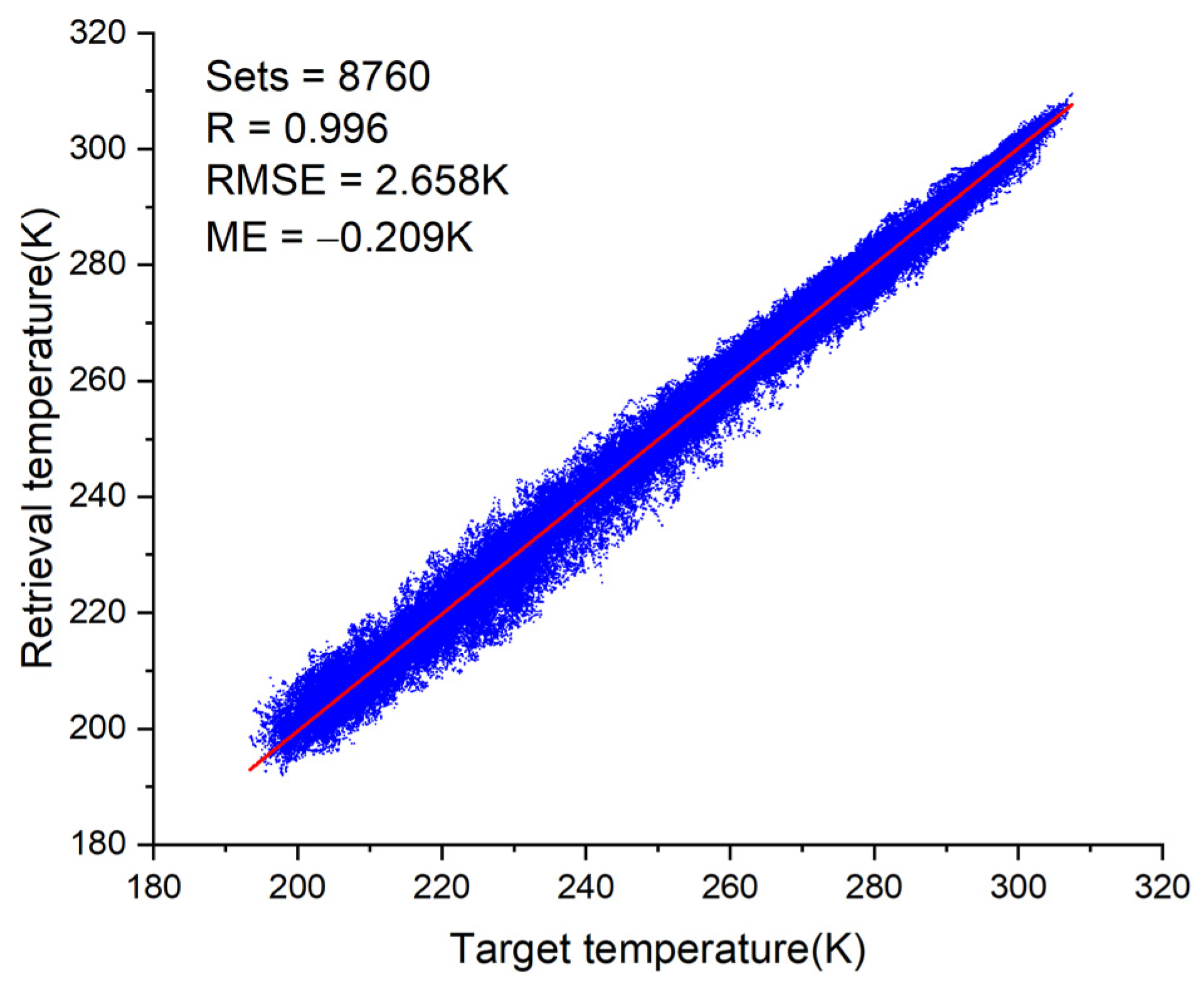
Figure 4 shows a scatter diagram of the retrieved atmospheric temperatures. The number of sets of test samples was 8760, and the vertical pressure ranged from 1000 hPa to 100 hPa with a total of 27 layers. The result showed that the correlation coefficient between the retrieved temperature and the target temperature was 0.996. The RMSE of the atmospheric temperature of the whole layer was 2.658 K, and the ME was −0.209 K.
Figure 5 presents the distribution of the RMSE and ME of the temperature retrieval in this study. As shown in Figure 5a,b, the average RMSE in the troposphere was 2.658 K. The lowest RMSE was observed at 100 hPa, which was 1.544 K; the highest RMSE was observed at 300 hPa, which was 4.113 K. According to the ME distribution, the maximum positive deviation was 0.231 K, and the maximum negative deviation was −0.702 K. The curve was approximately distributed on the negative side of the standard line.
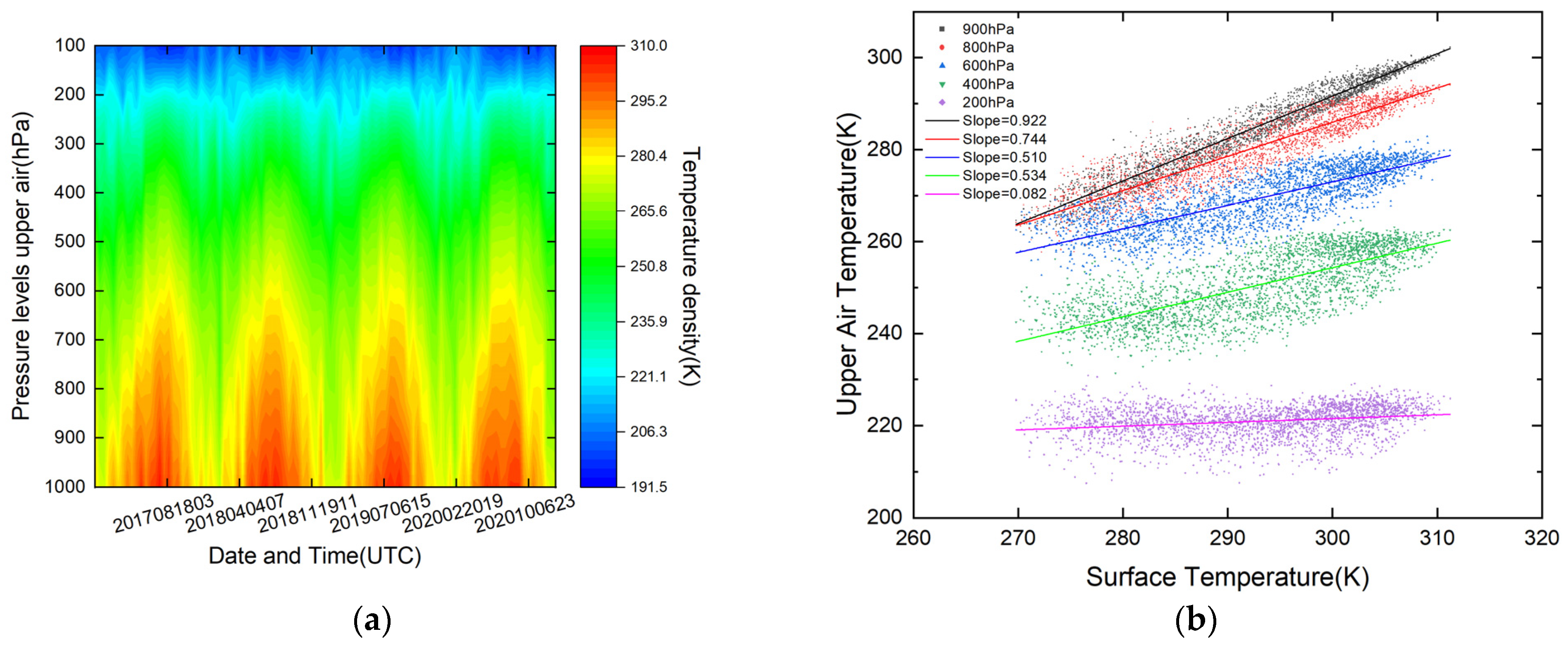
Figure 6a shows the thermal distribution of the ERA-5 reanalysis data and Figure 6b shows the scatter diagram between the upper air temperature at five altitude levels (200, 400, 600, 800, 900 hPa) and surface temperature. The RMSE distribution based on the ERA-5 data increased with altitude and the maximum error occurring around 300 hPa. The atmospheric temperature profiles showed a typical annual periodicity. Temperature profiles near the ground showed an obvious change in the annual cycle. The closer a profile was to the ground, the greater the temperature fluctuation. The further a profile was from the ground, the smaller the temperature fluctuation. Near the top of the troposphere, the vertical rate of temperature change decreased sharply and the temperature of the atmosphere at this point no longer varied seasonally as it did near the surface, in contrast to the base of the troposphere where the temperature was strongly influenced by the surface and the temperature of the atmosphere became less dependent on surface parameters. As shown in Figure 6b, the linear relationship between atmospheric temperature and surface temperature at high altitudes became weaker with increasing altitude. Under the influence of these two factors, the higher the altitude, the greater the atmospheric inversion error.
A comparative experiment was conducted on our model by applying other different parameters, as shown in Table 10. Excluding the surface temperature and surface pressure in Table 10, three surface parameters were adopted as inputs. Table 10 shows the ME and RMSE for different input parameters ranging from small to large in 50 epochs. In terms of performance of mean ME and RMSE, the presence of more input parameters lead to higher accurate inversion results, as Table 10 shows. At present, the mechanism of how wind speed and cloud cover affect the temperature profile was not explored sufficiently, and no obvious linear relationship exists among wind speed and upper-air temperature. However, the absence of these parameters affects the inversion results. Therefore, how to select parameters in actual observation requires further study.

4.2. Retrieval Results of Method 2 on ERA-5 Data

Figure 7 shows a scatter diagram of the retrieved atmospheric temperatures. The dataset was divided on dates in line with the data in Section 4.1. The result showed that the correlation coefficient between the retrieved temperature and the target temperature was 0.997. The RMSE of the atmospheric temperature of the whole layer was 2.265 K, and the ME was −0.256 K.
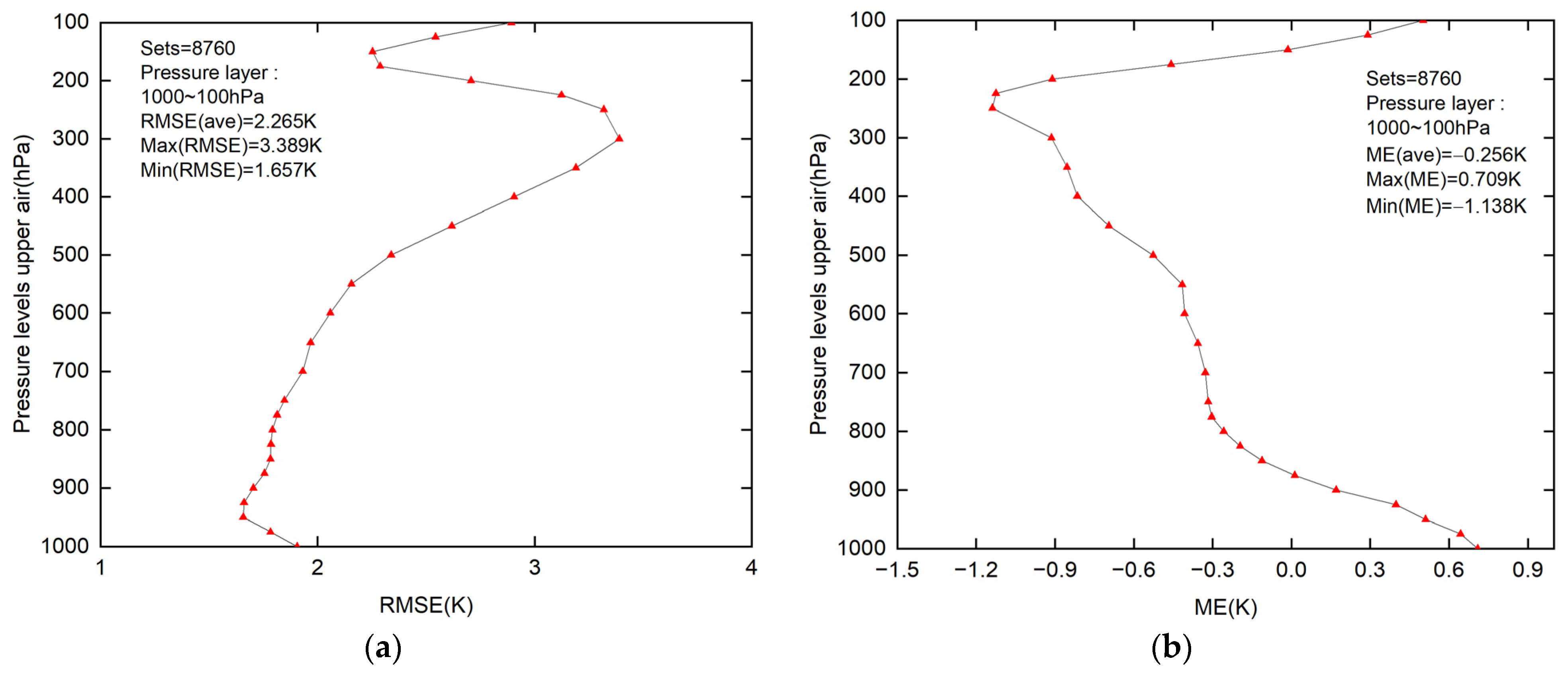
Figure 8 presents the distribution of the RMSE and ME of the temperature retrieval in this study. As shown in Figure 8a,b, the lowest RMSE was observed at 950 hPa, which was 1.657 K; the highest RMSE was observed at 300 hPa, which was 3.389 K. According to the ME distribution, the maximum positive deviation was 0.709 K, and the maximum negative deviation was −1.138 K. The curve was approximately distributed on the negative side of the standard line.

4.3. Comparison between Retrieval Results of Different Methods

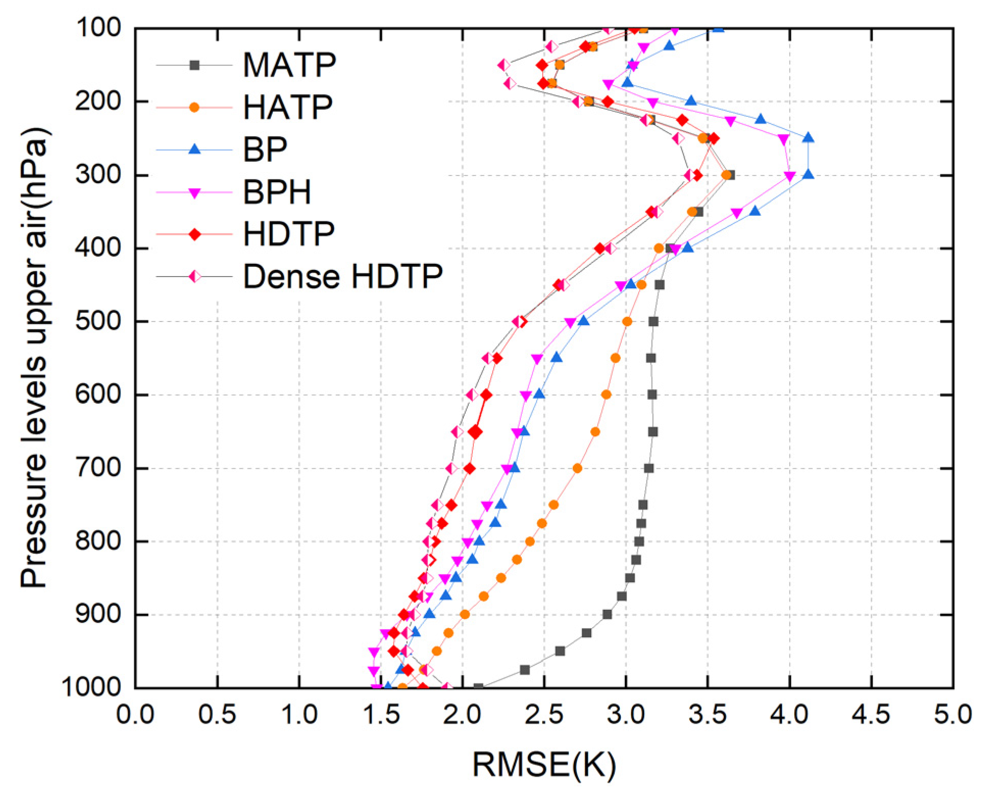
To further evaluate the retrieval results of the proposed method, the temperature profiles obtained from the model were used for further comparisons with the results of other methods by using the same data. With the atmospheric profiles from the ERA-5 data of the validation set samples as the standard profiles, the distribution of RMSE is shown in Figure 9. The method proposed by Qin et al. (2003) [41] is called the monthly average temperature profile (MATP) model in this paper. However, it only included the average temperature profile of each month and did not consider the daily variation. In this work, every monthly average temperature profile was expanded by obtaining the hourly average profiles of this month. This method is called the hourly average temperature profile (HATP) model. The model was based on height values, the analysis in this paper was based on pressure levels, and so, the height values in the equations of the model in the literature [41] were replaced with atmospheric pressure values. This study also performed the inversion of temperature profiles by BP neural networks based on ground observation factors, and this method is also called Method 1 in Section 3.3. Then, the hourly average temperature profiles for the whole year were added to the BP network for training along with the ground surface data as the input parameters. The latter method was called BP Hourly (BPH) to establish a difference from the previous one. As can be observed from Figure 9, the temperature profiles retrieved by the proposed model were the closest to the target data. Compared with the MATP model, the HATP model had more advantages in retrieving the results at a small time scale because the model contained abundant information about the hourly average temperature profile. Figure 9 also indicates that inversion results of BP model were better than those of HATP and MATP models at lower pressure levels of 1000 hPa ~ 400 hPa. However, in the temperature inversion results above 400 hPa, the performance of the BP model was not as good as that of the MATP model. The ground observation parameters were related to the upper-air temperature. Furthermore, the HDTP model proposed in this study included not only the ground observation parameters but also the temperature profile information of the same period in history, and it had the best performance in terms of inversion results. Moreover, due to the use of CNN, the complexity brought by the fully connected network and the loss of the correlation degree of multiple temperature profile data caused by the expansion of the input data into vectors were avoided, so valid information could be extracted from the temperature profile matrix. The inversion results of the Dense HDTP model were better than those of the HDTP model, but the difference was not very significant.

4.4. Retrieval Results Analyzed by Season and Time

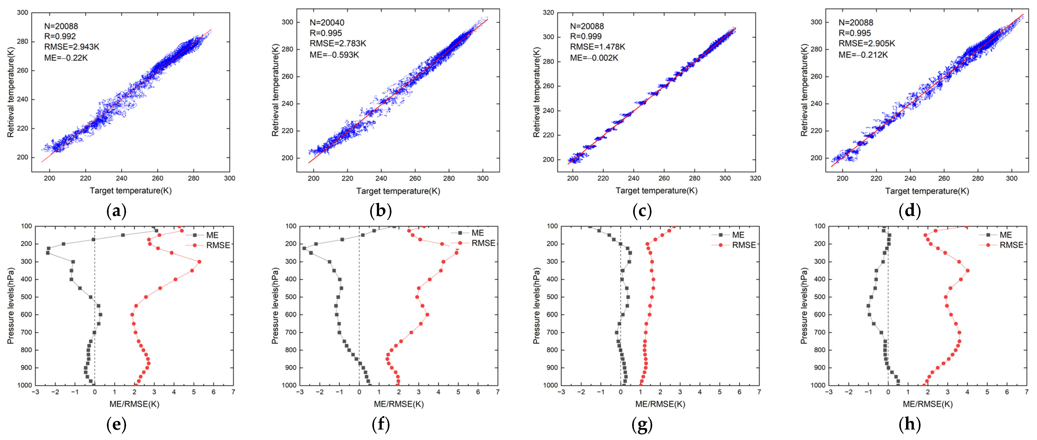
To further evaluate the model, the inversion results were analyzed by different seasons and different times. The inversion results were derived from the HDTP model. The data in January, April, July, and October in 2021 were selected as the representative months of the four seasons, and the inversion results of the mentioned months were compared with the true values. Figure 10a–d show the scatter diagram of the retrieved atmospheric temperature and Figure 10e–h show the distribution of the ME and RMSE of the temperature inversions by pressure levels. From Figure 10, it can be seen that the retrieval results differed in the performance of seasons. The correlation coefficients between the retrieved data and truth data for the above months were 0.992, 0.995, 0.999, 0.995. The ME between the retrieved temperature value and true value were −0.22 K, −0.593 K, −0.002 K, −0.212 K. The RMSE between the retrieved results and target temperature value were 2.934 K, 2.783 K, 1.478 K, 2.905 K. The best performance result occurred in July and the worst performance result occurred in January. The RMSE in January was approximately twice the value of the RMSE in July. From the results of layer-by-layer distribution by pressure, the RMSE value at 300 hPa in January appeared to be the largest throughout the year, and the layer-by-layer RMSE value at 1000 hPa in July appeared to be the smallest. Therefore, the inversion results of this model in summer were evaluated to be the best, and the ME was very small due to the inversion results fluctuating within a small range of the true value. The height of the top of the troposphere depended on the average temperature of the atmosphere; the higher the average temperature, the higher the troposphere was lifted, and the lower the average temperature, the lower the top of the troposphere was. In general, the top of the troposphere in the Chinese land area tends to rise—rise—fall—fall with winter—spring—summer—autumn—winter. The top of the troposphere in each latitude zone had obvious seasonal variations, with the highest in summer and the lowest in winter. As the troposphere rose in summer, the height of the top of the troposphere increased and the relative position of the atmosphere in the troposphere at the same height of 100~400 hPa decreased, thus becoming more seasonally influenced and more closely related to surface temperature. The results show that the smallest RMSE values appeared in July and the most significant change in the RMSE curve between July and other months was the disappearance of the maximum RMSE value at 300 hPa.
The data at 0:00, 6:00, 12:00, and 18:00 UTC in July 2021 were selected as the representative times of the day, and the inversion results of the above times were compared with the true values. Figure 11 shows the scatter diagram of the retrieved atmospheric temperature and the distribution of the ME/RMSE of the temperature inversions by pressure levels. It can be seen from the figure that the inversion results differed in the performance of times. The correlation coefficients between the retrieved data and truth for the above times were all 0.998. The ME between the retrieved temperature value and true value were 0.06 K, 0.018 K, 0.005 K, −0.056 K. The RMSE between the retrieved results and target temperature value were 1.505 K, 1.424 K, 1.457 K, 1.499 K. The best performance result occurred at 6:00 UTC and the worst performance result occurred at 0:00 UTC. The RMSE at 0:00 UTC increased by 5.7% compared to the RMSE at 6:00 UTC. From the results of layer-by-layer distribution by pressure, the layer-by-layer RMSE value at 350 hPa at 0:00 UTC appeared to be the largest throughout the day, and the layer-by-layer RMSE value at 950 hPa at 6:00 UTC appeared to be the smallest. Therefore, the inversion results of this model at 6:00 UTC were evaluated to be the best. The atmospheric temperature profile during the nighttime period was of the nighttime radiation type. As time changed from day to night, the near-surface atmosphere cooled due to radiative cooling. Due to nighttime ground radiative cooling, the near-surface atmospheric temperature increased with increasing height, showing an inversion characteristic, and the inversion error of the temperature profile was large at this time. Therefore, in the early morning period, when the inversion state was strongest, the RMSE of the temperature profile inversion error also reached its maximum. During the day, as the sun’s radiation affected, the ground temperature rose rapidly and broke the inversion distribution of the near-surface layer from the ground to the high altitude. Therefore, the RMSE of the inversion error reached its minimum in the afternoon.

5. Conclusions

In this study, we proposed a method based on historical data and ground observation data to retrieve temperature profiles using neural networks. The neural network can learn the intrinsic relationship between input parameters and inversion parameters. Based on ERA-5 data, we established two machine learning models to invert the atmospheric temperature profile of Fuyang City. The first model directly inverted the atmospheric temperature profile from ground observation data, while the second model inverted the atmospheric temperature profile from ground observation data and historical temperature profile data of the same period. In order to optimize the performance of the model, we conducted experimental confirmation of the hyperparameters for the two models separately and obtained the best performing hyperparameters on the validation set. Finally, the model performed retrieval result verification on hourly temperature profile data for the whole year of 2021 and compared the results of the two models with those of other methods. The results showed that the inversion result of the second model was optimal, and the overall RMSE of the last 27 pressure levels reached 2.265 K.
In order to better evaluate the performance of the inversion model, this paper conducted an error analysis of the layer-by-layer distribution RMSE of the inversion results. Among them, the inversion error near the 300 hPa range was the largest. By analyzing the original data, it can be found that as the height increased, the correlation between high-altitude temperature and ground temperature gradually weakened, and the influence of ground factors on high-altitude temperature became smaller and smaller. Therefore, the result of inverting the temperature profile based on ground parameters was that as the height increased, the inversion error gradually increased. When it reached a height of 300 hPa, the correlation between high-altitude temperature and ground was weakest, and so, the inversion error at this height layer was the largest.
In addition, this paper used the inversion results of January, April, July, and October 2021 to represent the inversion performance of temperature profiles in spring, summer, autumn and winter, respectively. The results showed that the inversion result in July was the best with an RMSE of 1.478 K, while the inversion result in January was the worst with an RMSE of 2.934 K. Afterwards, we analyzed the reasons for the difference in inversion results by combining the distribution characteristics of atmospheric temperature profiles with the seasonal changes of the troposphere. This paper used the inversion results at 0:00 (UTC), 06:00 (UTC), 12:00 (UTC), and 18:00 (UTC) in July 2021 to evaluate the inversion performance of temperature profiles at different times. The results showed that the inversion result at 06:00 (UTC) was the best with an RMSE of 1.424 K, while the inversion result at 0:00 (UTC) was the worst with an RMSE of 1.505 K. Afterwards, we explained the error pattern of temperature profile inversion by combining the atmospheric structure and change rules of the boundary layer.
The proposed model achieved some success in the research of inverting atmospheric temperature profiles. Using the method proposed in this paper, it is easy to obtain data and it is simple in principle, but the current accuracy is not high enough and there is still a certain gap in the inversion accuracy of temperature profiles obtained by traditional detection and remote sensing methods. In the future, in order to improve the accuracy of temperature profile inversion using machine learning methods, we will consider adding more observation parameters to achieve the improvement of inversion accuracy.

Author Contributions

H.W. designed the temperature retrieval model; D.L. prepared and provided the temperature data of ground-based observation; D.L., Y.X., Y.W. and W.X. provided useful suggestions for the experiment and support for the writing; H.W. prepared the article with contributions from all the coauthors. All authors have read and agreed to the published version of the manuscript.

Funding

This research was supported by Key Collaborative Research Program of the Alliance of International Science Organizations (Grant No. ANSO-CR-KP-2020-09), the Research on Key Technologies of Airport Nowcasting Cloud Height Detection System Based on Vision and Laser Collaboration (202104b11020028), and the Research on Development and Demonstration Application of Marine Multi-band Cloud and Fog Observation Equipment (2021YFC3090200).

Data Availability Statement

Not applicable.

Conflicts of Interest

The authors declare no conflict of interest.

References

  1. Wang, Y.; Huang, Y.; Huang, S.Y. A preliminary study of the retrieval methods for atmosphere and humidity profiles. Remote Sens. Land Resour. 2008, 27, 23–26. [Google Scholar] [CrossRef]
  2. Cao, X.F.; Li, X.Y.; Luo, Q.; Liu, S.H.; Li, P.; Liu, X. Review of temperature profile inversion of satellite-borne infrared hyperspectral sensors. Natl. Remote Sens. Bull. 2021, 25, 577–598. [Google Scholar] [CrossRef]
  3. Tan, M.; Wang, B.X.; Zhuang, P.; Zhang, Z.Y.; Li, L.; Chu, Y.F.; Xie, C.B.; Wang, Y.J. Study on Atmospheric Temperature and Water-Vapor Mixing Ratio Based on Raman Lidar. Spectrosc. Spectr. Anal. 2020, 40, 1397. [Google Scholar] [CrossRef]
  4. Dong, C.H.; Li, J.; Zhang, P. Principle and Application of Hyperspectral Infrared Remote Sensing of Atmosphere; Beijing Science Press: Beijing, China, 2013. [Google Scholar]
  5. Bao, Y.S.; Wang, Z.J.; Chen, Q.; Zhou, A.M.; Dong, Y.H.; Min, J.Z. Preliminary Study on Atmospheric Temperature Profiles Retrieval from GIIRS Based on FY-4A Satellite. Aerosp. Shanghai 2017, 34, 28–37. [Google Scholar] [CrossRef]
  6. Luo, S.; Yin, Q. Statistical characteristics analysis of global temperature vertical profile. J. Trop. Meteorol. 2019, 35, 556–566. [Google Scholar] [CrossRef]
  7. Clough, S.A.; Iancono, M.J.; Moncet, J.L. Line-by-line calculation of atmospheric fluxes and cooling rates: Application to water vapour. J. Geophys. Res. Atmos. 1992, 97, 15761–15785. [Google Scholar] [CrossRef]
  8. Isaacs, R.G.; Wang, W.C.; Worsham, R.D.; Goldenberg, S. Multiple scattering LOWTRAN and FASCODE models. Appl. Opt. 1987, 26, 1272–1281. [Google Scholar] [CrossRef] [PubMed]
  9. Kneizys, F.X.; Shettle, E.P.; Abreu, L.W.; Chetwynd, J.H.; Anderson, G.P.; Gallery, W.O.; Selby, J.E.A.; Clough, S.A. Users Guide to LOWTRAN 7, AFGL-TR-88-0177. 1988. Available online: https://apps.dtic.mil/dtic/tr/fulltext/u2/a206773.pdf (accessed on 28 November 2020).
  10. Berk, A.; Anderson, G.P.; Acharya, P.K. MODTRAN4 USER’S MANUAL; Technical Report: Hanscom AFB, MA, USA, 2002. [Google Scholar]
  11. Wang, P.; Liu, K.Y.; Cwik, T.; Green, R. MODTRAN on supercomputers and parallel computers. Parallel Comput. 2002, 28, 53–64. [Google Scholar] [CrossRef]
  12. Anderson, G.P.; Clough, S.A.; Kneizys, F.X.; Chetwynd, J.H.; Shettle, E.P. AFGL Atmospheric Constituent Profiles; Environmental Research Papers; AFGL-TR-89-0110; Air Force Geophysics Laboratory: Bedford, MA, USA, 1986; Volume 954. [Google Scholar]
  13. Wei, H.L.; Chen, X.H.; Rao, R.Z. Introduction to the Combined Atmospheric Radiative Transfer Software CART. J. Atmos. Environ. Opt. 2007, 2, 446–450. [Google Scholar] [CrossRef]
  14. Chen, X.H.; Wei, H.L. Variation of Infrared Atmospheric Transmittance Based on Atmospheric Models in Typical Regions of China. Laser Infrared 2008, 38, 1090–1093. [Google Scholar] [CrossRef]
  15. Qi, C.H.; Liu, H.; Ma, G.; Zhang, P.; Wu, X.B. A Sampling Technique of Typical Atmospheric Profiles Database in China. J. Appl. Meteorol. Sci. 2010, 21, 70–75. [Google Scholar] [CrossRef]
  16. Huang, J. The Study on the Algorithm of Retrieving the Temperature and Moisture Profile from Satellite Infrared Measurements. Master’s Thesis, Lanzhou University, Gansu, China, 2006. [Google Scholar]
  17. Lv, D.R.; Wang, P.C.; Jinhuan, Q.; Tao, S.Y. An Overview on the Research Progress of Atmospheric Remote Sensing and Satellite Meteorology in China. Chin. J. Atmos. Sci. 2003, 27, 552–566. [Google Scholar] [CrossRef]
  18. Huang, W.; Gao, T.C.; Liu, L. Review of Remote Sensing Retrieval of Temperature and Water Vapor Profiles Using Ground-based Infrared Hyper-spectral Data. Infrared 2015, 36, 1–6. [Google Scholar] [CrossRef]
  19. Wang, Z.C.; Zhang, X.F.; Mao, J.J.; Ji, C.L. Overview of ground-based remote sensing observation techniques for air temperature, humidity and wind profiles. Meteorol. Hydrol. Mar. Instrum. 2018, 35, 109–116. [Google Scholar] [CrossRef]
  20. Yin, Q.; He, J.H.; Zhang, H. Application of laser radar in monitoring meteorological and atmospheric environment. Weather. Environ. 2009, 25, 48–56. [Google Scholar] [CrossRef]
  21. Liu, S.B.; He, W.Y.; Liu, H.Y.; Chen, H.B. Retrieval of atmospheric boundary layer height from ground-based microwave radiometer measurements. J. Appl. Meteorol. Sci. 2015, 26, 626–635. [Google Scholar] [CrossRef]
  22. Li, S.C.; Wang, D.L.; Li, Q.M.; Song, Y.H.; Liu, L.J.; Hua, D.X. Pure rotational Raman lidar for absolute detection of atmospheric temperature. Acta Phys. Sin. 2016, 65, 143301. [Google Scholar] [CrossRef]
  23. Shang, Z.; Xie, C.B.; Wang, B.X.; Tan, M.; Zhong, Z.Q.; Wang, Z.Z.; Liu, D.; Wang, Y.J. Pure rotational Raman lidar measurements of atmospheric temperature near ground in Beijing. Infrared Laser Eng. 2017, 46, 119–126. [Google Scholar]
  24. Cooney, J. Measurement of atmospheric temperature profiles by Raman backscatter. J. Appl. Meteorol. 1972, 11, 108–112. [Google Scholar] [CrossRef]
  25. Huang, X.Y.; Zhang, X.; Leng, L.; Li, F.; Fan, Y.W. Study on retrieval methods with MonoRTM for microwave radiometer measurements. J. Meteorol. Sci. 2013, 33, 138–145. [Google Scholar] [CrossRef]
  26. Mao, J.T.; Zheng, G.G. Discussions on some weather modification issues. J. Appl. Meteorol. Sci. 2006, 17, 643–646. [Google Scholar] [CrossRef]
  27. Kang, X.Y.; Zhang, B.Y.; Tian, J.B.; Liu, N.; Ma, X.Q. Applicability of Products Rretrieved from Microwave Radiometer in East Qinghai Province. Arid Zone Res. 2019, 36, 356–364. [Google Scholar] [CrossRef]
  28. Li, N.; Zhang, W.; Chen, Y.; Liu, D.; Shi, J.S.; Zhang, B.D. Remote-sensing of atmospheric temperature and relative humidity profiles based on microwave radiometer. J. Lanzhou Univ. 2015, 51, 61–71. [Google Scholar] [CrossRef]
  29. Tian, J.B.; Zhang, Y.X.; Yan, H.Q.; Tang, W.T.; Kang, X.Y. Study on Neural Network Algorithm for Retrieving Atmospheric Profile Based on Microwave Radiometer in Plateau Region. Plateau Mt. Meteorol. Res. 2021, 41, 125–134. [Google Scholar] [CrossRef]
  30. Bao, Y.S.; Cai, X.; Qian, C.; Min, J.Z.; Lu, Q.F.; Zuo, Q. 0–10 km temperature and humidity profiles retrieval from ground-based microwave radiometer. J. Trop. Meteorol. 2018, 24, 243–252. [Google Scholar] [CrossRef]
  31. Cai, X.; Bao, Y.S.; Petropoulos, G.P.; Liu, F.; Lu, Q.F.; Zhu, L.H.; Wu, Y. Temperature and Humidity Profile Retrieval from FY4-GIIRS Hyperspectral Data Using Artificial Neural Networks. Remote Sens. 2020, 12, 1872. [Google Scholar] [CrossRef]
  32. Wang, G.; Chen, J.; Dai, J.; Wang, Y. Bias Correction of Brightness Temperatures in Medium Wave Channel of FY-4A Infrared Hyperspectral GIIRS. Infrared 2021, 42, 39–44. [Google Scholar] [CrossRef]
  33. Yao, S.H.; Guan, L. Atmospheric temperature and humidity profile retrievals using a machine learning algorithm based on satellite-based infrared hyperspectral observations. Infrared Laser Eng. 2022, 51, 20210707. [Google Scholar] [CrossRef]
  34. Huang, P.; Guo, Q.; Han, C.; Tu, H.; Zhang, C.; Yang, T.; Huang, S. An Improved Method Combining CNN and 1D-Var for the Retrieval of Atmospheric Humidity Profiles from FY-4A/GIIRS Hyperspectral Data. Remote Sens. 2021, 13, 4737. [Google Scholar] [CrossRef]
  35. Guan, Y.H.; Ren, J.; Bao, Y.S.; Lu, Q.F.; Liu, H.; Xiao, X.J. Research of the infrared high spectral (IASI) satellite remote sensing atmospheric temperature and humidity profiles based on the one-dimensional variational algorithm. Trans. Atmos. Sci. 2019, 42, 602–611. [Google Scholar] [CrossRef]
  36. Zhen-xiang, S.H.E.N.; Chao-shun, L.I.U. A study on the inversion of atmospheric temperature and humidity profiles by using CrIS infrared hyperspectral satellite data. J. East China Norm. Univ. (Nat. Sci.) 2019, 205, 199–210. [Google Scholar] [CrossRef]
  37. Guan, L.; Zhang, X.H.; Liu, Y. Application of Artificial Neural Network Algorithm in Retrieving Atmospheric Temperature Profiles from Hyperspectral Infrared Data. Trans. Atmos. Sci. 2010, 33, 341–346. [Google Scholar] [CrossRef]
  38. Milstein, A.B.; Blackwell, W.J. Neural network temperature and moisture retrieval algorithm validation for AIRS/AMSU and CrIS/ATMS. J. Geophys. Res. Atmos. 2016, 121, 1414–1430. [Google Scholar] [CrossRef]
  39. Mahngren-Hansen, D.; Laparra, V.; Nielsen, A.A.; Camps-Valls, G. Statistical retrieval of atmospheric profiles with deep convolutional neural networks. ISPRS J. Photogramm. Remote Sens. 2019, 158, 231–240. [Google Scholar] [CrossRef]
  40. Han, J.; Guan, L.; Wang, Z.H.; Zhang, X.H. The Influence of Surface Temperature on the Retrieval of Clear-sky Air Temperature Vertical Profile. Atmos. Sci. Res. Appl. 2009, 36, 81–86. [Google Scholar]
  41. QIN, Q.B.; Wei, H.L. Construction of Real-Time Atmospheric Parameter Profiles Based on the Average Radiosonde Profiles and the Surface Meteological Datas. J. Atmos. Environ. Opt. 2013, 8, 161–168. [Google Scholar] [CrossRef]
  42. Bauer, P.; Thorpe, A.; Brunet, G. The quiet revolution of numerical weather prediction. Nature 2015, 525, 47–55. [Google Scholar] [CrossRef] [PubMed]
  43. Hersbach, H.; Bell, B.; Berrisford, P.; Hirahara, S.; Horanyi, A.; Munoz-Sabater, J.; Nicolas, J.; Peubey, C.; Radu, R.; Schepers, D. The ERA5 global reanalysis. Q. J. R. Meteorol. Soc. 2020, 146, 1999–2049. [Google Scholar] [CrossRef]
  44. Meng, X.G.; Guo, J.J.; Han, Y.Q. Preliminarily assessment of ERA5 reanalysis data. J. Mar. Meteorol. 2018, 38, 91–99. [Google Scholar] [CrossRef]
  45. Hoffmann, L.; Günther, G.; Li, D.; Stein, O.; Wu, X.; Griessbach, S.; Heng, Y.; Konopka, P.; Müller, R.; Vogel, B.; et al. From ERA-Interim to ERA5: The considerable impact of ECMWF’s next-generation reanalysis on Lagrangian transport simulations. Atmos. Chem. Phys. 2019, 19, 3097–3124. [Google Scholar] [CrossRef]
  46. Liu, T.T.; Zhu, X.F.; Guo, R.; Xu, K.; Zhang, S.Z. Applicability of ERA5 reanalysis of precipitation data in China. Arid Land Geogr. 2022, 45, 66–79. [Google Scholar] [CrossRef]
  47. Davis, D.T.; Chen, Z.; Tsang, L.; Hwang, J.-N.; Chang, A.T.C. Retrieval of snow parameters by iterative inversion of a neural network. IEEE Trans. Geosci. Remote Sens. 1993, 31, 842–852. [Google Scholar] [CrossRef]
  48. Jin, Y.Q.; Liu, C. Biomass retrieval from high-dimensional active/passive remote sensing data by using artificial neural networks. Int. J. Remote Sens. 1997, 18, 971–979. [Google Scholar] [CrossRef]
  49. Blackwell, W.J. A neural-network technique for the retrieval of atmospheric temperature and moisture profiles from high spectral resolution sounding data. IEEE Trans. Geosci. Remote Sens. 2005, 43, 2535–2546. [Google Scholar] [CrossRef]
  50. Mao, K.S.; Shi, J.; Tang, H.; Guo, Y.; Qiu, Y.; Li, L. A neural-network technique for retrieving land surface temperature from AMSR-E passive microwave data. In Proceedings of the 2007 IEEE International Geoscience and Remote Sensing Symposium, Barcelona, Spain, 23–28 July 2007; pp. 4422–4425. [Google Scholar] [CrossRef]
  51. Cong, S.; Wei, X. Design and Selection of Construction, Parameters and Training Method of BP Network. Comput. Eng. 2001, 27, 3. [Google Scholar] [CrossRef]
  52. Rikiya, Y.; Mizuho, N.; Gian, D.K.R.; Kaori, T. Convolutional neural networks: An overview and application in radiology. Insights Into Imaging 2018, 9, 611–629. [Google Scholar] [CrossRef]
  53. Lu, H.T.; Zhang, Q.C. Applications of Deep Convolutional Neural Network in Computer Vision. J. Data Acquis. Process. 2016, 31, 1–17. [Google Scholar] [CrossRef]
  54. Zhou, H.Q.; Huang, L.L.; Wang, Y.T. Deep learning algorithm and its application in optics. Infrared Laser Eng. 2019, 48, 229–318. [Google Scholar] [CrossRef]
  55. Li, H.; Zhe, L.; Shen, X.; Brandt, J.; Gang, H. A convolutional neural network cascade for face detection. In Proceedings of the 2015 IEEE Conference on Computer Vision and Pattern Recognition (CVPR), Boston, MA, USA, 7–12 June 2015; pp. 5325–5334. [Google Scholar] [CrossRef]
  56. Huang, Z.; Ming, D.; Mao, Q.; Zhan, Y. Speech Emotion Recognition Using CNN. In Proceedings of the ACM International Conference, Orlando, FL, USA, 3–7 November 2014; pp. 801–804. [Google Scholar] [CrossRef]
Figure 1. Overall structure of the HDTP model.
Remotesensing 15 02717 g001
Figure 2. CNN architecture.
Remotesensing 15 02717 g002
Figure 3. CNN architecture with VGG model approach.
Remotesensing 15 02717 g003
Figure 4. Scatter diagram of temperature retrieval results of Method 1 on ERA-5 data.
Remotesensing 15 02717 g004
Figure 5. RMSE and ME distribution of the retrieval temperature on different pressure levels: (a) RMSE distribution map for temperature on pressure levels; (b) ME distribution map for temperature on pressure levels.
Remotesensing 15 02717 g005
Figure 6. Atmospheric temperature profile distribution: (a) Atmospheric temperature profile time series from 1 January 2017 to 31 December 2020; (b) scatter diagram between the temperature at five altitude levels (200, 400, 600, 800, 900 hPa) and surface temperature.
Remotesensing 15 02717 g006
Figure 7. Scatter diagram of temperature retrieval results of the Dense HDTP model.
Remotesensing 15 02717 g007
Figure 8. RMSE and ME distribution of the retrieval temperature on different pressure levels: (a) RMSE distribution map; (b) ME distribution map.
Remotesensing 15 02717 g008
Figure 9. Comparison of the retrieval results of different methods and our model: RMSE for temperature on pressure levels.
Remotesensing 15 02717 g009
Figure 10. Scatter diagram of the retrieved atmospheric temperature and the ME/RMSE of the temperature inversions by pressure levels: (ad) scatter diagram of temperature retrieval in January, April, July, and October in 2021; (eh) ME/RMSE for temperature on pressure levels in January, April, July, and October in 2021.
Remotesensing 15 02717 g010
Figure 11. Scatter diagram of the retrieved atmospheric temperature and the ME/RMSE of the temperature inversions by pressure levels: (ad) scatter diagram of temperature retrieval at 0:00, 6:00, 12:00, and 18:00 UTC in July 2021; (eh) ME/RMSE for temperature on pressure levels at 0:00, 6:00, 12:00, and 18:00 UTC in July 2021.
Remotesensing 15 02717 g011
Table 1. Description of the ERA-5 data in the study.
Data TypeGridded
ProjectionRegular latitude–longitude grid
Horizontal coverage(32°N–33°N, 115°E–116°E)
Horizontal resolution0.25° × 0.25°
Vertical coverage1000 hPa to 100 hPa
Vertical resolution27 pressure levels
Temporal coverage2001 to 2021
Table 2. Main variables of the ERA-5 surface data in the study.
NameUnits
2 m temperatureK
2 m dewpoint temperatureK
Surface pressurePa
10 m u-component of windm/s
10 m v-component of windm/s
Total cloud coverDimensionless
Table 3. Main input and output parameters of Method 1 using ERA-5 data.
Input ParametersOutput Parameters
Month day hourTemperature at 1000 hPa
2 m temperatureTemperature at 975 hPa
2 m dewpoint temperatureTemperature at 950 hPa
Surface pressure……
10 m u-component of windTemperature at 150 hPa
10 m v-component of windTemperature at 125 hPa
Total cloud coverTemperature at 100 hPa
Table 4. Main input1 and output parameters of Method 2 using ERA-5 data.
Input1 ParametersOutput Parameters
Month day hourTemperature at 1000 hPa
2 m temperatureTemperature at 975 hPa
2 m dewpoint temperatureTemperature at 950 hPa
Surface pressure……
10 m u-component of windTemperature at 150 hPa
10 m v-component of windTemperature at 125 hPa
Total cloud coverTemperature at 100 hPa
Table 5. Main input2 parameters of Method 2 using ERA-5 data.
Input2 Parameters
Y10Y9……Y2Y1
T0T0……T0T0
T1000T1000……T1000T1000
T975T975……T975T975
…………………………
T125T125……T125T125
T100T100……T100T100
Table 6. Performance of the BP network on ERA-5 data with varying units in the hidden layers in 50 epochs.
Units1Units2Validation RMSE (K)Training Time (min)
2603002.7450.51
3003002.7220.51
3403002.7420.52
3002602.6890.52
3002202.7270.52
Table 7. Performance of the CNN on ERA-5 data with varying depths of C1 in 50 epochs, size of kernels in convolutional layers is 3 × 3 and number of units in FC layers is (300,300).
Depth of C1Validation RMSE (K)Training Time (min)
42.6921.27
82.6231.34
162.6441.44
322.6831.80
Table 8. Performance of the CNN on ERA-5 data with varying size of kernels in convolutional layers in 50 epochs, the depth of C1 is 8 and number of units in FC layers is (300,300).
Kernel SizeValidation RMSE (K)Training Time (min)
2 × 22.5921.32
3 × 32.6271.34
4 × 42.6541.34
5 × 52.6921.35
Table 9. Performance of the CNN on ERA-5 data with varying number of units in FC layers in 50 epochs, the depth of C1 is 8 and size of kernels in convolutional layers is 2 × 2.
FC Layer 1FC Layer 2Validation RMSE (K)Training Time (min)
3003002.5921.32
3002602.5631.32
3002202.5521.29
3002002.5831.31
2602202.5841.32
2202202.5941.32
2002202.6031.32
Table 10. Comparison of the ME and RMSE between different input parameters (in 50 epochs).
No.12345678
2 m dewpoint temperature----
10 m wind----
Total cloud cover----
ME−0.278−0.220−0.368−0.350−0.286−0.137−0.282−0.261
RMSE2.9662.8302.8552.8772.7352.8772.7242.637
Disclaimer/Publisher’s Note: The statements, opinions and data contained in all publications are solely those of the individual author(s) and contributor(s) and not of MDPI and/or the editor(s). MDPI and/or the editor(s) disclaim responsibility for any injury to people or property resulting from any ideas, methods, instructions or products referred to in the content.