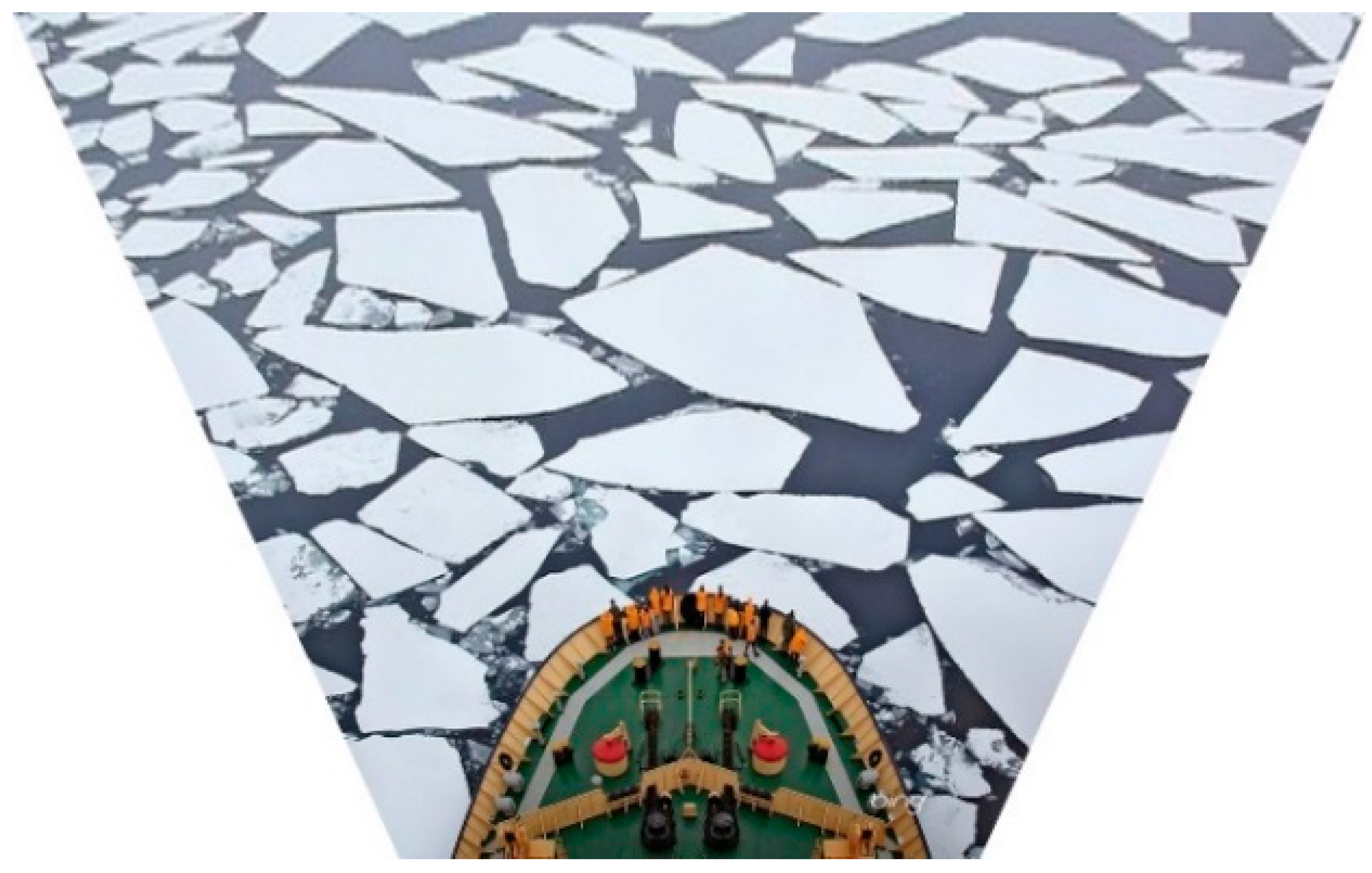
1. Introduction
With the increasing exploration and exploitation of hydrocarbons in ice-covered waters, more attention is being paid to marine operations impacted by ice [
1]. The greatest challenge to Arctic navigation is sea ice, which covers approximately 7% of the world’s oceans [
2]. Sea ice concentration and floe size distribution are the key parameters that significantly impact navigability. In cold regions, sea ice comes in various sizes, ranging from meters to kilometers in size, and an icebreaker traveling through an area of high sea ice concentration or large floe size must consider whether the ice conditions can support safe passage. Therefore, real-time monitoring and an identification of the size and shape of floes contribute to automatically detecting hazardous conditions [
3,
4] and the auxiliary decision making for ship navigation in cold regions. Additionally, this floe size distribution is crucial in forming a digital ice field. In numerical simulations of ice loads in a broken ice field [
5,
6,
7,
8,
9,
10,
11], the floe size distribution in the digital ice field is approximately estimated based on the ice tank test. If computer vision is used to measure the actual floe size distribution of the broken ice field, the accuracy of the numerical simulations will improve.
However, the retrieval of sea ice information from observational data sets is still limited due to noise from the complex polar environment and a lack of efficient equipment and algorithms for processing cold region images. Therefore, the development of technology for high-resolution field observations and estimations of ice floe size distribution is necessary and meaningful.
Using optical images taken by ship-based cameras is one of the best ways to observe the sea ice conditions in cold regions. Digital image processing techniques can reduce uncertainties in the environment and suppress errors regarding objects, obtaining more reliable information on the sea ice conditions [
12]. In ice-covered regions, cameras are commonly used as sensors to characterize these ice conditions [
13,
14]. Ship-based observations and remote sensing are currently the main methods used to obtain images of ice-covered regions. Lu and Li [
15] attached cameras to a ship to take photos and obtain the ice concentration and floe size. Zhang and Skjetne [
16] installed cameras on an unmanned aerial vehicle (UAV) to collect data on sea ice and measure the ice statistics and properties.
Remote sensing is a crucial tool used in polar sea ice research [
17,
18,
19]. Synthetic-aperture radar (SAR) imaging plays an essential role in sea ice data analysis, as it is not restricted by environmental factors, enabling the data to be continuously collected in all weather conditions and through the polar night [
20]. However, using satellite high-resolution optical instruments incurs high application costs and cannot distinguish open water from pond ice and persistent cloud cover [
21]. To address this, Yan et al. [
22] used convolutional neural networks (CNN) to extract the sea ice concentration from Global Navigation Satellite Signal Reflectometry (GNSS-R) data and Zhu et al. [
23] used machine learning to classify sea ice with GNSS-R data. Meanwhile, sea ice photography conducted with digital cameras is widely used to determine the actual ice conditions encountered by a ship or aircraft [
24,
25]. Optical sensors are not suitable for use in the dark and harsh weather; however, shipborne photography is cost-effective, automated, and easy to operate, making it a common method used for scientific expeditions in the polar regions.
When retrieving ice statistics from obtained images, the method of digital image processing determines the quality of the ice information. In an actual ice-covered environment, ice floes usually touch each other closely, making it challenging to identify their borders from optical images. Several researchers have tried to mitigate this issue through a boundary detection of the individual ice floes and an ice floe analysis [
16,
17,
26]. Extracting these ice floes from images is also a significant challenge. Zhang et al. [
26] used threshold segmentation to divide the image into “object area” and “background area,” which could identify the sea ice. However, the threshold needs to be adjusted when processing images captured in different light conditions [
27] and the illumination affects the result. There are many deep learning methods that can be used to identify sea ice, such as YOLO proposed by Redmon et al. [
28], which can automatically identify the class and location information of ice. YOLACT, proposed by Bolya et al. [
29], is a deep convolutional neural network and can recognize different classes at the pixel level.
To calculate the sea ice concentration of the bow area, images captured by a camera in an outward-looking orientation are used. These images typically contain sea ice, water, and ships, making it necessary to distinguish between these three objects and extract the ice. To accomplish this, sea ice images are collected and used to create a dataset for training the YOLACT network. The trained instance segmentation model can distinguish the sea ice and remove the water and ships from the images. Once the mask of sea ice has been extracted, the number of sea ice pixels can be calculated. The real area of the sea ice is proportional to the number of pixels, which can be calculated according to the ratio between the pixel distance and the actual distance. With the acquisition of the real area, the floe size distribution and ice concentration can be calculated from the resulting data.
2. Description of YOLACT Network
First, we utilize the YOLACT network to calculate the sea ice concentration, drawing on previous knowledge of the network and our observations of the sea ice. Next, we detail the construction of the dataset used for the sea ice identification, as well as the process of the model training and testing. Finally, we explain the method used for calculating the ice concentration.
2.1. Model Description
The YOLACT network, proposed by Bolya et al. [
29], is an instance segmentation network. Unlike other methods of sea ice identification, YOLACT is a deep learning method that can identify multiple objects in a complex environment. It can detect images taken in different lighting conditions and identify objects other than sea ice.
Figure 1 illustrates the YOLACT network, which, similar to other networks, utilizes the multi-scale feature map and Feature Pyramid Network (FPN) technique proposed by Zhao et al. [
30]. The backbone extracts features and transfers feature information to the prediction network through the feature pyramid. The network divides complex detection tasks into two parallel processes to speed up the detection. One branch uses ProtoNet to generate a prototype mask and the other approach uses the prediction header to process the position and show the coefficients, which are filtered by the NMS. In this paper, we adjust the NMS in the network to fit the task of sea ice identification, as the common parameters of NMS can lead to missed detections when detecting images with a high sea ice concentration. The obtained result is linearly combined with the original mask to yield the segmentation of each instance.
2.2. Dataset for Training Model
To ensure that the trained model can be applied to different environments, it is important not only to select a suitable model, but also to choose images captured in various situations as datasets, such as model ice in an ice tank, sea ice in open water, and images containing both ice breakers and ice in one picture.
The images of the model ice were obtained from the multifunctional ice basin of the Marine Technology Group at Aalto University. The camera captured the model ice images, which usually covered a large area, from the passage above the ice basin. To enhance the applicability of the trained model, we varied the illumination conditions and shooting angles of the camera, as shown in
Figure 2. This diversified the dataset to include various detection scenarios, making the trained model suitable for images captured not only from a suitable illumination environment, but also from complex environments and even open water.
During the model testing, we were not required to obtain the ice concentration for the entire ice basin, as this is typically limited to a small area of interest, such as the ice–structure interaction region near the bow. Globally extracting a segmentation of the model ice and background from a whole ice basin image may cause the loss of some ice information, especially when an image suffers from non-uniform illumination or shadow problems. Moreover, sea ice images usually contain multiple ice floes that are closely connected, as shown in
Figure 2a, and some parts of floe boundaries can become weaker than others. This problem becomes more challenging with an increasing picture-shooting range. Decreasing the shooting range, however, can result in a loss of information, reducing the amount of valid data for the training set and slowing down the model convergence speed. Moreover, it can enhance noise and affect the segmentation for the detection set. Therefore, we needed to ensure that the images contained sufficient information for creating a good training set and adjust the parameters during the training to minimize the information loss. To make the trained model better suited for sea ice detection, we also included some images of crushing ice fields in the dataset, as illustrated in
Figure 3.
To classify the ice, ice breakers, and water in the images, the samples were grouped into two classes: ice and ship, while the water was considered as the background of the image. The purpose of this classification was to determine whether the trained model could differentiate the sea ice and ice breakers from the water, which would enable the mapping of the quantitative sea ice concentration. During all the tests, 80% of the dataset was allocated for training and 20% for validation.
2.3. Model Training and Testing
In this experiment, the YOLACT model used the ResNet50 network and was trained for 40,000 iterations with an initial learning rate of 0.01. The decay was set to occur at the 20,000th, 30,000th, and 35,000th iterations, respectively, with a decay rate of 10% of the current learning rate. Additionally, because the images of the sea ice were taken from high angles, the image size was enhanced to 1000 (normally set to 500). The “image size” parameter refers to the size of the input image into the neural network. The actual size of the images taken from the ice basin could be up to 1200 and the large shooting range captured a significant amount of sea ice. If we continued to set the image size to 550, the small size of ice blocks in the images may not have been clear enough to train the model. For the instance segmentation of sea ice, the main evaluation metric used was average precision (
AP). To determine whether an object was accurately segmented, the Intersection over Union (IoU) threshold could be used to express the similarity coefficient between the two sets of data. In instance segmentation, IoU represents the overlap area between the predicted sea ice mask
Mp and the real sea ice mask
MGT, divided by the union area between them, as follows:
To assess the accuracy of the segmentation predictions, we used a threshold. If we set the IoU threshold t to be high during the image detection, we could achieve a higher prediction accuracy. In this paper, we varied the IoU thresholds from 0.50 to 0.95, with a step size of 0.05, to obtain an accurate object segmentation.
We counted the detected ice to obtain the number of true positives (
TP), false positives (
FP), and false negatives (
FN). In this study,
TP refers to the sea ice that the model correctly identified as ice,
FP refers to the water or other objects (excluding ice) that the model mistakenly identified as ice, and
FN refers to the sea ice that the model mistakenly identified as water or other objects (excluding ice). We calculated the precision (
P) and recall (
R) using the following equations:
where
t is the variable used for the different thresholds of IoU.
P represents the accuracy of the sea ice predictions, that is, the model’s ability to identify sea ice.
R represents the percentage of the predicted sea ice among all the sea ice in the image, that is, the model’s ability to find all the sea ice. A good instance segmentation model should have both a high precision and high recall. The average IoU and precision of the trained model were calculated to be 90.38% and 89.15%, respectively. Because of the large number of ice blocks in images, the detection speed was lower than the mean speed for detecting other objects with YOLACT, at 1.7 frames per second (FPS).
After detecting the ice using the trained model, the mask of the ice blocks could be extracted, which was used to calculate the ice area. The algorithm for the sea ice mask extraction is given in Algorithm 1.
| Algorithm 1. Ice Pixel Extraction |
| Input: sea ice image |
| Start algorithm: |
| 1: WP← sea ice image |
| 2: SEGMENTATION←an empty list to store the result of instance segmentation |
| 3: MODEL←the trained model from YOALCT |
| 4: C←the confidence threshold |
| 5: I←the IoU threshold |
| 6: DETECTION←the detection result of the sea ice image by using MODEL |
| 7: For each detected mask m in DETECTION do |
| 8: If confidence of m > C and IoU of m > I do |
| 9: WP←WP with m |
| 10: SEGMENTATION←the box, class, and mask |
| 11: End for |
| 12: Return WP and SEGMENTATION |
| Output: sea ice segmentation |
2.4. Calculation of Ice Area
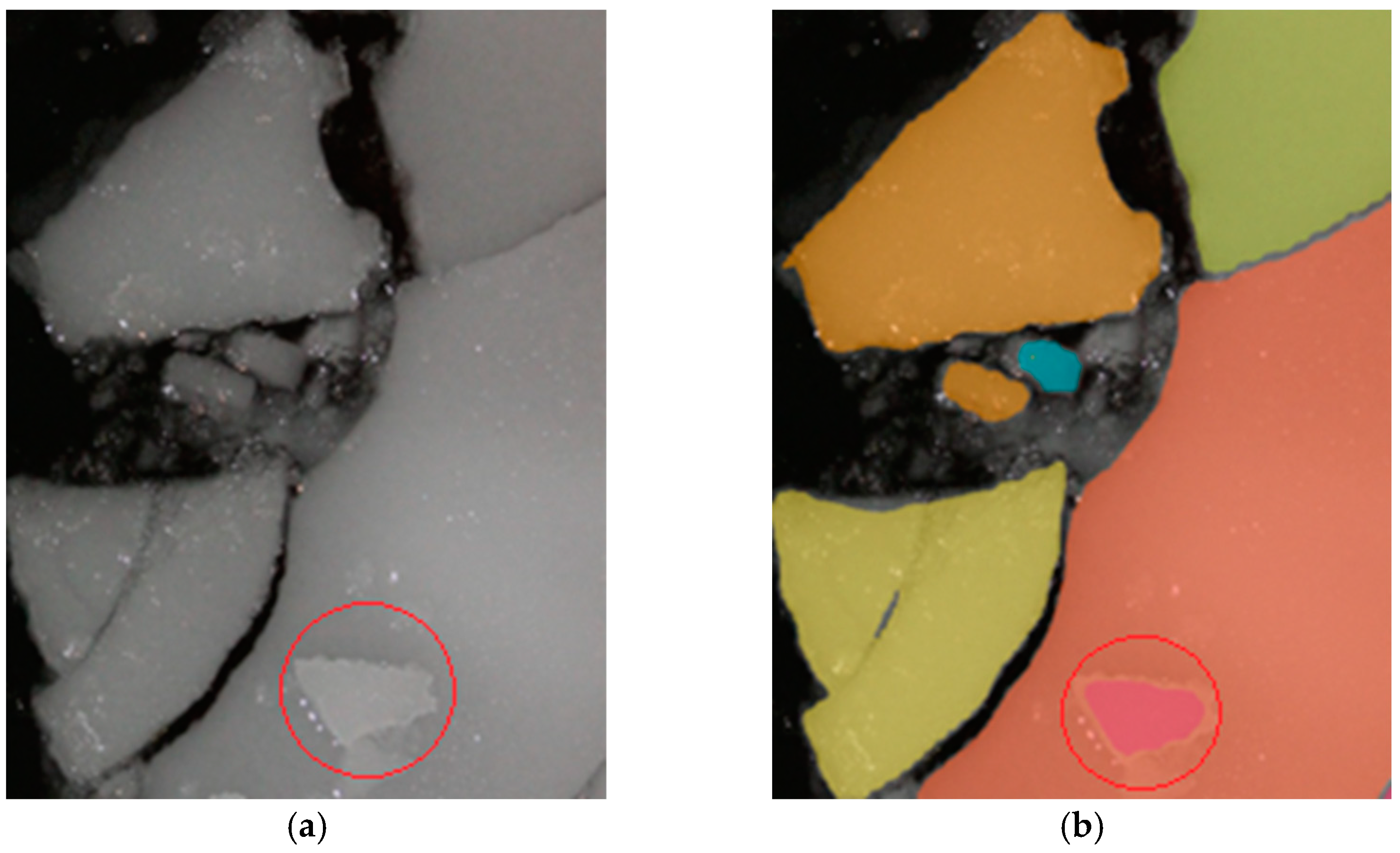
During ice breaking, some crushed ice may overturn and end up on the surface of other floes, as shown in
Figure 4b, which was detected from
Figure 4a. As the model could detect any ice floes in the image, the floes on top of one another would be detected in the results. When calculating the area of all the masks directly, the overlapped area of the ice floes would cause the ice concentration to be overestimated. In practical applications, when icebreakers are breaking the ice, a lot of ice will overturn, and small pieces of ice will often end up on top of larger floes, making it difficult to accurately calculate the ice concentration.
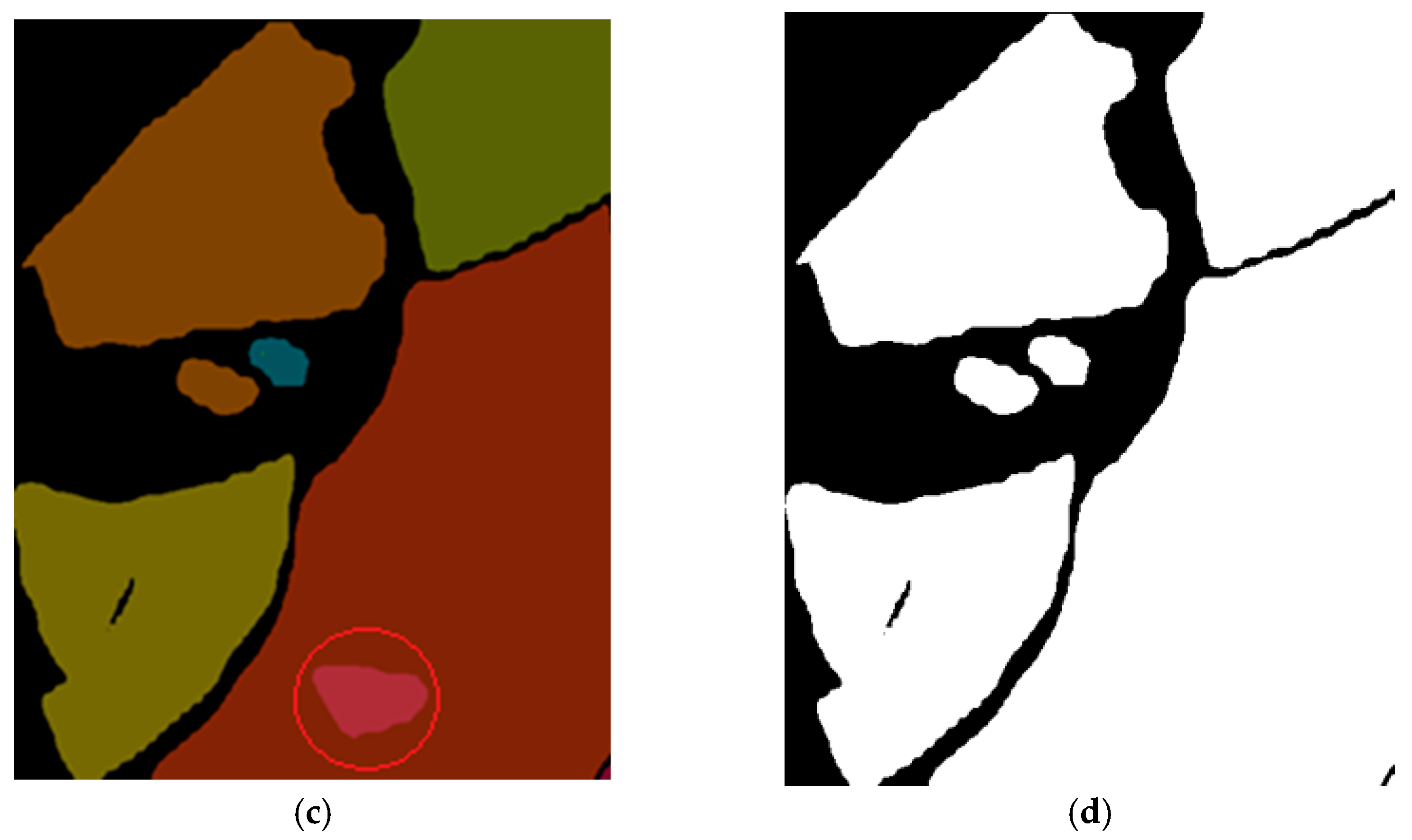
To solve this problem, we used binarization after the ice floe identification. Binarization is an image processing method that classifies all the pixels of an image according to their grayscale values. Pixels with a grayscale value above a certain threshold are displayed as white and those below the threshold are black. However, the output of the detection is a mask overlaid on the original image, which cannot be directly processed through binarization. To address this, we extracted the mask from the detection result of a new image that consisted of all zero tensors, as shown in
Figure 4c. We then converted it into a binarized image, according to the grayscale of each pixel. This allowed us to eliminate the area of an ice floe on top of another, as shown in
Figure 4d, and accurately measure the ice concentration by counting the white pixels in this image.
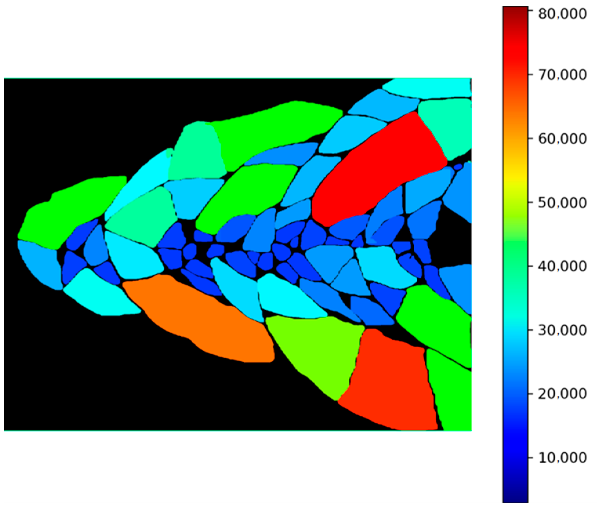
After applying area correction using this method, we calculated the number of pixels belonging to different objects. The number of white pixels represents the area of the ice floes, while the number of black pixels represents the area of the water. Using this information, we collected and labeled all the ice pieces, as shown in
Figure 5. To visualize the sizes more effectively, we defined the size of each ice piece as the number of pixels it occupied. We labeled the ice pieces in different colors, based on the following equation:
where
p is the pixel,
ICE = {
ice(
1),
ice(
2),
ice(
3), …} is a set of detected ice pieces,
Colormap is an RGB color bar from blue to red,
ice(
i)∈
ICE,
size(
i) is the pixel number of
ice(
i), and
size(
ICE) is the pixel number of each ice piece in
ICE. The smaller ice pieces are blue and the larger ice pieces are red. The area of the ice was calculated using Algorithm 2. Additionally, we conducted a test using 100 images to calculate the running time of Algorithms 1 and 2, including a sea ice instance segmentation and calculation of the sea ice concentration. Finally, we found that the speed was 21 FPS, which supports the requirements of real-time detection.
| Algorithm 2. Ice Area Calculation |
| Input: ice segmentation |
| Start algorithm: |
| 1: PIECES←ice segmentation |
| 2: AREA←an empty list to store area of each ice |
| 3: BW ←empty black image |
| 4: for each piece ∈ PIECES do |
| 5: piece←binarization of each mask |
| 6: AREA←area of piece |
| 7: end for |
| 8: INDENX←the number of sorted AREA |
| 9: for i ∈ INDENX do |
| 10: COLOR←get color by Equation (4) |
| 11: pixel of the piece[i]←COLOR |
| 12: BW←BW with colored piece |
| 13: end for |
| 14: IDENTIFICATION←labeled region in BW |
| 15: FLOE←labeled regions in IDENTIFICATION with large sizes |
| 16: BRUSH←labeled regions in IDENTIFICATION with small sizes |
| 17: DISTRIBUTION←floe size distribution |
| 18: return FLOE, BRASH, DISTRIBUTION |
| Output: floe size distribution |
3. Sensitivity Analysis on Annotation and NMS Parameters
When building a dataset and testing the trained model, we found that the sea ice segmentation could be affected by different annotations in the dataset and different settings of the NMS parameter. In this section, we will elaborate on the reasons for this condition and analyze the sensitivity to different annotations and NMS parameters.
3.1. Annotation of Ice Blocks
When collecting ice images, it is necessary to label the ice blocks in these images to inform the computer what constitutes ice, so that it can identify and learn the characteristics of the ice via deep learning. In a previous study [
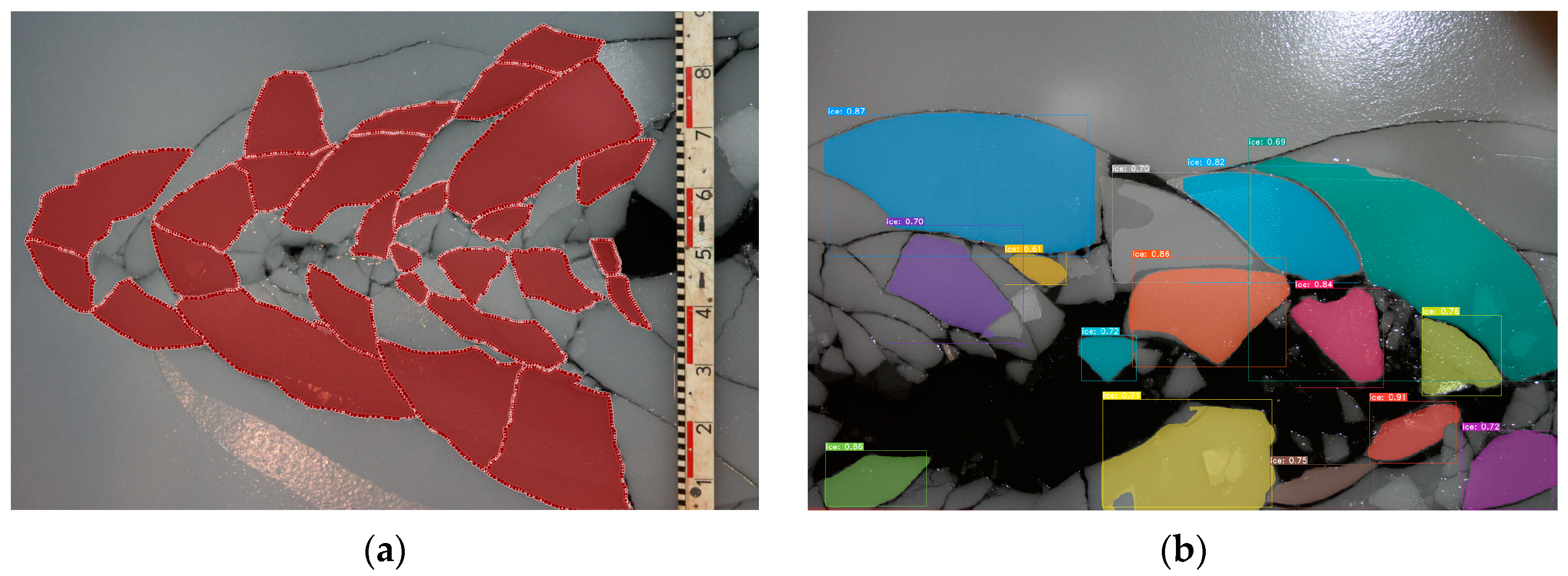
31], YOLACT was used to detect wedge ice and identify circumferential cracks. However, the last dataset used only labeled some wedge-shaped ice, as depicted in
Figure 6a, and did not capture many small ice pieces or the ice around the images. To address this issue, we attempted to use the neural network for identifying the unmarked model ice through a semi-supervised learning approach. Given the large number of ice blocks in each image and the adequate quantity of images, we deemed the dataset to be sufficiently large.
However, when using the model to identify the model ice, a significant amount of model ice could not be segmented due to the network characteristics of YOLACT. The convolution layer outputted a feature vector through the full connection layer, which may have had shape features aligned with the model ice boundaries. The detection result was mostly ice that had a similar shape to the labeled ice in the training set, as shown in
Figure 6b. Ice blocks of other shapes could not be identified and the mask could not cover the ice completely. In the previous task, detecting wedge-shaped ice and extracting circumferential cracks was sufficient to meet the task requirements. However, the task of this study was to calculate the ice concentration and floe size distribution; therefore, all the ice blocks must be detected, regardless of their shape. Hence, the data set was not suitable for this task.
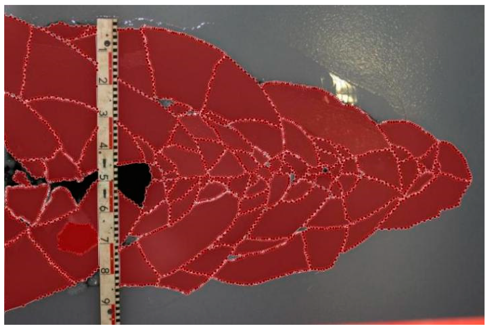
Based on this experience, we relabeled the model ice to eliminate the above-mentioned issues. We mainly relabeled the ice that was not labeled in the previous labeling process, as shown in
Figure 7. In the new data set, we labeled model ice of different shapes to create various training samples. This approach ensured that the model could identify ice of different shapes.
After conducting multiple training tests, we created an instance segmentation dataset specific to sea ice image processing. This dataset could be used to train various models to achieve different functions and the trained model could also be utilized for detecting ice in tanks and open water.
3.2. Recommendation for NMS Parameters
Based on the images captured from the ice tank and open water, ice blocks tend to be in close contact in areas with a high ice concentration. This is in contrast to other object instance segmentation tasks, such as identifying people or cars, where objects generally do not make such close contact. The original YOLACT network can effectively segment the objects in images with generic parameters.
Non-maximum suppression (NMS) acts like a high-pass filter in the YOLACT network, as shown in
Figure 1. It filters out boxes with a lower confidence by first sorting all the prediction boxes
B in the same class, then selecting the prediction box with the highest score
S to calculate the IoU with the other prediction boxes in the same class. It then deletes any boxes larger than the threshold until all the boxes are considered. However, when an object is occluded, as illustrated in
Figure 8, the three dashed boxes represent three objects of the same class, while the solid wireframe is a box that frames all three objects together. Despite having the largest IoU threshold
M, the NMS selects the solid wireframe with an IoU value of 0.9 as the first box to be retained. If the IoU threshold of the other boxes and this box is greater than the selected threshold, the NMS will delete the three dashed boxes with accurate positioning but low classification scores, resulting in an inaccurate box selection.
As the instance segmentation of ice blocks differs from other object detections and instance segmentations, the NMS threshold determines the number of ice blocks that can be identified. In other words, if two ice blocks highly overlap, they can only be detected by setting a large NMS threshold to ensure that the box with a lower confidence score is not suppressed.
YOLACT proposed a new method called Fast-NMS to enhance the speed of detection. The ROI position can be obtained by adding the position offset to the anchor position. As per the above analysis, NMS is a commonly used filtering algorithm if the ROI overlaps. Matrix simplification is used to reduce the time in Fast-NMS; however, some accuracy has to be sacrificed. For example, let us suppose there are five ice ROIs—B1, B2, B3, B4, and B5, respectively. Next, the IoU between them is obtained through a matrix operation. The hypothetical results are shown in
Table 1. In the next step, the lower triangle and diagonal elements of the matrix are deleted to obtain the key parameters presented in
Table 2.
Each of these elements satisfies the condition that the row number is less than the column number. Next, the maximum value for each column is taken and the result is (-, 0.8, 0.6, 0.6, and 0.4). Assuming a threshold of 0.5, any two ROIs with an IoU greater than 0.5 should discard the one with a low confidence. According to the maximum value, the columns corresponding to B2, B3, and B4 exceed the threshold; therefore, these three ROIs will be removed in this step.
This is because, as the row number of each element is less than the column number and the sequence numbers are arranged in descending order from high to low confidence, any element greater than the threshold indicates that the ROI corresponding to this column overlaps with the ROI with a higher confidence; therefore, it needs to be removed.
As stated above, B3 is retained because it overlaps too much with B2 (the IoU is 0.6); however, there is a situation where B3 and B2 are the bounding boxes of ice that are closely contacted. There will be some ice that cannot be detected using this method, as shown in
Figure 9a. To address this issue, we use traditional NMS instead of Fast-NMS to build a more suitable network for the ice instance segmentation. In the traditional NMS algorithm, we set the number of examples to consider for NMS as 200, which means that the bounding boxes of the top 200 IoU will be considered. Because the number of ice blocks in the image is usually large, a threshold of 0.01 is set to remove the bounding box with a confidence less than the threshold. Additionally, we set another NMS threshold of 0.5 to filter out the boxes with an IoU overlap less than this threshold. With these parameters, the algorithm can identify the ice in the ice tank well, as shown in
Figure 9b.
4. Case Study
In this section, we will select an image captured on an icebreaker sailing through a cold region, process this image using the methods introduced in the previous section, and calculate the sea ice concentration and floe distribution.
4.1. Extract the Mask of Ice
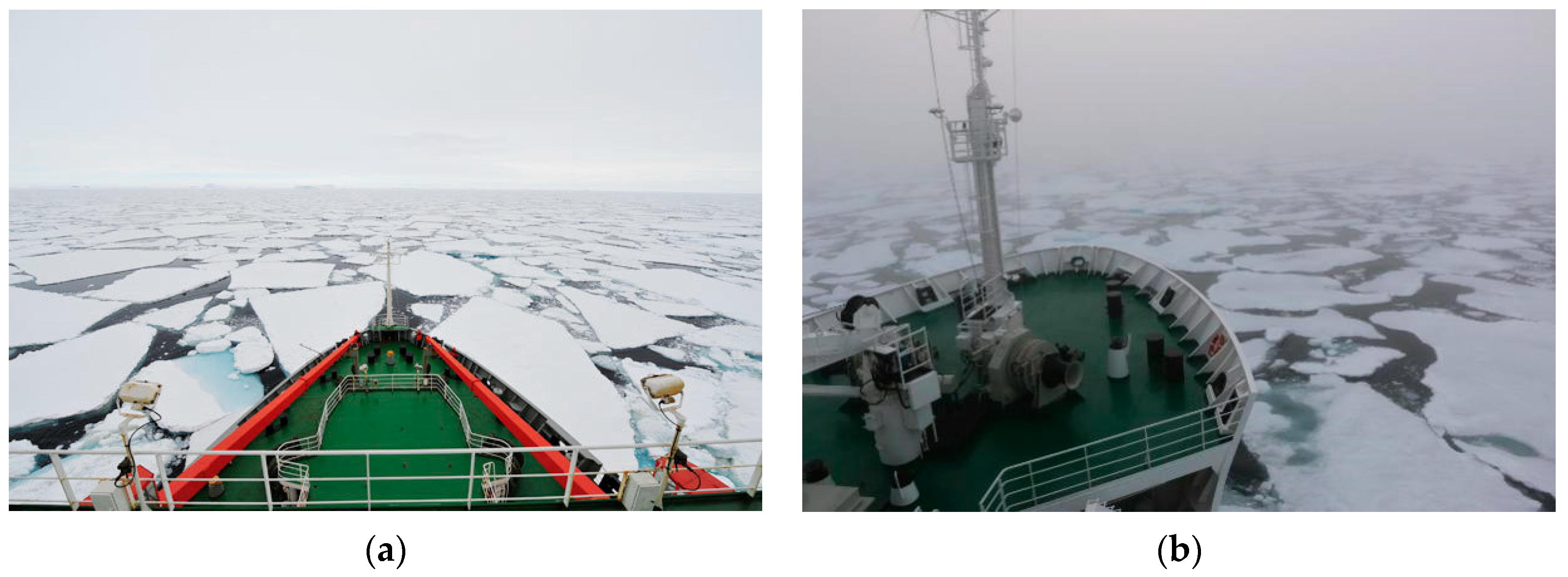
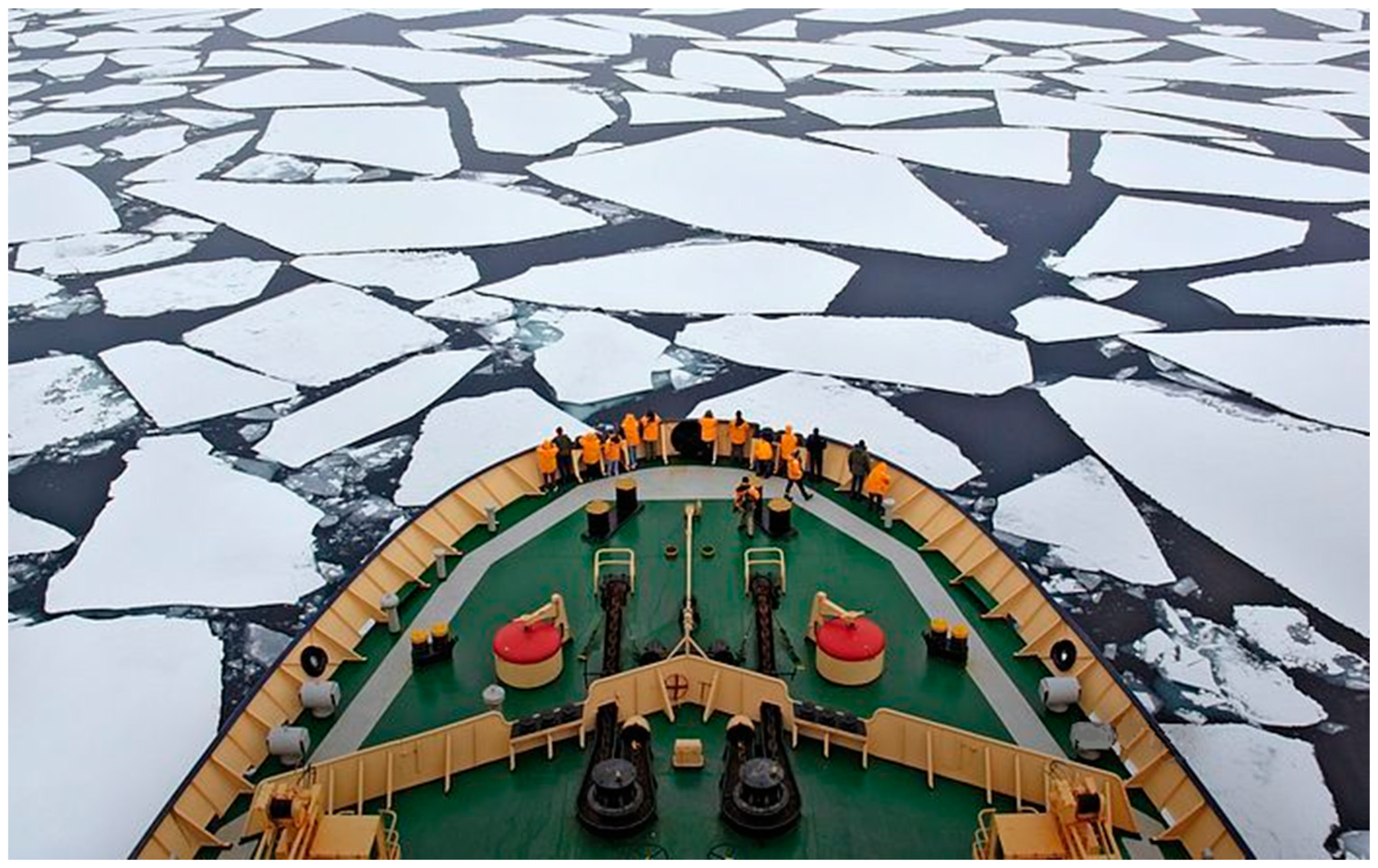
Usually, the camera is placed at the bow of the ship and shoots in the forward direction of the ship at an angle of approximately 45°, as shown in
Figure 10. The sea ice detection algorithm is applied to the image to obtain the mask of the sea ice, which is then converted into a binary format. The number of pixels per mask is calculated to determine the size of the ice floe, and the sum of the pixels for all the masks represents the area of the ice floe in the region that is measured.
When measuring the sea ice concentration in the bow region, the camera must be positioned at a certain angle to capture an image that includes the bow area. To accurately calculate the sea ice concentration, the pixels corresponding to the bow area in the image need to be removed. Additionally, the model must be able to identify different types of ships in the image. To accomplish this, we augment the dataset by adding the training data from ships sailing in cold regions and combine them with the original dataset. The pretraining model we use is based on the model ice. A new model is then trained, which can identify both ships and ice simultaneously.
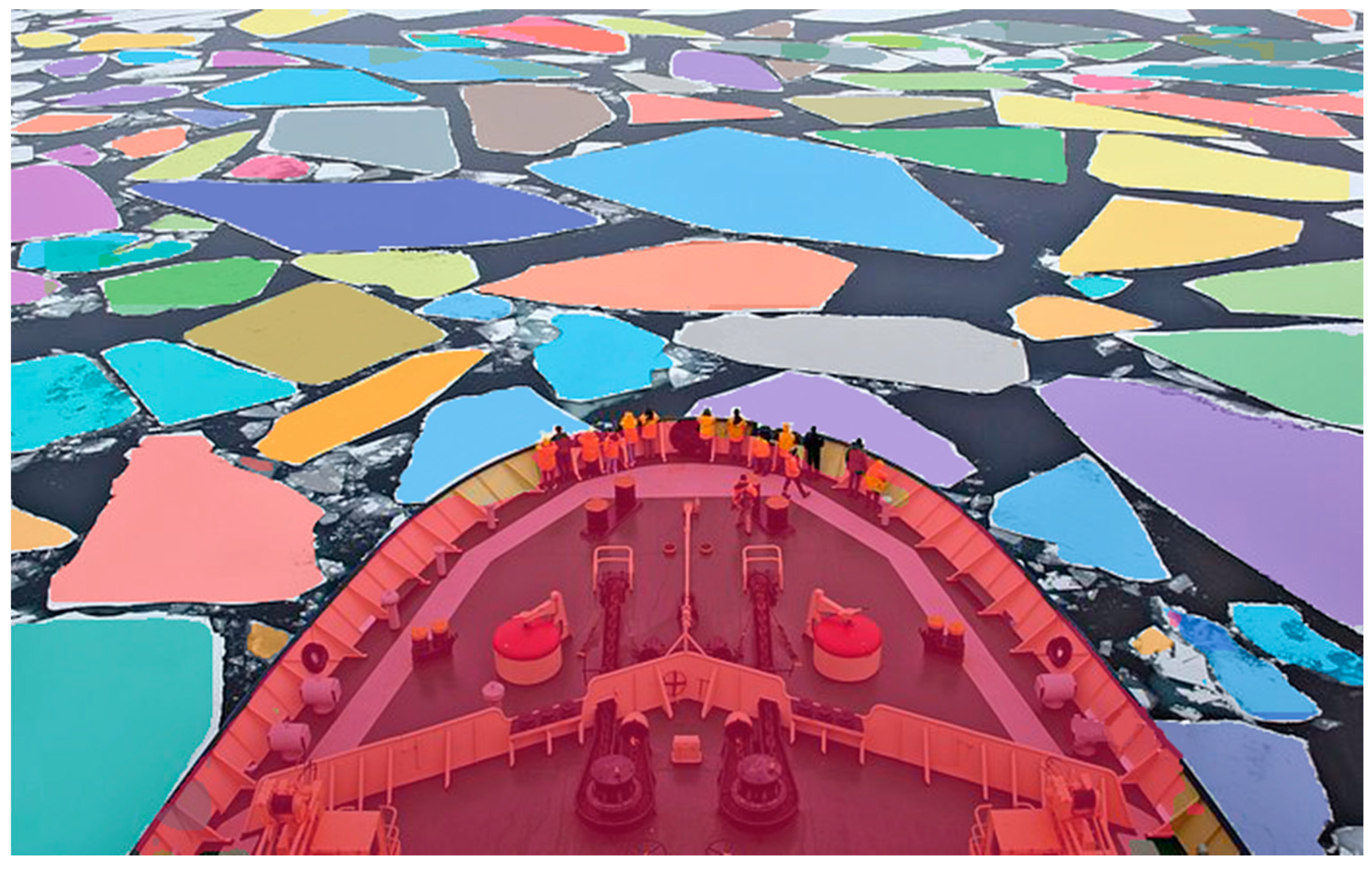
Figure 10 was detected with the new model, as shown in
Figure 11. The sea ice in the bow region is accurately identified. However, due to the shooting angle, the mask of the sea ice detected in the distance is incomplete. The shooting angle not only affects the detection accuracy, but also causes the amount of sea ice detected in the distance to be less than its actual value. In practice, it is difficult to avoid the shooting angle, as this is necessary to ensure that the image contains a large enough area.
4.2. Geometric Calibration
When sailing in polar regions, navigation observations are captured by camera lenses with outward-looking orientations. These cameras take pictures of the bow and shoulder areas; however, to capture a larger area of sea ice around the ship, they are set at a wide angle instead of vertical shooting. However, this can result in inadequate identification results for calculating the size distribution statistics. The calculated area of the ice floes in the far range of the image may be smaller than the actual area, introducing errors into further analyses.
According to [
15,
16], the field of view and shooting angle of the camera can be measured by a sensor and this distortion can be orthorectified. However, in
Figure 10, the actual parameters of the camera are not measured. Therefore, we estimate the shooting angle and field of view based on the statistical similarities between the size distributions of the near and far ranges of the image. In
Figure 10, the shooting angle is approximately 45° and the field of view is 46°. Using this information, we can orthorectify the overall segmentation image and illustrate the algorithm specifically.
As shown in
Figure 11, some ice floes at the far range of the image may not be identified due to distortion. Therefore, a geometric calibration should be performed on the original sea ice image before the ice instance segmentation (Algorithm 1). In this paper, a perspective transformation is used for the geometric calibration, which is a form of projective mapping that projects the picture onto a new viewing plane. Perspective transformation is used to transform objects into straight lines from an original picture, as objects that are straight lines may appear as slashes in the picture. The picture is transformed from the focal plane to the orthorectification plane through a linear transformation and translation, with the transformation equation being as follows:
where (
X, Y, Z) is the coordinate of the focal plane and the transformation matrix is:
.
The transformation matrix can be divided into four parts:
, which denotes the linear transformation, [
a31 a32], which denotes the translation, and [
a13 a23]
T, which leads the perspective. The coordinate of the corresponding point in the transformed picture is (
X′, Y′, Z′). Because we are processing a two-dimensional image, we assume
Z′ = 1 and divide the transformed image coordinates by
Z′, reducing the image from three dimensions to two dimensions. Then, we can obtain the following equation:
Generally, to calculate
X′ and
Y′, we assume
a33 = 1, which yields:
Therefore, given the several points corresponding to the transformation, the transformation equation can be obtained. We choose four points of the original picture, such as (
x0,
y0), (
x1,
y1), (
x2,
y2), and (
x3,
y3). Furthermore, we set four target points as the vertices of the transformed picture: (
X0′,
Y0′), (
X1′,
Y1′), (
X2′,
Y2′), and (
X3′,
Y3′). By substituting these points into Equation (8), we can obtain:
The relationship between (
x,
y) and (
X,
Y) can be found on the basis of [
16]. By substituting the relation equations into (9), the transformed matrix can be obtained.
Once we obtain the transformation matrix, we can perform the perspective transformation on every pixel in the image using Equation (5), as shown in
Figure 12.
If we compare
Figure 10 and
Figure 12, it is clear that the perspective transformation transforms the distorted image into a ”bird’s-eye view” of the ice field, as illustrated in
Figure 13. The view of the ice field has changed from a perspective shot from the ship to a vertical shot over the ice field. The ice in the far range of the picture has been enlarged, while the ice in the close range of the picture has been reduced.
4.3. Sea Ice Concentration and Floe Size Distribution
According to [
16], a brash ice threshold parameter is used to distinguish brash ice from ice floes based on the area of the identified ice. Brash ice is considered to be floating ice fragments no more than 2 m across; thus, ice pieces larger than the threshold are considered to be ice floes, while smaller pieces are considered to be brash ice.
After inputting the picture following the perspective transformation, we obtain the ice floe and brash ice size distributions, as shown in
Figure 14. The color of the ice ranges from blue to red according to the area of the ice blocks, with the brash ice shown in dark blue, smaller floes in light blue, and larger floes in red.
Using the masks of the ice blocks, we can determine the pixel count of the mask and calculate the ice concentration using the equation:
where
MASK = {
m(1),
m(2),
m(3), …} is a set of detected masks and
area(
P) is the pixel number of the whole picture. However, after the perspective transformation is applied to the original picture, the size of the picture changes. Therefore, we calculate the pixel number of
Figure 14 as the new
area(
P). In
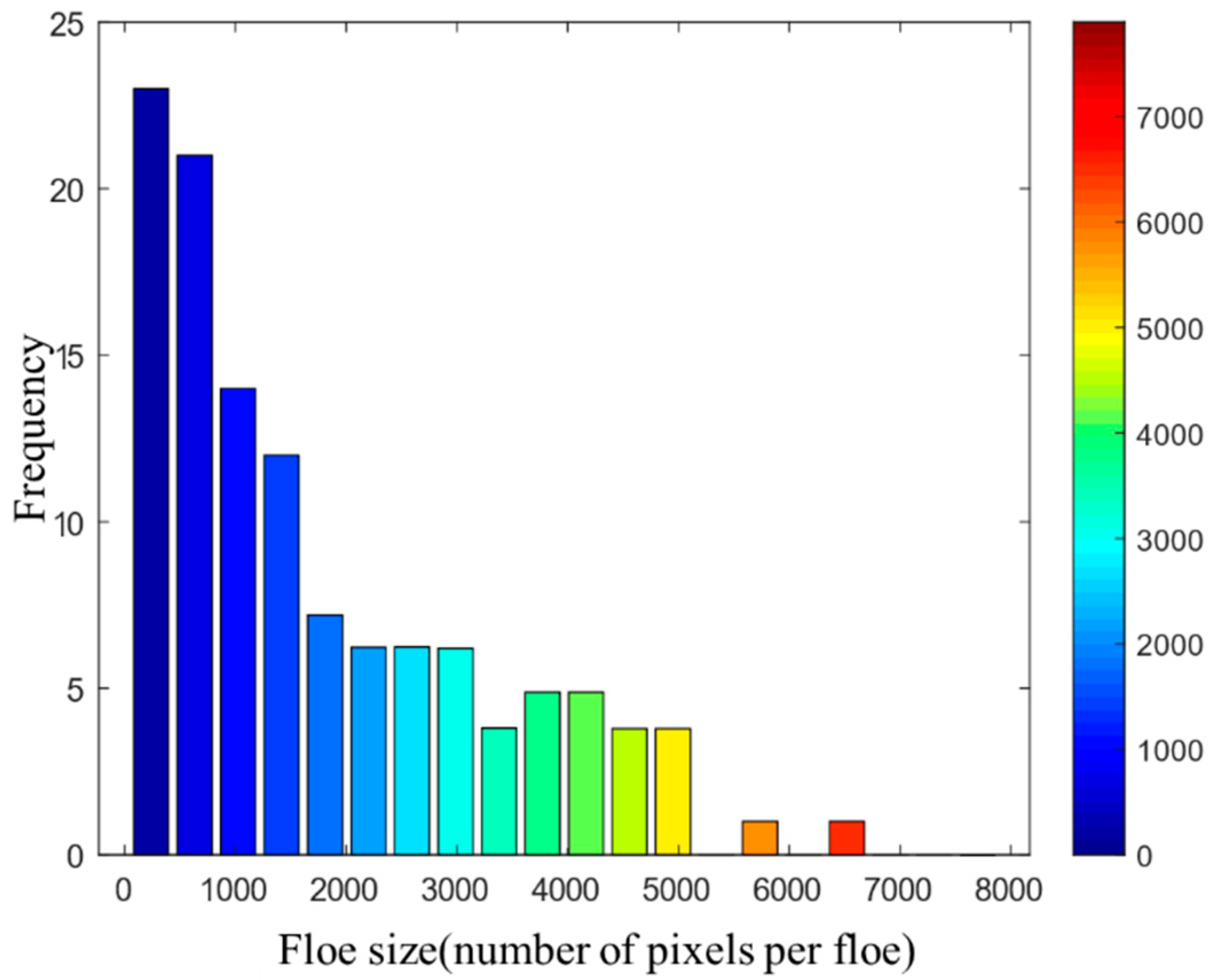
Figure 14, there are 87 ice floes and 1 ship identified. The percentages of coverage are 9.34% of brash ice, 45.12% of ice floes, and 45.53% of water. As the height of shooting the picture is unknown, the actual size of the ice can be calculated based on the number of pixels in the detected sea ice. The ice-floe-distributing histogram is yielded and shown in
Figure 15.
5. Discussion
The method used in this paper took into account the different objects and illuminations in images. Instance segmentation was first used to calculate the ice concentration and size distribution. Shipboard oblique photography is an unavoidable challenge when measuring sea ice. Although possible collisions with ice floes during ice breaking may affect the ice definition, our method is still suitable for regions with low ice concentrations, such as the marginal ice zone. Collisions only occur in regions with heavy ice conditions.
Due to the reflection of light sources on the water and ice, the bright characteristics of light may cause water to be identified as ice floes with threshold segmentation. To train a suitable instance segmentation model to accurately detect sea ice, a dataset of this sea ice was constructed. The dataset contained images of model ice in the ice tank and images of ships sailing through cold regions with varying lighting conditions, allowing the computer to accurately identify the real sea ice. All shapes of the ice and ships in the images were labeled, enabling the model to learn sufficient features. The instance segmentation model trained with this dataset can meet many working conditions in the process of analyzing sea ice images.
6. Conclusions
Compared to remote sensing, images obtained from navigation observations have a higher resolution. Various image processing methods can be applied to these images to obtain important sea ice information, such as sea ice concentration and size distribution in the forward area, which can improve ship handling safety.
To identify the sea ice from images containing both ice and ships and derive the ice concentration, we proposed an algorithm using instance segmentation based on the YOLACT network. In the network, the NMS threshold was adjusted to detect the closely connected ice in high-concentration broken ice fields. The masks outputted from YOLACT were binary, in order to remove the masks of ice blocks that were covered by others, so that the accuracy of the floe size could be calculated. We used perspective transformation in a geometric orthorectification to correct for the situation where ice blocks appeared big when near and small when far and obtained an acceptable sea ice concentration.
The developed methods provided valuable ice information that can be used to improve our understanding of the sea ice in polar regions and navigation safety. However, it is necessary to collect more image data to extend the dataset and quantitatively validate the present method of calculating ice concentration. Images from different working conditions are also needed to provide a basis for comparison with this study and this will be addressed in future research.


