Article

On the Retrieval of Surface-Layer Parameters from Lidar Wind-Profile Measurements

by
Marcos Paulo Araújo da Silva
1,
Andreu Salcedo-Bosch
1,
Francesc Rocadenbosch
1,2,* and
Alfredo Peña
3
1
CommSensLab-UPC, Department of Signal Theory and Communications, Universitat Politècnica de Catalunya (UPC), C/ Jordi Girona, 1-3, 08034 Barcelona, Spain
2
Institut d’Estudis Espacials de Catalunya (Institute of Space Studies of Catalonia, IEEC), 08034 Barcelona, Spain
3
DTU Wind and Energy Systems, Technical University of Denmark, Frederiksborgvej 399, 4000 Roskilde, Denmark
*
Author to whom correspondence should be addressed.
Remote Sens. 2023, 15(10), 2660; https://doi.org/10.3390/rs15102660
Submission received: 4 April 2023 / Revised: 12 May 2023 / Accepted: 16 May 2023 / Published: 19 May 2023
(This article belongs to the Section Atmospheric Remote Sensing)

Abstract

:
We revisit two recent methodologies based on Monin–Obukhov Similarity Theory (MOST), the 2D method and Hybrid-Wind (HW), which are aimed at estimation of the Obukhov length, friction velocity and kinematic heat flux within the surface layer. Both methods use wind-speed profile measurements only and their comparative performance requires assessment. Synthetic and observational data are used for their quantitative assessment. We also present a procedure to generate synthetic noise-corrupted wind profiles based on estimation of the probability density functions for MOST-related variables (e.g., friction velocity) and the statistics of the noise-corrupting perturbational amplitude found during an 82-day IJmuiden observational campaign. In the observational part of the study, 2D and HW parameter retrievals from floating Doppler wind lidar measurements are compared against those from a reference mast. Overall, the 2D algorithm outperformed the HW in the estimation of all the three parameters above. For instance, when assessing the friction-velocity retrieval performance with reference to sonic anemometers, determination coefficients of ρ 2 D 2 = 0.77 and ρ H W 2 = 0.33 were found under unstable atmospheric stability conditions, and ρ 2 D 2 = 0.81 and ρ H W 2 = 0.07 under stable conditions, which suggests the 2D algorithm as a prominent method for estimating the above-mentioned surface-layer parameters.

Graphical Abstract

1. Introduction

Wind energy is one of the most cost-efficient renewable power-generation technologies nowadays. Accordingly, the amount of onshore and offshore wind farm being installed worldwide has greatly increased over the last years [1]. Nevertheless, the onshore sector has become comparatively less attractive in terms of wind conditions and capacity factor as well as it has faced resistance by populations from potential deployment areas that may be affected by the farm installation and operation. Hence, the industry development has been moving towards offshore [2,3]. However, despite the abundant wind resource that can be found over the seas, offshore wind farm harvesting remains more expensive than its onshore counterpart. Additionally, the site’s feasibility still relies on offshore meteorological masts (metmasts), which are very expensive to install and maintain [4].
During the last decade, floating Doppler wind lidars (FDWLs) have emerged as the wind-energy-industry preferred solution to replace the metmast because of their accuracy and attractive cost-benefit of installation and maintenance. Many studies have shown that 10 min averaged wind-speed measurements from FDWLs are numerically equivalent to reference observations from anemometers or fixed Doppler wind lidar (DWL) [4,5,6]. However, FDWLs cannot measure a number of the atmospheric parameters that instruments mounted on meteorological masts can, which restrains commercial acceptance of FDWLs as stand-alone sensing instrument.
The surface layer is the lowest part of the atmospheric boundary layer (ABL) where turbulent fluxes vary by less than 10% of their magnitude [7]. A measure of atmospheric stability is the Obukhov length, which has been used to extend the logarithmic wind profile to account for atmospheric stability conditions [8]. The Obukhov length is directly related and very sensitive to the friction velocity. The latter is a fundamental velocity scale of atmospheric flow and can also be used to estimate the wind-speed standard deviation, which determines, together with the mean wind speed, turbulence intensity [9]. The role of the Obukhov length and friction velocity has been investigated in different wind-energy studies related to wind-turbine wake modelling [10], power production [11], and structural loading (e.g., wind-turbine aeroelastic design) [12]. It is worth noting that the eddy-covariance method, from which one can derive the friction velocity and heat flux is currently the most accurate way to derive the Obukhov length [7,13]. Estimations, however, can be alternatively performed using, e.g., the Richardson number [14].
Multiple sensors, such as sonic anemometers installed on metmasts, provide high-frequency measurements, which can be used to derive turbulent fluxes. Other sensors can provide air-pressure and air-humidity observations. However, alternative methods are needed in scenarios with limited instrumentation [5,15,16,17,18,19,20]. A good number of these methods use Monin–Obukhov similarity theory (MOST).
The MOST wind-profile model can be understood as a generalisation of the log-law model, and accordingly, it also implies a wind-speed profile that monotonically increases with height [13,15]. However, differently from the log-law model, which is only valid under neutral conditions, the MOST model takes into account the atmospheric stability influence over the profile [13]. However, MOST is not exempt from limitations. Thus, the MOST wind-profile model is valid within the surface layer only. Therefore, it can normally be used to predict wind speeds up to approximately 100 m [8,21]. Moreover, different authors [22,23] have shown that the traditional MOST is not applicable to swell-dominated seas. Swell waves (often referred to as surface gravity waves) consist of wind-generated waves over a fetch of water that are not greatly affected by the local wind at that time and that are usually characterised by a relatively long wavelength. Jiang [24] also showed that the swell impact on wind profiles is more pronounced under neutral or stable boundary-layer conditions and low winds, and less so under unstable (convective) conditions.
The methods for estimation of surface fluxes of momentum and heat (i.e., surface-layer parameters) by [16,20] require both temperature and wind-speed measurements, and that by Klug [17] the aerodynamic roughness length in addition. When looking for studies utilising only wind-speed measurements as a feasible alternative to be applied using FDWL observations, the number of surface-layer-retrieval methods are limited to four [5,15,18,19]. Nevertheless, the reliability of the optimisation method proposed by Lo [19] can be considered questionable because of different mathematical issues reported by Zhang [25]. Of the remaining three methods, the recent one by Basu [15] (2019)–the so-called Hybrid-Wind (HW) method–is an enhanced version of the Swinbank [18] (1964), in which the surface-layer wind profile follows an exponential profile instead of MOST [5,8,26,27,28]. HW estimates the Obukhov length from three levels of wind speed measurements. Once the Obukhov length is obtained, the friction velocity and surface heat flux can be derived. In contrast to HW, the 2D method by Araújo da Silva et al. [5] (2022) enables a simultaneously retrieval of the Obukhov length and friction velocity by using a two-dimensional (2D) parametric-solver algorithm. Moreover, the 2D algorithm can be extended to any number of measurement heights describing the wind profile.
In the present work, we aim at assessing the performance for retrieval of surface-layer parameters of both the 2D and HW methods. Aligned with this aim is to identify the most reliable method relying on FDWL observations only, which is to foster commercial acceptance of the FDWL as the wind-energy-industry preferred solution to replace the offshore metmast. Performance evaluation is twofold: First, we use reference synthetic noise-corrupted wind-profile realizations with characteristic parameters inherited from FDWL observational datasets. Second, we use sonic-anemometer estimates from the IJmuiden metmast. Focus is also given to the stand-alone capability of these methods for atmospheric stability estimates.
This paper is structured as follows. Section 2 presents the observational campaign at the IJmuiden site. Section 3 reviews MOST and revisits the 2D and HW retrieval algorithms. Section 4 studies the comparative performance of both the 2D and HW methods as a function of the noise-corrupting intensity and stability condition with reference to synthetic and observational data. Section 5 provides concluding remarks.

2. Materials

The IJmuiden observational campaign was carried out in the Dutch North Sea (52.848°N, 3.436°E) over 82 days from April to June 2015, aimed at validating the EOLOSTM FDWL against the IJmuiden metmast [5]. Figure 1 shows the IJmuiden’s mast and FDWL geographical positions in the North Sea. The FDWL was collocated 200 m next to the mast and 85 km from the Netherlands coast. A ZephIRTM 300 focusable continuous-wave Doppler lidar installed at the FDWL buoy measured wind speed profiles at four levels, 25, 38, 56, and 83 m above the Lowest Astronomical Tide (LAT). Hereafter, all height values will be assumed as height above LAT. Reference wind profiles were provided by the sonic and cup anemometers installed at 27, 58.5, and 85 m in the IJmuiden mast.

3. Methods

3.1. MOST Wind Profile

According to MOST, the diabatic wind profile (i.e., under non-neutral conditions) within the surface layer is expressed as
U M O S T ( z ) = u * κ ln z z 0 Ψ m z L ,
where z is the height [m], u * is the friction velocity [m/s], κ 0.4 is the Von Kármán constant, z 0 is the roughness length, L is the Obukhov length, and Ψ m z L is a stability-correction function [13,29]:
Ψ m z L = β z L z L > 0 ( stable ) 0 z L = 0 ( neutral ) 2 ln ( 1 + x 2 ) + ln ( 1 + x 2 2 ) 2 arctan ( x ) + π 2 z L < 0 ( unstable ) ,
where x = 1 γ z L 1 / 4 , and β = 6.0 and γ = 19.3 are empirical constants suggested by Högström [30], which where already validated by [5,8] for the IJmuiden site.
The Obukhov length is a scaling parameter that is proportional to the height above the surface layer at which buoyant factors first dominate over mechanical production of turbulence [13]. The Obukhov length can be computed from:
L = θ ¯ v u * 3 κ g ( w θ v ¯ ) s ,
where θ ¯ v is the virtual potential temperature, w is the vertical wind component, ( w θ v ¯ ) s is the surface-layer virtual kinematic heat flux, and g = 9.8 m/s 2 is the gravitational acceleration. The overbar indicates average over time (normally 10 min). The “prime” in w and θ v denotes the fluctuating part of these components, i.e., the deviations from their respective mean values.
Offshore, the roughness length can be modelled through the Charnock’s relationship as [31]
z 0 = α c u * 2 g ,
where α = 0.012 is the Charnock’s constant and g = 9.81 [m/s 2 ] is the gravitational acceleration [8,32]. By inserting Equation (4) into Equation (1), the latter equation can be written as a function of only the variables Obukhov length and friction velocity as
U ( z , L , u * ) = u * κ ln z α c u * 2 g Ψ m z L .
Despite the simplicity of Charnock’s model (Equation (4)), this model has the advantage of only depending on one of the variables that are being searched for ( u * ). Physically, because of the overall low roughness over water, the sensitivity of any retrieval method to the roughness length per se is very small (and hence to the Charnock’s constant).
Figure 2 revisits MOST, i.e., Equation (1), for different stability conditions and sensitivity analysis in these two variables. Figure 2a shows that the wind profile in neutral stability conditions appears as a straight line with logarithmic height. In stable conditions the wind profile is concave downwards, while in unstable conditions is concave upwards. Note that MOST models wind profiles in which the wind speed monotonically increases with height, i.e., the wind profile has positive gradients at all heights [15,33]. Figure 2b,c show that the wind profile is much more sensitive to friction velocity u * than to the Obukhov length L. The wind profile is virtually insensitive to perturbations in the sea roughness length.

3.2. Surface-Layer Parameter Retrieval Methods Based Solely on Wind Speed Profiles

3.2.1. The 2D Method

The 2D parametric solver algorithm simultaneously estimates the friction velocity, u * , and Obukhov length, L, relying on MOST and wind-profile measurements only [5]. The algorithm estimates model parameters (L, u * ) by minimising the norm of residuals between the model vector U M O S T ( L , u * ) , Equation (5), and the observed wind-profile vector U o b s , via constrained least-squares optimisation. Thereby, the optimisation problem is formulated as
( L ^ , u ^ * ) = arg min L , u * | | U o b s U M O S T ( L , u * ) | | 2 .
Two optimisation branches, one for Ψ m z L > 0 and another for Ψ m z L < 0 , are considered for enhancing the sensitivity of the algorithm and avoiding the asymptotic discontinuity, | Ψ m z L | 0 . The branch that yields the smallest residual norm is chosen as the solution. Once L and u * are obtained, the heat flux is estimated from the definition of L (Equation (3)) as
w θ ¯ = θ 0 u * 3 κ g L ,
where θ 0 = 300 K is assumed as the reference potential temperature. Following [33], Equation (7) is just a plausible approximation of the surface-layer heat flux ( w θ v ¯ ) s in Equation (3) when temperature measurements are not available as is the case of relying solely on wind-speed (e.g., FDWL) measurements.

3.2.2. The Hybrid-Wind Method

The HW method is a MOST-based algorithm that primarily retrieves the Obukhov length from three height levels of a horizontal wind speed (HWS) profile [33]. Given the Obukhov length and MOST profile Equation (1), the friction velocity and heat flux are also obtained. Because the HW method is also reliant on MOST, the assumption of monotonic wind behaviour is inherent to the method (Section 3.1).
The HW reduces the number of MOST wind-profile parameters from three, namely, Obukhov length (L), friction velocity ( u * ) and roughness length ( z 0 ), to one primary parameter, the Obukhov length (L), by resorting to the ratio of the vertical wind-speed differences, which are formulated as [33]
Δ U 21 = U ( z 2 ) U ( z 1 ) = u * κ ln z 2 z 1 Ψ m z 2 L + Ψ m z 1 L ,
Δ U 31 = U ( z 3 ) U ( z 1 ) = u * κ ln z 3 z 1 Ψ m z 3 L + Ψ m z 1 L ,
where U ( z i ) is the HWS at the height z i . Then, the ratio of wind speed differences is defined as
R ( L ) = Δ U 31 Δ U 21 = ln z 3 z 1 Ψ m z 3 L + Ψ m z 1 L ln z 2 z 1 Ψ m z 2 L + Ψ m z 1 L .
The ratio R ( L ) is only function of Obukhov length L, which is retrieved via a non-linear least squares that fits the observed to the modelled vertical wind-speed ratio. Thus, the optimisation problem for the HW method is formulated as
( L ^ ) = arg min L | | R o b s R ( L ) | | 2 ,
where R o b s is the observed vertical wind-speed ratio and R ( L ) is the modelled one given by Equation (10).
Eventually, this retrieved Obukhov length L ^ is used to solve friction velocity u ^ * from the formulation of HWS differences Δ U 31 ( u * , L ) and Δ U 21 ( u * , L ) expressed in Equation (8) above via ordinary linear least squares. After estimating L and u * the heat flux can also be estimated via Equation (7). This procedure is identical for the 2D method once L and u * are known.

3.3. Observational Reference Retrievals

Ten-minute averages of the observations from the IJmuiden metmast are used to determine the reference data as:
(i)
Reference Richardson-number-estimated Obukhov length, L R i .—Because high-frequency temperature data from the sonic anemometers were not stored, the Obukhov length was estimated via bulk Richardson number using the methodology proposed by [14]. L R i was computed as described in [5] (Section 3.4, pp. 7–9) and summarised here in Appendix A.
(ii)
Reference friction velocity.—The sonic anemometers were installed at 85 m in height, which may well lie above the surface layer. Therefore, two approximate reference friction-velocity values were computed:
(a)
The local friction velocity at 85 m via the sonic-anemometer measurements as [7]:
u * s o n i c = u w ¯ 2 + v w ¯ 2 1 / 4 ,
where u, v and w denote the longitudinal, lateral and vertical wind components, respectively.
(b)
The so-called 1D friction velocity, denoted u * 1 D . The 1D friction velocity was numerically derived by solving Equation (5) for u * given the Richardson-number-estimated Obukhov length ( L R i , refer to Appendix A) and the measured wind-speed at 27 m, which is the lowest height available from the metmast. Accordingly, u * becomes the only unknown in Equation (5) (hence the one-dimensional (1D) suffix used), which is solved via least-squares optimisation.

3.4. Synthetic Data Generation

As mentioned in Section 3.3 our observational references are not exempt from limitations. Thus, in spite of the large number of measurement records available in IJmuiden, the campaign was limited to estimates of the Obukhov length computed using the Richardson-number approximation as a proxy, and subject to MOST-perturbational noise levels within a given amplitude span (to be computed) specific of this campaign. Therefore, the motivation to employ synthetic data is double: (i) to have “truth” wind profiles by which to numerically assess the performance of the 2D and HW methods under the MOST assumption, and (ii) to benefit from a much wider perturbational noise-level span (from virtually 0 to 100%, to be formulated next) than the specific one of IJmuiden.
The numerical simulations were performed using the High Performance Computing environment CALCULA. CALCULA uses as a basis the resource management system Slurm Workload Manager, a scheduler of open source tasks widely used in supercomputing environments, and the system of GlusterFS distributed files for data management. Furthermore, 2D and HW retrieval accuracies were examined by using random sets of synthetic wind profiles, U s y n ( z ) , generated for different atmospheric conditions. Monte-Carlo simulation was used to generate synthetic pairs ( u * s y n , L s y n ) compliant with MOST (Equation (1)). This is explained next:

3.4.1. Generation of Obukhov Length and Friction Velocity Random Pairs

The variables Obukhov length and friction velocity are physically related via Equation (3). Consequently, random sets for these variables cannot be created using the customary assumption of independent Gaussian random variables. To circumvent this problem, in Equation (3) we recognise that L is proportional to the cube of the friction velocity and the ratio θ ¯ v / ( w θ v ¯ ) s , which is denoted factor c in what follows. Hence, Equation (3) can be rewritten as
L = c k g u * 3 .
From Equation (12) above, it follows that Obukhov length L is unambiguously defined by friction velocity u * and factor c or, equivalently, that random values for u * and c must be generated from the Probability Density Functions (PDFs) of independent random variables U * and C, respectively. Here upper-case letters denote random variables and lower-case letters denote the values for these variables. Because the PDFs for random variable friction velocity U * and random variable C-factor are a priori unknown, they have to be estimated. This was done from the whole set of IJmuiden metmast measurements recorded during the campaign (8263 records, hereafter “the statistical sample”) as follows: the PDF for U * was approximated by that of local friction velocity U * s o n i c computed via Equation (11) over the statistical sample. The PDF for C was derived from the estimates of this variable computed as C k g L R i U * s o n i c 3 over the statistical sample, where L R i is the Richardson-number-estimated Obukhov length (Appendix A).
Different PDFs models were experimentally fitted to the estimated friction velocity U * and factor-C distributions in order to obtain the PDFs that best described the observations. As a result, it could be observed that both U * and C followed a log-normal distribution or the combination of a log-normal with a folded version of it. The log-normal PDF for a random variable X is formulated as
f X ( x ) = 1 σ X 2 π e [ ln ( x ) μ X ] 2 2 σ X 2 , x > 0 ,
where μ X and σ X are the PDF constitutive parameters.
Because the log-normal PDF is positive defined, it becomes an appropriate distribution to describe the friction velocity PDF, denoted f U * ( u * ) . In contrast, because variable C can have positive and negative values, its PDF is defined log-normal piecewise as
f C ( c ) = f C p ( c p ) , c p = c , i f c > 0 , f C n ( c n ) , c n = c , i f c < 0 ,
where f C p ( c p ) and f C n ( c n ) are the log-normal ( X = C p , Equation (13)) and folded log-normal ( X = C n ) PDFs associated to positive and negative values of C, denoted c p and c n , respectively. As mentioned, upper-case letters denote random variables and lower-case letters denote values for these variables. In what follows, this notation formality is skipped unless otherwise necessary for understanding.
By fitting: (i) Equation (13) PDF with X = U * to the statistical sample of local friction-velocity values measured at 85 m ( U * s o n i c , Section 3.3), and (ii) Equation (14) PDF to the C-factor sample computed as C k g L R i U * s o n i c 3 , then PDF characteristic parameters, μ X = μ u * and σ X = σ u * for f U * ( u * ) , and μ X = μ C , p , μ C , n and σ X = σ C , p , σ C , n for f C ( c ) can be estimated. Once PDFs f U * ( u * ) and f C ( c ) are characterised, random values u * s y n and c s y n can be generated computationally. Most data-processing software packages provide built-in algorithms able to generate log-normal-distributed random values. Alternatively, log-normal distributions can be obtained by transforming uniformly distributed random values through the inverse log-normal cumulative distribution function. Thus, log-normal distributed values y can be obtained using the transformation [34]
y = e μ + 2 σ 2 e r f 1 ( 2 x 1 ) ,
where x are random values from a uniformly distributed random variable, and e r f 1 is the inverse Gauss error function. Once random values u * s y n and c s y n have been generated, L s y n values can readily be computed from Equation (12).

3.4.2. Generation of Synthetic Wind Profiles

Model wind profiles, U M O S T ( z ) , can be generated from the pairs ( u * s y n , L s y n ) via MOST (Equation (1)). However, model profiles are noiseless and, in practice, there are always deviations from the MOST profile. In order to emulate these deviations, height-independent zero-mean Gaussian-noise realizations are added to the noiseless model profiles. This can be expressed as
U s y n ( z i ) = U M O S T ( z i ) + σ n ν ( z i ) , i = 1 N ,
where U s y n is the noise-corrupted wind profile (hereafter, the synthetic wind profile), U M O S T is the MOST profile (Equation (1)), ν is zero-mean, unit-standard-deviation Gaussian noise, z i is the i-th metmast anemometer-measurement height ( z i = 27 , 58.5 , 85 m, Section 2), and N is the number of measurements heights.
We quantify the intensity of these perturbations by means of the normalised root-mean-squared error ( N R M S E , hereafter, the normalised noise level), which is defined in percentage units as
N R M S E = 100 × 1 U m a s t ¯ 1 N i = 1 N [ U M O S T ( z i ) U m a s t ( z i ) ] 2 ,
where U m a s t is the measured wind profile from the metmast anemometers at height z i .
The noise-corrupting amplitude is defined as the standard deviation,
σ n = N R M S E U m a s t ¯ 100 ,
where the overbar indicates average over the measurement heights 27, 58.5 and 85 m. From Equation (18), it follows that the normalised noise level (Equation (17)) quantifying the noise-corrupting perturbational amplitude in synthetic wind profiles can also be rewritten as N R M S E = σ n U m a s t ¯ 100 [ % ] .
The block diagram in Figure 3 summarizes the procedure for synthetic wind-profile generation. First, random pairs ( u * s y n , c s y n ) are generated from PDFs f U * ( u * ) and f C ( c ) as described in Section 3.4.1. Then, L s y n values are computed from u * s y n and c s y n values via Equation (12). Next, each “seed” pair ( u * s y n , L s y n ) is used to produce a noiseless MOST profile, U M O S T ( z ) , via Equation (1). Finally, zero-mean, σ n -standard-deviation Gaussian noise ν ( z ) (Equation (18)) is added to the model wind profile U M O S T ( z ) in order to yield noise-corrupted wind profile U s y n ( z ) .
The absolute relative error between the estimated and the synthetic friction velocity, the latter taken as reference, is computed as:
ϵ u * = | u ^ * u * s y n | u * s y n
where u ^ * is the estimated friction velocity and u * s y n is the synthetic one.

4. Results and Discussion

We study the comparative performance of 2D and HW methods as a function of the noise level and atmospheric stability conditions. First, Section 4.1 shows the synthetic generation of the friction-velocity-to-Obukhov-length distribution proxy for the IJmuiden dataset, which becomes our synthetic “truth” reference for comparison. Section 4.2 and Section 4.3 evaluate the performance of the 2D and HW methods with reference to synthetic and observational data, respectively.

4.1. On the Generation of Synthetic Wind Profiles

In order to assure realistic synthetic data generation, we considered the measurements from IJmuiden campaign. The IJmuiden campaign consisted of 8263 measurement records after outlier rejection (refer to [5], pp. 10–11 for details; in short, rejected measurements were: (i) FDWL-measured HWS values lower than 2 m/s and higher than 80 m/s, and (ii) FDWL-measured spatial variation values higher than 0.055).
Retrieval of PDF characteristic parameters.—First, the PDFs for the friction velocity, f U * ( u * ) , and C-factor, f C ( c ) , were inferred from the measured distributions of the sonics-derived friction velocity ( U * s o n i c ) and Richardson-number-estimated Obukhov length ( L R i ) as described in Section 3.4. When fitting model PDF Equations (13) and (14) to the measured friction-velocity and C factor, characteristic parameters of U * and C-factor distributions were obtained. Once f U * ( u * ) and f C ( c ) were found, random pairs ( u * s y n , L s y n ) could be generated. Please refer to Appendix B for further details and quality assurance of the retrieved characteristic parameters.
Estimation of the noise level distribution.—In Section 3.4.2 we found that the normalised noise level ( N R M S E , Equation (17)) could be understood as an indicator of the average noise level in the wind profile. In order to estimate typical values for this normalised wind-perturbance intensity indicator, we computed the normalised RMSE between the MOST-predicted and metmast-measured wind profiles.
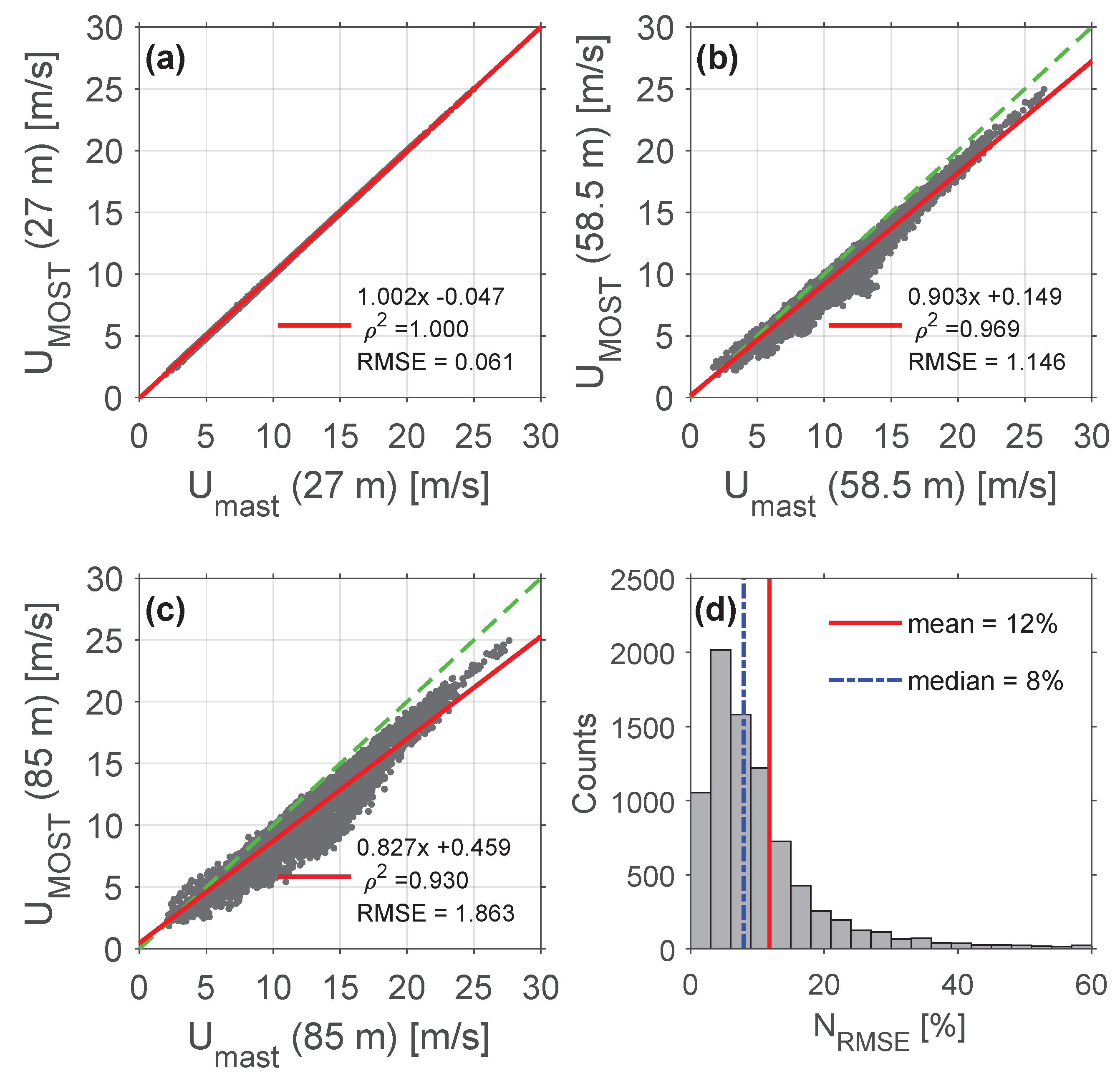
The MOST-predicted wind profile was computed through the 1D friction velocity, u * 1 D , and Richardson-number-derived Obukhov length, L R i , in Equation (1) (refer to Section 3.3 and Appendix A). Figure 4 compares the MOST-predicted to the metmast-measured wind speed at the three measurement heights (Figure 4a–c) and derives the resulting normalised RMSE distribution (Figure 4d). The virtually ideal 1:1 regression line obtained at 27-m height (Figure 4a) is because u * 1 D was numerically retrieved using the metmast-measured wind-speed at this same height. It could be observed experimentally that the MOST model uncertainty increases with height demonstrating MOST limitations above the surface layer, which is evidenced by decreasing linear regression indicators. By merging all the measurement samples from Figure 4a–c into Equation (17), the histogram bar chart for the normalised RMSE could be derived (Figure 4d). The normalised RMSE observed spanned from 0 to 60% and its mean and median values were, N R M S E = 12 % and 8 % , respectively, which is descriptive of the statistical noise levels found in real practice in IJmuiden.

4.1.1. Generated Synthetic Data Outlook

To begin with, a dataset consisted of 5000 randomly-generated samples, where each sample stands for one pair friction velocity and Obukhov length, ( u * s y n , L s y n ) , and its respective noisy wind profile. MOST profiles were generated using the same measurement heights as for the FDWL (i.e., 25, 38, 56, and 85 m, see Section 2). To obtain a sample noisy wind profile, a noise realization with noise level N R M S E was added to the MOST profile (Equation (16)). Based on the measured distribution of the normalised noise level ( N R M S E ) shown in Figure 4d, in our simulations, we considered 20 noise levels (Equations (17) and (18)) spanning from N R M S E = 0 to 60%. For each of these 20 noise levels, a noise realization was added to each of the 50 5000-sample datasets in order to ensure statistical significance. Therefore, the total number of generated samples was: 20 n o i s e l e v e l s 50 d a t a s e t n o i s e l e v e l 5000 s a m p l e s d a t a s e t = 5,000,000 s a m p l e s .
Outlier rejection criteria.—The following outlier rejection criteria are considered for the synthetic data:
1.
Because MOST inherently assumes that wind speed monotonically increases with height, synthetic noisy wind profiles that did not fulfil this assumption were excluded.
2.
Obukhov-length values in the 50 m < L < 50 m interval were rejected as outliers in order to avoid Equation (2) singularity when L 0 m [5,21,35].
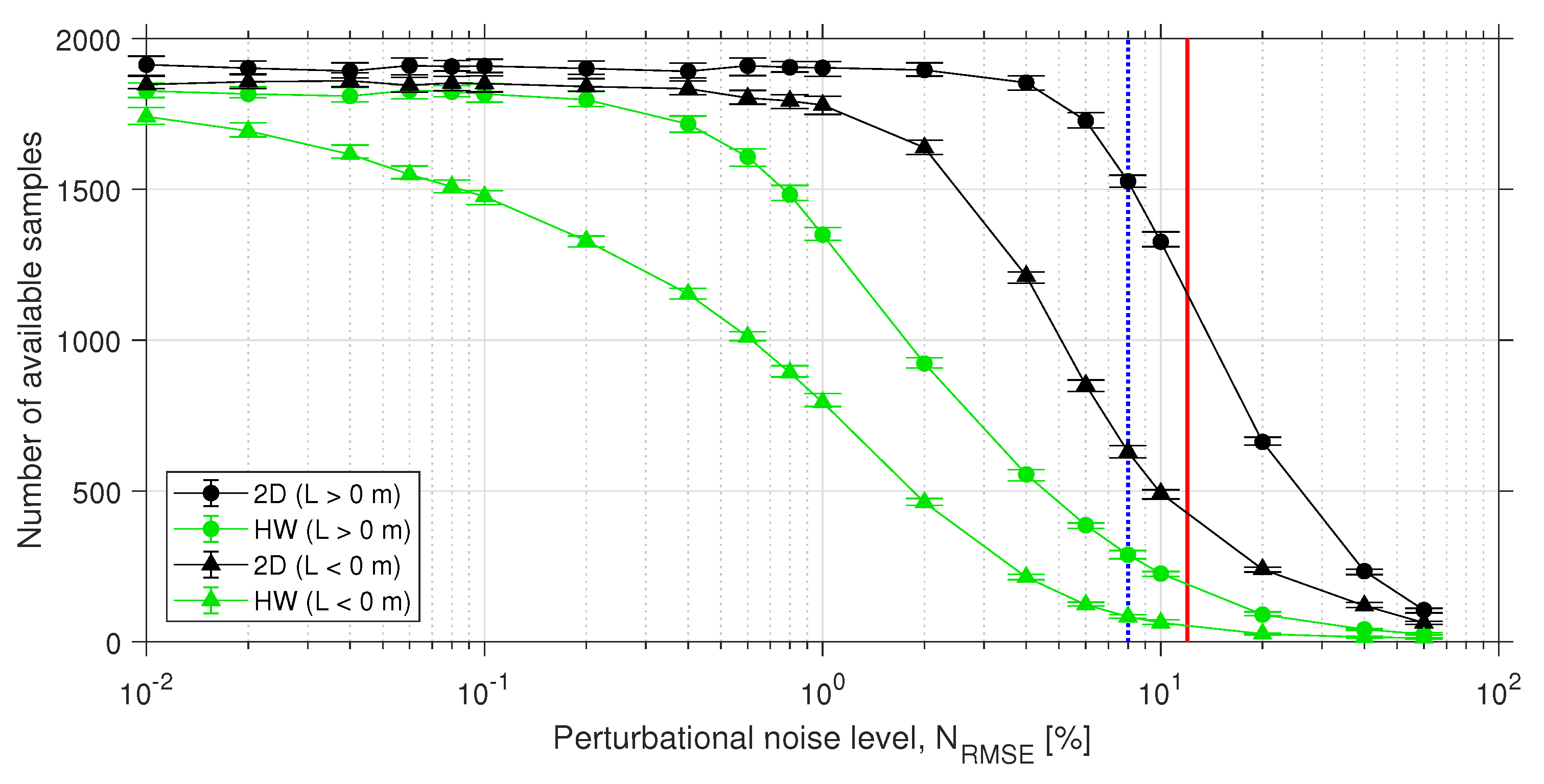
Although some authors [5,21] propose the 50 m < L < 10 m interval, our choice [35] enables symmetrical rejection of samples from the stable and unstable regimes. In addition, when the 50 m < L < 50 m rejection interval is expressed in inverse form ( | 1 / L | > 0.02 [ 1 / m]), this interval approximately corresponds to the 5th and 95th percentiles of the inverse Obukhov-length distribution, in which statistically less representative values occur (see Figure A1b). As a result from the outlier rejection criteria, the number of valid statistical samples for each dataset became smaller than the nominal simulation value of 5000. Thus, Figure 5 depicts the number of valid samples as a function of noise level N R M S E . Valid samples were counted from all the 50 datasets generated for a given perturbational noise level. For both the 2D and HW methods, the number of valid samples decreased with increasing noise level because the higher this level was, the higher the likelihood of occurrence of a non-monotonic wind profile was. Moreover, the reduction in the number of valid samples was larger for the unstable condition ( L < 0 m) on account of the fact that unstable wind profiles have lower wind shear (i.e., lower vertical wind-speed gradients) as compared to stable ones ( L > 0 m). As a result, unstable profiles are more sensitive to noise perturbations and prone to turn non-monotonic. In addition, the HW had fewer valid samples than the 2D because a larger number of HW Obukhov-length estimates fell in the outlier interval 50 m < L < 50 m.

4.2. 2D and HW Performances with Reference to Synthetic Data

4.2.1. Sensitivity to Friction Velocity

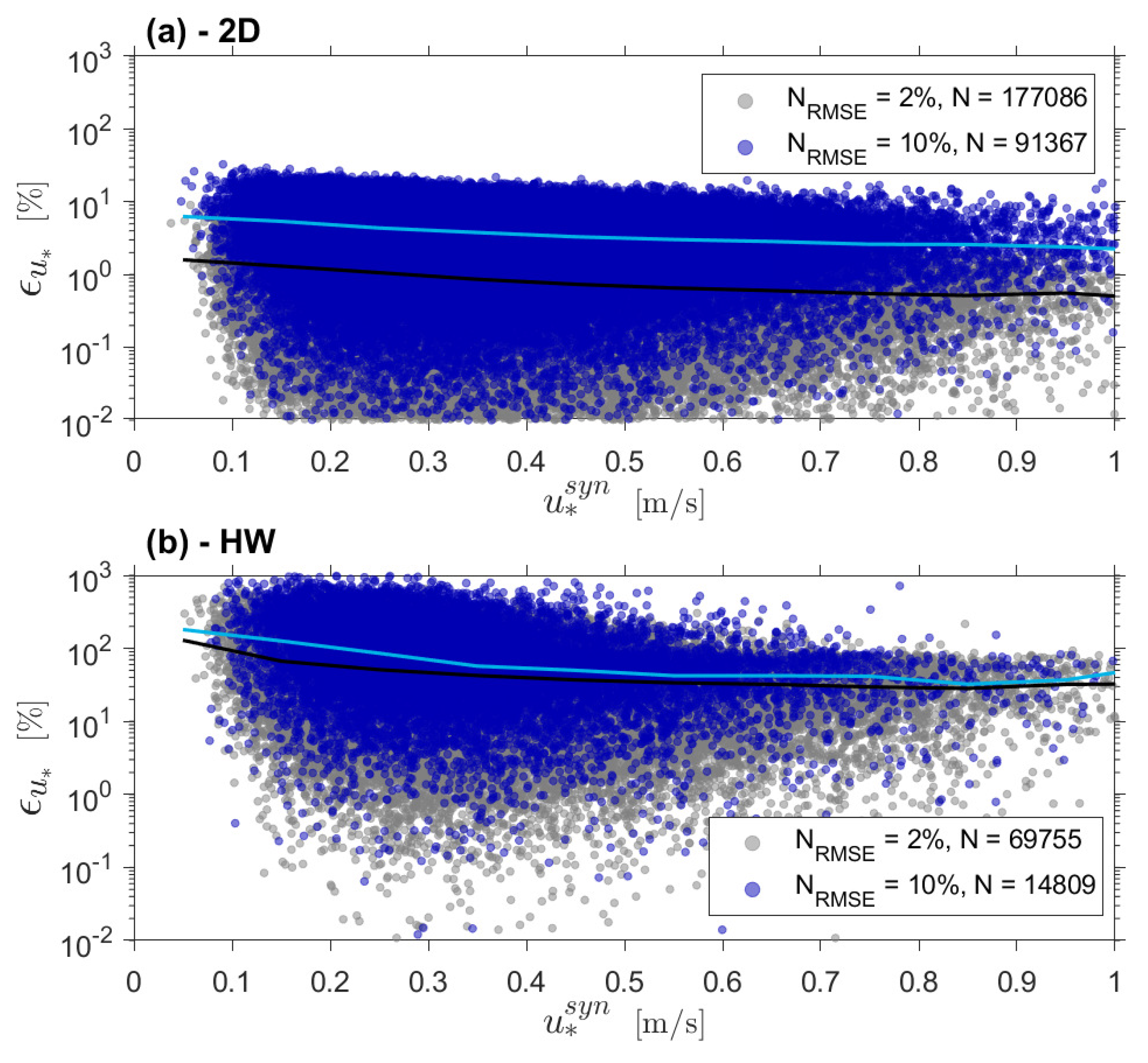
Figure 6 shows the retrieval error (Equation (19)) associated to the 2D- and HW-retrieved friction-velocity estimates ( u ^ * 2 D and u ^ * H W , respectively) as a function of reference synthetic friction velocity u * s y n for two noise levels, N R M S E = 10 % (high intensity) and N R M S E = 2 % (low). Because of the inherently stochastic nature of the perturbational noise, large dispersion in the error estimates (Equation (19)) is evidenced. To alleviate this issue, median error (50th percentile) lines are also plotted.
Prominently, it emerges that 2D retrievals consistently exhibited lower errors than HW ones for all friction velocities and noise levels. Thus, 2D estimates (Figure 6a) showed median (peak) errors of ≃ 5 %   ( 30 % ) for u * s y n = 0.1 m/s, whereas HW estimates (Figure 6b) yielded median (peak) errors as high as ≃ 200 %   ( 1000 % ) . When regarding the absolute relative error versus noise level, the higher the noise level was, the higher the error was, as expected. Comparatively, the 2D median error at N R M S E = 2 % lay between 0.5% and 1%, and at N R M S E = 10 % between 2% up to 5%, whereas the HW median error at N R M S E = 2 % and N R M S E = 10 % lay between 30% and 150%, and 40% and 200%, respectively. The worse performance of the HW is due to the fact that this algorithm does a two-step estimation: first, L is estimated from the ratio of wind speed differences (Equation (9)) and, second, u * is retrieved from the previously estimated Obukhov length (Equation (8)). As a result, the error incurred in the estimation of the Obukhov length propagates down to the friction velocity estimate. In contrast, the 2D algorithm retrieves both variables at once using a single multi-variate optimization process (Equation (10)), which does not propagate error between them.
Furthermore, for both algorithms, the error reduced with increasing friction velocity. This is in accordance with the study by Basu [15] (p. 37, Figure 4), who previously studied the sensitivity of the HW method to friction velocity under four different noise cases. In that study, case-4 scenario consisted of a multivariate Gaussian noise distribution with standard deviation σ = 0.05 m/s and the assumption of noise-correlated heights with correlation coefficient ρ = 0.5 . That standard deviation ( σ = 0.05 m/s) is equivalent to our noise level N R M S E = 2 % representing HWS deviations from MOST up to ± 0.2 m/s. Quantitative results are as follows: On one hand, Figure 4 in Basu [15] reported median errors between ≈50% and 8% for friction velocities between 0.1 and 1 m/s. On the other hand, we found (Figure 6b) that the HW method attained median errors between 150% and 30% for N R M S E = 2 % within the same range of friction velocities. Therefore, both Basu [15] and our study yield similar quantitative results, albeit a factor three higher error in our simulations due to the conservative assumption of uncorrelated noise.

4.2.2. Sensitivity to the Perturbational Noise Level

Numerical analysis was used to assess 2D and HW algorithm performances for friction velocity, Obukhov length, and heat flux estimation. Towards this purpose, both algorithms computed these three parameters from each of the 50 datasets generated for each noise level (Section 4.1). The coefficient of determination ( ρ 2 ) enabled us to calculate the degree of correlation between each of the estimated parameters and their corresponding synthetic reference in each dataset. As a result, for each parameter and noise level a set of 50 coefficients of determination was obtained.
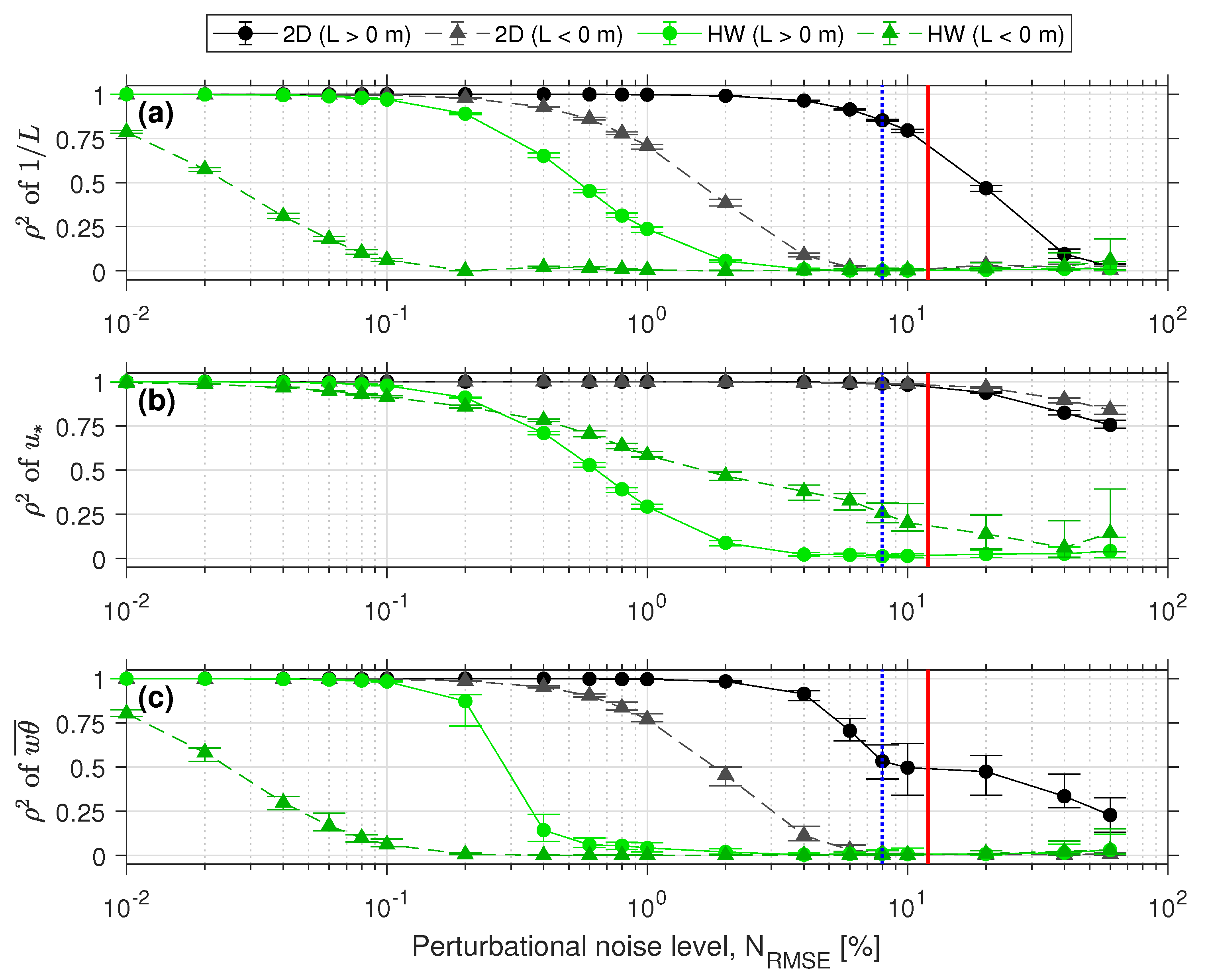
Figure 7 shows ρ 2 as function of noise level for the three parameters above. It can be observed that both the 2D and HW algorithms exhibited ideal performance ( ρ 2 = 1 ) in the absence of noise ( N R M S E 0 ) for all three parameters. As expected, the coefficients of determination decreased with increasing noise, being the 2D method more robust to noise perturbations as shown by ρ 2 values higher than those from the HW algorithm.
Friction velocity (Figure 7b) became the least sensitive parameter to noise as evidenced by much higher coefficients of determination than those obtained for the Obukhov length and heat flux. This is because friction velocity is proportional to the mean wind speed. As found in Section 4.2.1, 2D friction-velocity estimates were more accurate than HW ones. Thus, the 2D method yielded coefficients of determination ρ 2 > 0.75 for all simulated noise levels, whereas the HW dropped below 0.5 for noise levels higher than N R M S E = 5 % . Two-dimensional friction-velocity estimates were unaffected by atmospheric stability, as evidenced by the stable-condition trace ( L > 0 m, black solid) overlapping the unstable one ( L < 0 m, grey dashed). On the other hand, HW friction-velocity exhibited higher performances in unstable conditions.
With regards to the Obukhov length (actually to its inverse 1 / L , Figure 7a), the 2D algorithm was able to acceptably estimate of the Obukhov length in stable regimes ( L > 0 m), yielding ρ 2 0.8 at N R M S E = 8 % (which is the mean noise level, N R M S E , found during the IJmuiden campaign, Figure 4d). At this same noise level, the HW method showed ρ 2 0 . The higher accuracy of the 2D algorithm in stable conditions was already reported by Araújo da Silva et al. [5]. On the other hand, none of the methods was able to successfully estimate the Obukhov length in unstable conditions ( L < 0 m). Quantitatively, ρ 2 values were virtually zero for N R M S E > 4 % .
As far as the heat flux is concerned (Figure 7c), the coefficients of determination obtained were similar to those for the Obukhov length in Figure 7a, because the heat flux is a secondary parameter derived from u * and L through Equation (7). ρ 2 values were slightly higher for the Obukhov length than for the heat-flux retrievals when using the 2D algorithm, particularly, for high noise levels ( N R M S E > 5 % ). A suitable explanation for that is propagation of the Obukhov-length estimation error to heat-flux estimates via Equation (7).

4.3. 2D- and HW-Algorithm Performances with Reference to Observational Data

Performance of the two surface-layer retrieval algorithms was also evaluated with reference to metmast observational data gathered during the IJmuiden campaign (Section 2). A total of 8263 10-min FDWL-measured wind profiles were used as the sole input for the 2D and HW methods after prior removal of high spatial-variation data, and HWS values outside the range 2–80 m/s (refer to [5] for detailed FDWL outlier-filtering procedure). We verified that the coefficients of determination were higher than ρ 2 = 0.996 between the FDWL and anemometer measurements for the three metmast reference heights closest to the lidar (27, 58.5 and 85 m Section 2). After this verification step, the observational data collection was submitted to the same outlier rejection criteria as the ones applied over synthetic data (Section 4.1.1).
The first part of our analysis consisted of testing the capabilities of the 2D and HW algorithms for typing the observational wind profiles into three main atmospheric stability classes (Table 1) [35,36]: unstable (u), neutral (n), and stable (s). The L values used for the classification were the corresponding 2D- and HW-retrieved Obukhov lengths, denoted L 2 D and L H W , respectively.
Figure 8 plots the measured median normalized wind-speed profiles (normalized the wind speed at the lowest height, U ( z 1 ) ) for cluster categories u, n, and s derived from the 2D- and HW-retrieved Obukhov lengths ( L 2 D and L H W , respectively) over the whole campaign. As observed, both 2D and HW algorithms were able to discern among the different stability types. The 2D algorithm enabled clearer discrimination among the three stability types and showed narrower non-overlapping error bars as compared to the HW. Further, the median wind-speed profiles in Figure 8 (i.e., he profiles resulting from computing the median speed at each measuring height of the lidar and for each stability class) follow MOST. This is also in agreement with the results found by other authors who also used MOST (e.g., Figure 4 in [21] and Figure 3 in [33]). For the 2D algorithm the behaviour of the wind shear is clearly different for the number of stability classes.
The second part of our analysis tackled numerical evaluation of the 2D and HW retrieval performances through direct comparison with reference metmast retrievals. The Richardson-number-based Obukhov-length, L R i (Appendix A), numerically-solved friction velocity, u * 1 D (see Section 3.3), and heat flux, w θ ¯ , computed through Equation (7) using L R i and u * 1 D , were the references used in this study (Section 3.3).
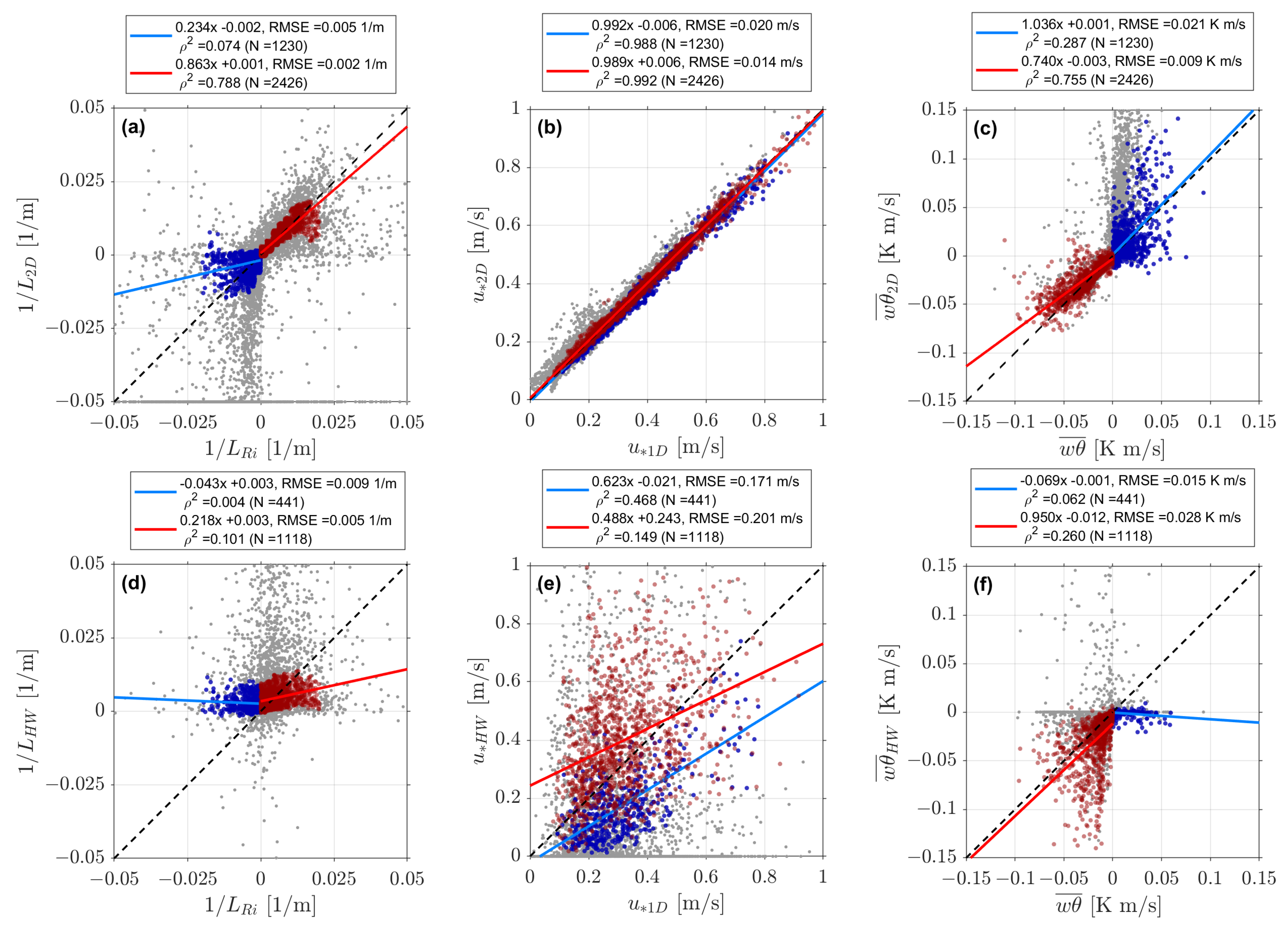
Scatter plots comparing 2D- and HW-retrievals to the mast-derived reference estimates are shown in Figure 9. Aimed at limiting linear regression (LR) analysis to the most meaningful samples, an additional de-noising filtering procedure named histogrammed filtering was applied as follows: the range for X-axis data (reference reciprocal-Obukhov-length range, 0.05 [ 1 / m ] < 1 / L R i < 0.05 [ 1 / m ] ) in Figure 9a,d was divided into 0.002 [1/m]-width bins and, in each bin, the corresponding Y-values (estimated reciprocal-Obukhov-length values 1 / L 2 D in Figure 9a, or 1 / L H W in Figure 9d) outside the 15th-to-85th-percentile interval were rejected as outliers, therefore, excluded from the LR. At this point we note that the 15th-to-85th percentile is approximately one standard deviation of the mean in a normal distribution. For consistency, rejected samples in the Obukhov-length estimates (grey dots in Figure 9a,d) were also rejected in the friction-velocity and heat-flux estimates (Figure 9b,c and Figure 9e,f, respectively).
After histogrammed filtering, the 2D method remained with N = 2426 and N = 1230 samples for the stable ( 1 / L 2 D > 0 [ 1 / m ] ) and unstable ( 1 / L 2 D < 0 [ 1 / m ] ) classes, respectively (see legends in Figure 9) whereas the HW remained with 1118 ( 1 / L H W > 0 [ 1 / m ] ) and 441 ( 1 / L H W < 0 [ 1 / m ] ) samples, respectively. Overall, the results of Figure 9 agree with those previously found in Figure 7 using synthetic data and show that the 2D outperforms the HW algorithm. Thus, the 2D-derived friction velocity, u * 2 D , outperformed all other retrievals regardless of the atmospheric stability condition (Figure 9b using observational data and Figure 7b using synthetic data), and the HW-estimated friction velocity, u * H W , yielded coefficients of determination ρ 2 = 0.47 and 0.15 ( ρ 2 = 0.39 and 0.12 without histogrammed filtering) for unstable and stable cases (Figure 9e) in rough agreement with the 1D friction velocity results of Figure 7b, in which coefficients ρ 2 = 0.25 –0 were respectively found at N R M S E = 8 % (the observational median noise level, Figure 4d).
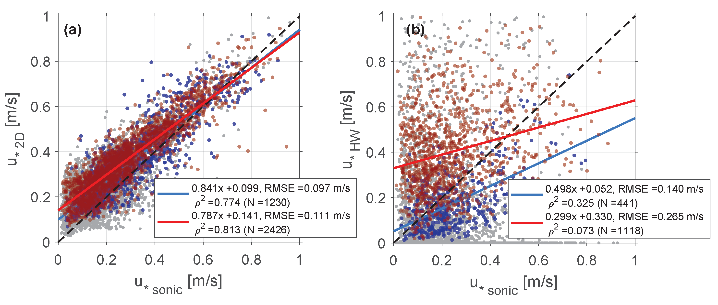
Finally, in the third part of our study we compared the 2D and HW friction-velocity estimates ( u * 2 D and u * H W ) against the corresponding sonic-anemometer measurements ( u * s o n i c ), Figure 10. For consistency, histogrammed outliers identified in Figure 9a,d were also excluded in Figure 10. Similar to the results found in Section 4.2, the 2D algorithm attained the best numerical indicators in both the stable and unstable atmospheric regimes, whereas the HW algorithm could only assess the friction velocity in the unstable one. Without histogrammed filtering, the HW-retrieved friction velocity results yielded coefficients of determination of ρ 2 = 0.26 and ρ 2 = 0.1 for the unstable and stable types, respectively, which are virtually the same results as those found with synthetic data at 8% noise level (observational median noise level) in Figure 7b ( ρ 2 = 0.25 and ρ 2 = 0.0 , respectively). Note that u * s o n i c is the local friction velocity at 85 m, which might be different from the surface-layer value (Section 3.3). Therefore, reference sonic-anemometer retrievals closer to the surface would be necessary to increase the validity of our findings.

5. Conclusions

Two retrieval algorithms aimed at estimating surface-layer parameters from solely wind profiles, namely, the 2D and the Hybrid-Wind methods, were compared. Their performances for estimating the Obukhov length, friction velocity and heat flux were assessed by means of synthetic data and observational data gathered at the IJmuiden meteorological site.
In order to assess 2D and HW performances with reference to synthetic data, a method to computationally generate surface-layer parameters was devised. By modelling the so-called c-factor (i.e., the proportionality factor between the Obukhov length and the cube of the friction velocity, Equation (12)) and the friction velocity as random variables with log-normal-like PDFs, statistically meaningful Obukhov-length and friction-velocity pairs were reproduced (Figure A1). Synthetic noisy wind profiles were generated from these pairs via MOST and the addition of Gaussian perturbational noise to the theoretical MOST profiles. For algorithm intercomparison, 5,000,000 synthetic wind profiles with 20 noise levels ranging from N R M S E 0.01 % to N R M S E = 60 % were generated.
As for the assessment of 2D and HW performances with reference to observational data, FDWL-measured wind profiles were used as the only input to the algorithms. Reference parameters were retrieved from the metmast instrumentation (Section 3.3).
Retrieval performance of the 2D and HW methods as a function of the noise level was studied by using both synthetic and observational data. It was found that:
(i) Regarding synthetic data, performance results obtained are summarised in Figure 6 and Figure 7. For noise-free synthetic profiles ( N R M S E 0 ), the 2D and the HW performed equally. Out of this idealised condition, 2D and HW friction-velocity retrievals were more accurate than Obukhov-length and heat-flux ones (Figure 7). Moreover, neither the 2D nor the HW were able to satisfactorily estimate the Obukhov length (L) or the kinematic heat flux ( ω θ ¯ ) in unstable regimes (Figure 7a,c). Conversely, under stable conditions, the 2D was the only method able to retrieve meaningful Obukhov-length and heat-flux estimates. Overall, the 2D outperformed the HW for the three surface-layer parameters considered.
From a numerical perspective, the smaller errors obtained in the retrieval of the friction velocity by both algorithms (Figure 2) are due to the fact that the MOST model (Equation (1)) is very sensitive to the friction velocity. Concerning the HW, there are two key reasons accounting for its poorer performance: First, the HW is a two-step processing algorithm itself, in which a variable Obukhov length is first estimated and, subsequently, a variable friction velocity from the previous Obukhov-length estimate, hence propagating errors. Second, the HW algorithm relies on the MOST assumption of nearly constant momentum and heat fluxes within the surface layer [13], which is used to compute the ratio of the wind-speed differences and, eventually, to estimate the Obukhov length from this ratio (Equation (9)). Instead, the 2D algorithm directly fits the MOST wind-profile model to the measured profile, which is equivalent to extrapolating the model up to the highest measurement height.
(ii) Regarding cross-examination with observational data, Figure 9 and Figure 10 were in agreement with the results derived from synthetic data (Figure 7), hence validating the representativeness of the latter. Thus, at N R M S E = 8 % , which was the observational median noise level in IJmuiden campaign, 2D friction-velocity retrievals from either observational or synthetic data showed ρ 2 > 0.9 under stable and unstable atmospheric conditions (Figure 7b). In contrast, HW friction-velocity retrievals from observational data yielded coefficients of determination of ρ 2 = 0.1 (stable) and ρ 2 = 0.26 (unstable) [ ρ 2 = 0.15 (s) and ρ 2 = 0.47 (u) with histogrammed filtering, Figure 9e] versus ρ 2 = 0.0 (s) and ρ 2 = 0.25 (u) from synthetic data (Figure 7b). As for the Obukhov-length and heat-flux estimates, the 2D was the only method able to achieve acceptable performance in stable regimes ( ρ 2 0.8 ). Furthermore, the 2D also prevailed over the HW when comparing their estimates against reference sonic anemometer measurements or derived Richardson-number approximations (Appendix A) from the sonics (Figure 10 and Figure 9, respectively).
When addressing 2D and HW atmospheric stability typing performance, our results are two-fold: On the long time scale (82-day average, i.e., the IJmuiden campaign duration) observational data showed that both methods output similar median wind-speed profiles for each stability class (Figure 8), the 2D exhibiting narrower error bars. On the short time scale (10-min estimates), observational data (Figure 9a) showed that the 2D method was the only one able to achieve acceptable performance in stable regimes (see point (ii) above).
As far as data availability is concerned, it is important to highlight that the 2D method can fit a lidar wind profile with any number of measurement heights whereas the HW is limited to about three. Because of MOST implicit assumption that wind speeds monotonically increase with height, the larger the number of heights, the more likely measurement samples break the monotonicity requirement, therefore, risking to run out of valid MOST-compliant samples.
All in all, we highlight the 2D algorithm as an attractive method for estimating the Obukhov length, friction velocity and turbulent fluxes utilizing only wind-speed profile measurements in and close to the surface layer (25 to 85 m in this work). As further steps, comparisons against momentum and heat flux at lower altitudes (i.e., below 25 m) would be advisable.

Author Contributions

This work was developed as part of M.P.A.d.S.’s doctoral thesis supervised by F.R.; 2D optimization algorithm methodology, F.R. and M.P.A.d.S.; software development, A.S.-B. and M.P.A.d.S.; analysis and figures, M.P.A.d.S. and A.S.-B.; writing—original draft preparation, M.P.A.d.S. and A.S.-B.; review and editing, F.R. and A.P.; funding acquisition, F.R.; conceptualization support, F.R. and A.P. All authors have read and agreed to the published version of the manuscript.

Funding

This research is part of the project PID2021-126436OB-C21 funded by Ministerio de Ciencia e Investigación (MCIN)/Agencia Estatal de Investigación (AEI)/10.13039/501100011033 y FEDER “Una manera de hacer Europa”. The work of M.P Araújo da Silva was supported under Grant PRE2018-086054 funded by MCIN/AEI/10.13039/501100011033 and FSE “El FSE invierte en tu futuro”. The work of A. Salcedo-Bosch was supported under grant 2020 FISDU 00455 funded by Generalitat de Catalunya—AGAUR. The European Commission collaborated under projects H2020 ATMO-ACCESS (GA-101008004) and H2020 ACTRIS-IMP (GA-871115).

Data Availability Statement

The data presented in this study are available upon request from the corresponding author, [email protected].

Acknowledgments

Profs. A. Peña and J. Mann (Denmark Technical University, DTU) are gratefully acknowledged for hosting M. P. Araújo da Silva and A. Salcedo-Bosch during their Ph.D. secondments to DTU. Prof. Sukanta Basu (Atmospheric Sciences Research Center, University at Albany, SUNY) is kindly acknowledged for his insightful technical assistance.

Conflicts of Interest

The authors declare no conflict of interest.

Abbreviations

The following abbreviations are used in this manuscript:
1DOne-dimensional
2DTwo-dimensional
ABLAtmospheric boundary layer
ABLHABL height
DWLDoppler wind lidar
FDWLFloating Doppler wind lidar
HWHybrid Wind
HWSHorizontal wind speed
MOSTMonin–Obukhov similarity theory
N R M S E Normalised root-mean-squared error
PDFProbability density function
RMSERoot-mean-squared error

Appendix A. Derivation of Obukhov Length from Richardson Number

The bulk-Richardson number approximates local gradients in an atmospheric layer by means of measurements at different discrete heights. The bulk-Richardson number is defined as [13]
R i = g Δ θ ¯ v Δ z θ ¯ v Δ U 2 , z [ z b o t t o m , z t o p ] ,
where Δ z = z t o p z b o t t o m is the difference between the top layer height, z t o p , and the bottom layer height, z b o t t o m , and Δ θ ¯ v = θ ¯ v ( z t o p ) θ ¯ v ( z b o t t o m ) is the mean virtual potential temperature difference between z t o p and z b o t t o m . θ ¯ v is the mean virtual potential temperature within the layer and Δ U = U ( z t o p ) U ( z b o t t o m ) is the HWS difference between the 10-min mean HWS measured at z t o p and z b o t t o m .
The virtual potential temperature can be estimated as [13]
θ v ( z ) = T ( z ) P 0 P ( z ) R C p [ 1 + 0.61 r ( z ) ] ,
where T [K] is the temperature, P 0 = 1000 hPa is the pressure at the sea surface, P is the measured air pressure, R 287 J/(K·kg) is the gas constant of air, C p 1004 J/(K·kg) is the specific heat capacity at a constant pressure for air, and r is the mixing ratio. The mixing ratio was computed via Equations (4.1a), (4.4) and (4.14a), pp. 88, 91–92 [7].
From the bulk-Richardson number, the dimensionless stability parameter ζ = z / L can be computed as
ζ = 10 R i R i 0 10 R i 1 5 R i 0 < R i < 0.2 .
Finally, the Obukhov length can be derived from the dimensionless stability as
L R i ( z ) = z ζ ,
where z is a reference height ensuring the validity of the bulk-Richardson model within the layer [ z b o t t o m , z t o p ] .
Here, we follow the same procedure as in [5] to derive the Obukhov length from the bulk-Richardson number. We consider z t o p = 21 m and z b o t t o m = 0 m above the Lowest Astronomical Tide (LAT). U ( z t o p ) is measured by the metmast anemometers at 21 m above LAT (see Section 2) and U ( z b o t t o m ) = 0 m/s is assumed. Regarding the virtual potential temperature, θ v ¯ ( z t o p ) is obtained from the mast temperature, pressure, and humidity sensors at 21 m. θ v ¯ ( z b o t t o m ) is computed from the wave-buoy-measured water temperature, and the pressure and relative humidity at z b o t t o m = 0 m are extrapolated from the mast pressure and humidity profiles measured by the sensors at 90 m and 21 m down to 0 m. Reference height z in Equation (A4) is taken as z = 15.5 m (refer to [5] for further details).

Appendix B. Quality Assurance of “Seed” PDF Characteristic Parameters
For the IJmuiden campaign, friction velocity PDFs parameters of μ u * = 1.36 and σ u * = 0.52 were obtained. Analogously, μ C , p = 10.29 and σ C , p = 0.52 , and μ C , n = 10.96 and σ C , n = 1.11 parameters were obtained for the C-factor PDF.
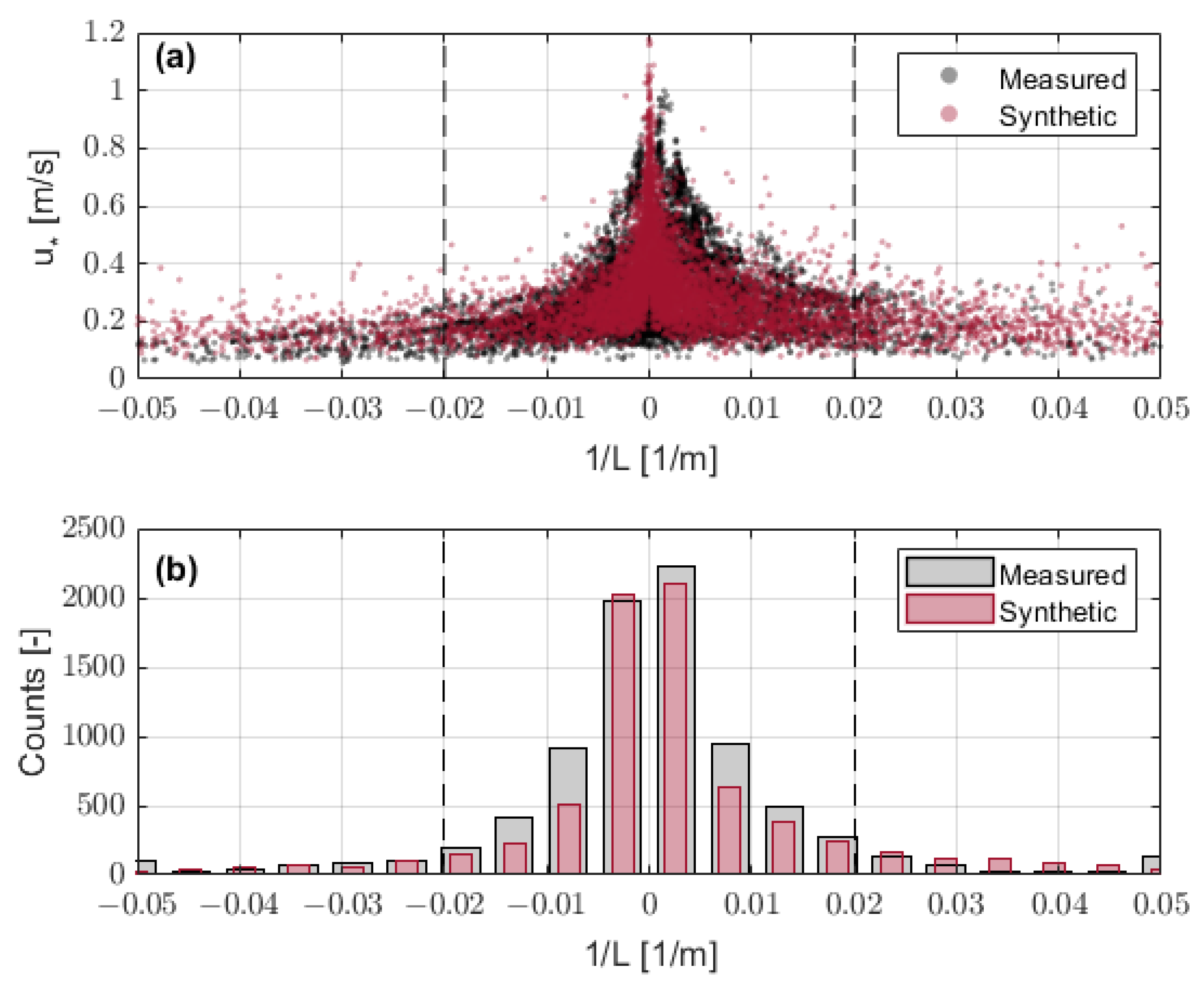
Concerning quality assurance, in order to ensure trustworthy synthetic datasets in comparison to the observational ones gathered at IJmuiden, we generated 8263  ( u * s y n , L s y n ) pairs and compared the u * s y n -to- 1 / L s y n (i.e., the friction-velocity-to-reciprocal-Obukhov-length) distribution to the u * s o n i c -to- 1 / L R i distribution measured at IJmuiden. The outcome of this exercise is depicted in Figure A1. As can be observed in Figure A1a, the distribution of the synthetic pairs (red dots) virtually overlaps that of the measured pairs (black dots), which validates the synthetic generation method described in Section 3.4.2. In addition, Figure A1b shows the histogram of the reciprocal of the Obukhov length distribution for both the synthetic and measured datasets, which are virtually identical.
Figure A1. Synthetic data quality assurance. (a) Comparison between synthetic (red dots) and measured (black dots) distributions of friction-velocity and Obukhov-length as ( u * s y n , 1 / L s y n ) pairs. (b) Obukhov-length histograms for the measured and synthetic pairs. X-axis plots reciprocal Obukhov length in 0.005 m 1 -width bins. (Dashed vertical lines) Outlier-rejection interval bounds, ( 0.02 < 1 / L < 0.02 ) 1/m.
Remotesensing 15 02660 g0a1

References

  1. GWEC. Global Wind Report 2022; Technical Report; Global Wind Energy Council: Brussels, Belgium, 2022. [Google Scholar]
  2. Hevia-Koch, P.; Jacobsen, H.K. Comparing offshore and onshore wind development considering acceptance costs. Energy Policy 2019, 125, 9–19. [Google Scholar] [CrossRef]
  3. WindEurope. Offshore Wind in Europe Key Trends and Statistics 2019; Technical Report; WindEurope: Brussels, Belgium, 2020. [Google Scholar]
  4. Peña, A.; Mann, J.; Angelou, N.; Jacobsen, A. A Motion-Correction Method for Turbulence Estimates from Floating Lidars. Remote Sens. 2022, 14, 6065. [Google Scholar] [CrossRef]
  5. Araújo da Silva, M.P.; Rocadenbosch, F.; Farré-Guarné, J.; Salcedo-Bosch, A.; González-Marco, D.; Peña, A. Assessing Obukhov Length and Friction Velocity from Floating lidar Observations: A Data Screening and Sensitivity Computation Approach. Remote Sens. 2022, 14, 1394. [Google Scholar] [CrossRef]
  6. Gutiérrez-Antuñano, M.A.; Tiana-Alsina, J.; Rocadenbosch, F. Performance evaluation of a floating lidar buoy in nearshore conditions. Wind Energy 2017, 20, 1711–1726. [Google Scholar] [CrossRef]
  7. Stull, R.B. Practical Meteorology: An Algebra-Based Survey of Atmospheric Science; University of British Columbia: Kelowna, BC, USA, 2015. [Google Scholar]
  8. Holtslag, M.C.; Bierbooms, W.A.A.M.; Van Bussel, G.J.W. Validation of surface layer similarity theory to describe far offshore marine conditions in the Dutch North Sea in scope of wind energy research. J. Wind Eng. Ind. Aerodyn. 2015, 136, 180–191. [Google Scholar] [CrossRef]
  9. Türk, M.; Emeis, S. The dependence of offshore turbulence intensity on wind speed. J. Wind Eng. Ind. Aerodyn. 2010, 98, 466–471. [Google Scholar] [CrossRef]
  10. Göçmen, T.; Van der Laan, P.; Réthoré, P.E.; Diaz, A.P.; Larsen, G.C.; Ott, S. Wind turbine wake models developed at the technical university of Denmark: A review. Renew. Sustain. Energy Rev. 2016, 60, 752–769. [Google Scholar] [CrossRef]
  11. Lopez-Villalobos, C.; Martínez-Alvarado, O.; Rodriguez-Hernandez, O.; Romero-Centeno, R. Analysis of the influence of the wind speed profile on wind power production. Energy Rep. 2022, 8, 8079–8092. [Google Scholar] [CrossRef]
  12. Gao, Z.; Qian, X.; Wang, T. Spectral partition characteristics of wind turbine load response under different atmospheric stability. Sustain. Energy Technol. Assess. 2021, 47, 101421. [Google Scholar] [CrossRef]
  13. Stull, R.B. An Introduction to Boundary Layer Meteorology; Kluwer Academic Publishers: Amsterdam, The Netherlands, 1988. [Google Scholar]
  14. Grachev, A.; Fairall, C. Dependence of the Monin–Obukhov stability parameter on the bulk Richardson number over the ocean. J. Appl. Meteorol. 1997, 36, 406–414. [Google Scholar]
  15. Basu, S. Hybrid profile–gradient approaches for the estimation of surface fluxes. Bound. Layer Meteorol. 2019, 170, 29–44. [Google Scholar] [CrossRef] [PubMed]
  16. Berkowicz, R.; Prahm, L.P. Evaluation of the profile method for estimation of surface fluxes of momentum and heat. Atmos. Environ. 1982, 16, 2809–2819. [Google Scholar] [CrossRef]
  17. Klug, W. Determination of turbulent fluxes of heat and momentum from the wind profile. Q. J. R. Meteorol. Soc. 1967, 93, 101–104. [Google Scholar] [CrossRef]
  18. Swinbank, W. The exponential wind profile. Q. J. R. Meteorol. Soc. 1964, 90, 119–135. [Google Scholar] [CrossRef]
  19. Lo, A.K. On the determination of boundary-layer parameters using velocity profile as the sole information. Bound. Layer Meteorol. 1979, 17, 465–484. [Google Scholar] [CrossRef]
  20. Beljaars, A.C.M.; Holtslag, A.; Van Westrhenen, R. Description of a Software Library for the Calculation of Surface Fluxes; KNMI De Bilt: Utrecht, The Netherlands, 1989. [Google Scholar]
  21. Gryning, S.E.; Batchvarova, E.; Brümmer, B.; Jørgensen, H.; Larsen, S. On the extension of the wind profile over homogeneous terrain beyond the surface boundary layer. Bound. Layer Meteorol. 2007, 124, 251–268. [Google Scholar] [CrossRef]
  22. Jiang, Q.; Sullivan, P.; Wang, S.; Doyle, J.; Vincent, L. Impact of swell on air–sea momentum flux and marine boundary layer under low-wind conditions. J. Atmos. Sci. 2016, 73, 2683–2697. [Google Scholar] [CrossRef]
  23. Chen, S.; Qiao, F.; Jiang, W.; Guo, J.; Dai, D. Impact of surface waves on wind stress under low to moderate wind conditions. J. Phys. Oceanogr. 2019, 49, 2017–2028. [Google Scholar] [CrossRef]
  24. Jiang, Q. Influence of swell on marine surface-layer structure. J. Atmos. Sci. 2020, 77, 1865–1885. [Google Scholar] [CrossRef]
  25. Zhang, S.F. Comments on ‘on the determination of boundary-layer parameters using velocity profile as the sole information’ by LO (1979). Bound. Layer Meteorol. 1981, 21, 127–129. [Google Scholar] [CrossRef]
  26. Businger, J.A.; Wyngaard, J.C.; Izumi, Y.; Bradley, E.F. Flux-profile relationships in the atmospheric surface layer. J. Atmos. Sci. 1971, 28, 181–189. [Google Scholar] [CrossRef]
  27. Dyer, A.J. A review of flux-profile relationships. Bound. Layer Meteorol. 1974, 7, 363–372. [Google Scholar] [CrossRef]
  28. Peña, A.; Hasager, C.B.; Gryning, S.E.; Courtney, M.; Antoniou, I.; Mikkelsen, T. Offshore Wind Profiling Using Light Detection and Ranging Measurements. Wind Energy 2009, 12, 105–124. [Google Scholar] [CrossRef]
  29. Barthelmie, R. The effects of atmospheric stability on coastal wind climates. Meteorol. Appl. A J. Forecast. Pract. Appl. Train. Tech. Model. 1999, 6, 39–47. [Google Scholar] [CrossRef]
  30. Högström, U. Non-dimensional wind and temperature profiles in the atmospheric surface layer: A re-evaluation. In Topics in Micrometeorology. A Festschrift for Arch Dyer; Springer: Berlin/Heidelberg, Germany, 1988; pp. 55–78. [Google Scholar]
  31. Charnock, H. Wind stress on a water surface. Q. J. R. Meteorol. Soc. 1955, 81, 639–640. [Google Scholar] [CrossRef]
  32. Peña, A.; Gryning, S.E. Charnock’s roughness length model and non-dimensional wind profiles over the sea. Bound. Layer Meteorol. 2008, 128, 191–203. [Google Scholar] [CrossRef]
  33. Basu, S. A simple recipe for estimating atmospheric stability solely based on surface-layer wind speed profile. Wind Energy 2018, 21, 937–941. [Google Scholar] [CrossRef]
  34. Devroye, L. Non-Uniform Random Variate Generation; Springer: New York, NY, USA, 2013. [Google Scholar]
  35. Kretschmer, M.; Schwede, F.; Guzmán, R.F.; Lott, S.; Cheng, P.W. Influence of atmospheric stability on the load spectra of wind turbines at alpha ventus. J. Phys. 2018, 1037, 052009. [Google Scholar] [CrossRef]
  36. Araújo da Silva, M.P.; Rocadenbosch, F.; Farré-Guarné, J.; Salcedo-Bosch, A.; González-Marco, D.; Peña, A. Floating Lidar Assessment of Atmospheric Stability in the North Sea. In Proceedings of the IGARSS 2022—2022 IEEE International Geoscience and Remote Sensing Symposium, Kuala Lumpur, Malaysia, 17–22 July 2022; pp. 7313–7316. [Google Scholar]
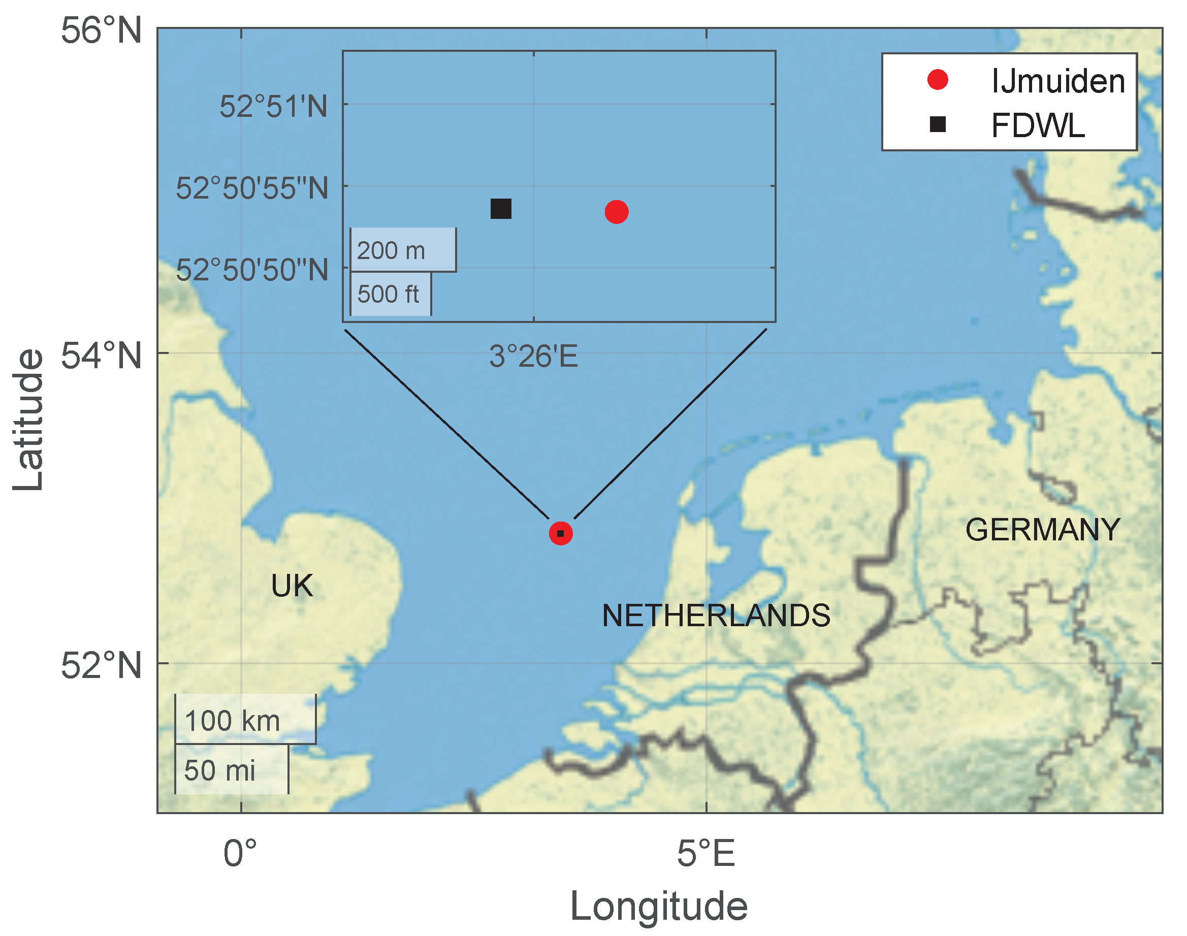
Figure 1. Map showing the locations of the IJmuiden metmast in the North sea. The zoom plot in the upper part of the map shows the FDWL location at IJmuiden.
Remotesensing 15 02660 g001
Figure 2. MOST wind profiles (Equation (1)) and numerical sensitivity. (a) MOST model for different stability conditions. (u) is unstable, (n) is neutral and (s) is stable. (b) Sensitivity to the friction velocity, u * . (c) Sensitivity to the Obukhov length, L. (All panels) Simulation parameters: z 0 = 0.01 m, u * = 0.45 m/s and L = 200 , 10 , 000 , and 200 m (see legends). Error bars computed by applying a 10 % perturbation to the nominal value of the variable under study.
Remotesensing 15 02660 g002
Figure 3. Block diagram summarising the procedure to generate synthetic pairs ( u * s y n , L s y n ) and corresponding noise-corrupted wind profiles, U s y n ( z ) .
Remotesensing 15 02660 g003
Figure 4. Estimation of normalised noise level N R M S E from metmast observations. (ac) Comparison between the MOST-predicted (Equation (1)) and mast-measured wind speed at the three measurement heights. Dashed green line is the ideal 1:1 line. Red line is the linear regression line. (d) Distribution of normalised noise level N R M S E (Equation (17)), computed between predicted and reference wind-speed profiles for the whole observational campaign.
Remotesensing 15 02660 g004
Figure 5. Distribution of the number of valid samples (i.e., after rejecting outliers) from all 50 datasets for a given noise level as a function of perturbational noise level N R M S E (Equation (17)). Symbols indicate median levels. Lower and upper error bars depict 25th and 75th percentiles, respectively. Blue and red lines respectively correspond to the median (8%) and mean (12%) noise levels shown in Figure 4d.
Remotesensing 15 02660 g005
Figure 6. Absolute relative error between the estimated and reference synthetic friction velocity (Equation (19)) for two different noise levels (see legends). (a) 2D method. (b) HW method. (Blue trace) Median error at noise level N R M S E = 2 % . (Black trace) Median error at N R M S E = 10 % . N stands for number of samples.
Remotesensing 15 02660 g006
Figure 7. Performance statistics as a function of perturbational noise level N R M S E . (a) Inverse of Obukhov length, 1 / L . (b) Friction velocity, u * . (c) Kinematic heat flux, w θ ¯ . Symbols and error bars: Same format as in Figure 5. ρ 2 is the coefficient of determination.
Remotesensing 15 02660 g007
Figure 8. (Observational data, Section 4.3, part I) 2D and HW atmospheric stability typing performance (82-day time resolution): median wind-speed profiles measured by the FDWL during IJmuiden campaign clustered by stability classes (Table 1). Panels (a) and (b) show classifications based on the 2D- and HW-retrieved Obukhov lengths, L 2 D and L H W , respectively. (u) stands for unstable, (n) for neutral and (s) for stable. Error bars depict 40th-to-60th percentiles at each height (note that median is the 50th percentile in the very middle of the error bar).
Remotesensing 15 02660 g008
Figure 9. (Observational data, Section 4.3, part II) 2D and HW quantitative retrieval performances (10 min resolution): estimated reciprocal Obukhov length, friction velocity and heat flux against reference metmast retrievals. (ac) 2D-algorithm performance. (df) HW-algorithm performance. (Red and blue dots) Colour-coded reference Obukhov length as 1 / L R i > 0 [ 1 / m ] and 1 / L R i < 0 [ 1 / m ] , respectively. (Red and blue lines) Corresponding regression lines. (Black-dashed line) 1:1 ideal reference line. (Grey dots) Outlier samples. ρ 2 is the coefficient of determination. N stands for number of samples used in the linear regression. R M S E stands for root-mean-squared error.
Remotesensing 15 02660 g009
Figure 10. (Observational data, Section 4.3, part III) 2D and HW friction-velocity estimates versus reference sonic-anemometer ones (10 min resolution, Equation (11)). (a) 2D estimates. (b) HW estimates. Same format as in Figure 9.
Remotesensing 15 02660 g010
Table 1. Relationship between atmospheric stability classes and the Obukhov length (refer to Section 4.1.1 (ii)).
CategoryL Range [m]
Stable (s) 50 < L < 500
Neutral (n) | L | > 500
Unstable (u) 500 < L < 50
Disclaimer/Publisher’s Note: The statements, opinions and data contained in all publications are solely those of the individual author(s) and contributor(s) and not of MDPI and/or the editor(s). MDPI and/or the editor(s) disclaim responsibility for any injury to people or property resulting from any ideas, methods, instructions or products referred to in the content.