Article

Geometric Primitive-Guided UAV Path Planning for High-Quality Image-Based Reconstruction

1
School of Remote Sensing and Information Engineering, Wuhan University, Wuhan 430079, China
2
Wuhan Xianheng Information Technology Ltd., Wuhan 430079, China
3
School of Computer and Information, Anhui Polytechnic University, Wuhu 241000, China
*
Author to whom correspondence should be addressed.
Remote Sens. 2023, 15(10), 2632; https://doi.org/10.3390/rs15102632
Submission received: 8 March 2023 / Revised: 10 May 2023 / Accepted: 16 May 2023 / Published: 18 May 2023

Abstract

:
Image-based refined 3D reconstruction relies on high-resolution and multi-angle images of scenes. The assistance of multi-rotor drones and gimbal provides great convenience for image acquisition. However, capturing images with manual control generally takes a long time. It could easily lead to redundant or insufficient local area coverage, resulting in poor quality of the reconstructed model. We propose a surface geometric primitive-guided UAV path planning method (SGP-G) that aims to automatically and quickly plan a collision-free path to capture fewer images, based on which high-quality models can be obtained. The geometric primitives are extracted by plane segmentation on the proxy, which performs three main functions. First, a more representative evaluation of the reconstructability of the whole scene is realized. Second, two optimization strategies for different geometric primitives are executed to quickly generate a near-global optimized set of viewpoints. Third, regularly arranged viewpoints are generated to improve the efficiency of image acquisition. Experiments on virtual and real scenes demonstrate the remarkable performance of our method. Compared with the state of the art, we accomplish the planning of the photographic path with higher efficiency in a relatively simple way, achieving equivalent and even higher quality of the reconstructed model with fewer images.

Graphical Abstract

1. Introduction

There is an increasing demand for 3D reconstruction of large scenes in areas such as urban planning, autonomous driving, virtual reality and gaming. Currently, considering data sources, the 3D reconstruction methods can be divided into two types: laser scanning-based and image-based [1,2]. Generally, the laser scanning-based model is most costly, and the reconstructed model suffers from a lack of texture. Image-based 3D reconstruction methods, on the other hand, are less expensive and more effective even with only a monocular camera [3]. Many fine-grained reconstruction efforts are carried out using image-based 3D reconstruction methods. These works mainly revolve around the SFM (Structure from Motion) and MVS (Multi-View Stereo) theories [4,5], observing the target from different perspectives and capturing the 3D information to obtain better reconstruction results. The core idea of the image-based 3D reconstruction method is the efficient use of geometric information on multi-view images [6,7,8].
To obtain high-quality models, current research focuses on two aspects. One is to improve the accuracy and computational performance of reconstruction algorithms. There are already many mature algorithms and software that can achieve high-quality image 3D reconstruction. Open-source algorithms include Colmap, OpenMVG, VisualSfM, etc., while commercial software includes Context Capture, MetaShape, Reality Capture, Pix4D, etc. In addition, some studies such as MVSNet [9] and R-MVSNet [10] have used an end-to-end depth estimation framework based on deep learning to obtain 3D dense point clouds by estimating depth directly from images to improve accuracy in scenes with repeated or missing textures and drastic changes in illumination. The reconstruction algorithms have been maturely developed relatively. The other is to improve the quality of the reconstructed model by acquiring or selecting high-quality images. Unlike the optimization of reconstruction algorithms, this is mainly applied in the data acquisition phase to input high-quality images to the reconstruction system. The quality of the images determines the reconstructed model quality [11], while the number and resolution of the images determine the time cost of the reconstruction process. Inadequate and insufficient coverage can result in mismatches between images or holes in reconstructed models. On the other hand, excessively redundant images would increase the time and calculation cost during image acquisition and reconstruction processes, and even lead to poor reconstruction quality [7,12]. Image collection is increasingly becoming an essential issue in 3D reconstruction work [13].
UAVs are widely used in the image acquisition process for 3D reconstruction to acquire images from multiple views, including different orientations and positions. However, most of the flight paths of UAVs are performed under manual control or some predefined flight modes in practical operations [14], in which situation a greater number of images is prone to be captured and thus cause redundancy and long-time consumption. An efficient path planning solution for UAVs to capture images autonomously which can ensure flight safety and reconstructability is urgently required [15,16]. This paper focuses on the planning of UAV photographic viewpoints and paths to achieve high-quality image acquisition and ultimately high-quality model reconstruction. The multi-rotor UAV with RTK (Real Time Kinematic) module and gimbal provides the hardware implementation basis for high-quality image collection [17,18,19], so that the one-to-one correspondence of captured images and the planned viewpoint can be met.
The common planning process is explore-then-exploit, which requires obtaining a priori coarse model of the scene in advance, which is called proxy hereafter. Sample points are then generated on the surface of the proxy and the reconstructability of each sample point is calculated based on the reconstructability heuristics, which are used to measure the reconstructability of the scene and to optimize the viewpoint poses or select the optimal set of viewpoints [20,21]. However, most of them adopted a holistic optimization approach to achieve the optimization of photographic viewpoints, which brings the problem of long optimization time. We propose a UAV path planning method guided by geometric primitives to realize close-up photography for 3D refined reconstruction. The contributions of our work are:
  • We pioneer the preprocessing method of planar segmentation and primitive extraction to divide the reconstructed scene into independent geometric primitives, and we simplify the viewpoint optimization of the whole scene to the reconstructable optimization problem of each independent primitive.
  • We establish two mathematical models from the traditional aerial photogrammetry to measure the reconstructability of polygon and line primitives, based on which suitable overlap ratios are calculated to quickly generate an initial set of viewpoints for approximating the global optimum.
  • We construct an objective function that satisfies submodularity to accelerate the iterative selection of optimal viewpoints for the point primitives by measuring the expected gain instead of the actual reward.

2. Related Works

2.1. Priori Geometry Proxy

Current viewpoint selection methods for UAV path planning can be divided into two categories depending on whether an initial proxy is required: estimating the viewpoints in an unknown environment iteratively and determining the viewpoints based on an initial coarse model [20]. The former estimates new viewpoints through iterative computation to increase information gain without prior knowledge [22,23,24,25,26,27,28,29]. Ref. [24] dynamically estimated 3D boundary boxes of buildings to guide online path planning for scene exploration and building observation. Ref. [23] estimated building height and captured close-up images through the SLAM framework to reveal architectural details. Generally referred to as the next-best-view, it is challenging for this approach to meet the full coverage requirement of refined reconstruction and it relies on the real-time computing power of the UAV.
The latter solution is also called the priori proxy-based viewpoint selection approach [15,16,20,22,30,31,32,33,34,35], which is often referred to as explore-then-exploit. It requires an initial model, based on which analysis and planning are carried out to identify viewpoints that satisfy the reconstruction requirements. The proxy can be some existing 3D data of the scene with height information, or a low-precision model obtained from an initial flight. Ref. [31] used a 2D map of the scene to estimate the building height from the shadows, then generated a 2.5D coarse model. Ref. [32] took the reconstructed dense point cloud as the initial model and determined the viewpoints covering the whole scene after preprocessing and quality evaluation of the point cloud. Some studies used a 3D mesh as the proxy and planned the photographic viewpoint based on the surface geometric information [15,16,20]. Considering safety and robustness, we choose the latter, that the rough proxy of the scene to be reconstructed is utilized to plan the flight path. For generality, a triangular mesh is utilized as the proxy. Any 3D data that can be converted to it can also be used, including DEM (Digital Elevation Model), point cloud, BIM model and 3D mesh of the large scene.

2.2. Viewpoint Optimization

To meet the requirements of 3D reconstruction and ensure the efficiency of the UAV, it is necessary to optimize the viewpoints set continuously and generate fewer viewpoints to complete the image acquisition and 3D reconstruction. Ref. [36] selected viewpoints covering the whole scene considering visibility and self-occlusion, but did not consider the observation of particular parts and limitations on the number of viewpoints and flight time. Refs. [15,16,17] applied submodular optimization methods to select candidate viewpoints, considering factors such as the number of viewpoints, camera angle, flight time and space obstacle avoidance, etc., hoping to obtain more information with the fewest viewpoints under the given constraints. Ref. [20] applied a reconstruction heuristic to plan the location and orientation of photographic viewpoints in a continuous optimization problem, intending to produce a more accurate and complete reconstruction result with fewer images. The above methods require many iterations, and each iteration requires traversing every viewpoint. In addition, methods such as [15,20,24] would generate many viewpoints, resulting in extremely long optimization time and local optimum [34].
We adopt two different optimization strategies based on the primitives extracted from the proxy. For polygon and line primitives, we quickly generate an initial set of optimized viewpoints at an appropriate overlap ratio that roughly covers the scene. The initial set occupies most of the final viewpoints so that we can meet the requirements of refined reconstruction with only a few viewpoints added for point primitives.

3. Methodology

In this section, our SGP-G method for refined 3D reconstruction is introduced in detail. First, a rough geometric proxy of the scene is required to generate the SDSM (Shaped Digital Surface Model) for safe flight and extract the primitives (Section 3.1). Two different optimization methods are then performed to obtain optimized viewpoints (Section 3.2). Finally, a collision-free appropriate optimal path is connected for image acquisition (Section 3.3). The overall workflow is shown in Figure 1.

3.1. Priori Information and Pre-Processing

3.1.1. Geometric Proxy Preparation

Similar to the method in [20,30,31], SGP-G requires an initial proxy that would serve as the data basis for the entire path planning process, including sample point and viewpoint generation, obstacle avoidance, and occlusion judgment. A relatively accurate absolute position is required for the initial proxy to ensure flight safety. Common proxies include point cloud [32], DEM [20], 2.5D coarse model [30,31], BIM, 3D mesh obtained by oblique photography [35], etc. We usually adopt the coarse mesh as the initial proxy, as shown in Figure 1a, which can be reconstructed by capturing images over the scene following a regular path. In Section 4.2.1, we have also conducted experiments on proxies with varying levels of detail.

3.1.2. SDSM Generation

Considering flight safety, the generated viewpoint and the final path must be outside the obstacles. In addition, the occlusion of sight between the viewpoint and its corresponding target point must also be considered. We already have an initial proxy as the prior information of the scene to help obstacle avoidance and occlusion judgment. Therefore, we only need to judge whether it is occluded according to whether the sight or path intersects with the triangular faces of the proxy. However, the number of triangular faces is relatively large, especially in large-scale scenes, making the calculation highly time-consuming.
To accelerate the calculation, we generate a SDSM (a simplified Octomap) to represent the obstacle, as shown in Figure 1b. We generate m × n equally spaced grid points on the XY plane with the sampling interval set to 1 m. For each grid, the maximum elevation of the four corners is taken as the elevation of the grid. When judging whether a viewpoint is within the obstacle, we only need to calculate whether its elevation is higher than the elevation of the corresponding point with the same plane coordinates on SDSM. For sight and path occlusion, sampling is performed on them first to compare elevations.

3.1.3. Geometric Primitives Extraction

Based on the initial proxy, basic geometric primitives are extracted to decompose the viewpoint optimization of the whole scene reconstruction into the reconstructable optimization problem of each primitive. Plane segmentation [37] is performed on the proxy surface to obtain each planar region that is composed of triangular faces. After that, polygon primitives are extracted by tracing edges of each planar region [38,39]. The edges of the polygon that can perfectly describe the segmented planar area are obtained, as shown in the colored block in Figure 2c. The normal vector of the polygon is the same as the original planar region. Considering that the connecting edges of adjacent polygon primitives are not smooth [15], we track the edges of the adjacent plane regions and obtain the line primitive as a supplement [40,41]. The extracted line primitives are as shown as the red dotted line in Figure 2c. The normal vector of the line primitive is equal to the average normal vector of the two adjacent planar regions. In addition, curved surfaces or fragmented details inevitably form a tiny target during mesh segmentation. We split the small areas into point primitives for subsequent processing according to the area threshold.
With extracted primitives, a more representative measurement of reconstructability is realized subsequently. Then, different optimization strategies are performed on the primitives, which realize an efficient optimization of photography viewpoints.

3.2. Primitive-Guided Viewpoint Generation and Optimization

3.2.1. Sample on Primitives

For consistency with [16,20,24,30,31,32,34,35] and convenient distinguishing, the terms “target point” and “sample point” are introduced in our work to represent the point with corresponding normal vector sampling on the initial coarse proxy or the extracted primitives. However, the target and sample points serve two different purposes, respectively.
  • Viewpoint Generation and Adjustment.
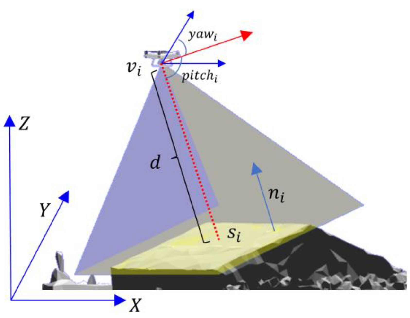
The target point is used to calculate and adjust the corresponding viewpoint position and orientation. For target point si, the corresponding viewpoint vi is generated as shown in Figure 3. The pose of the viewpoint vi can be transformed from (x, y, z, −nxi, −nyi, −nzi) into (x, y, z, yaw, pitch) by the Rodriguez formula and angle decomposition, as shown in Equation (1), which is then provided for UAV to capture images. Rod (a, b) represents the rotation matrix of vector a rotated around the a × b axis to vector b. ni = (nxi, nyi, nzi) is the normal vector of the target point si. sightbefore and ybefore are the original sight vector and the y-axis of the image coordinate system when (yaw, pitch, roll) = 0, respectively. Sightafter is the photographic sight which is −ni. Note that the equation roll ≡ 0.0 can be adopted to judge whether the angle yaw and pitch are correctly calculated.
v i = x i , y i , z i = s i + d n i R 1 = R o d s i g h t b e f o r e , s i g h t a f t e r R 2 = R o d R 1 y b e f o r e , s i g h t a f t e r × Z y a w , p i t c h , r o l l = a n g l e d e c o m p o s t i o n ( R 2 R 1 ) ,   r o l l 0.0
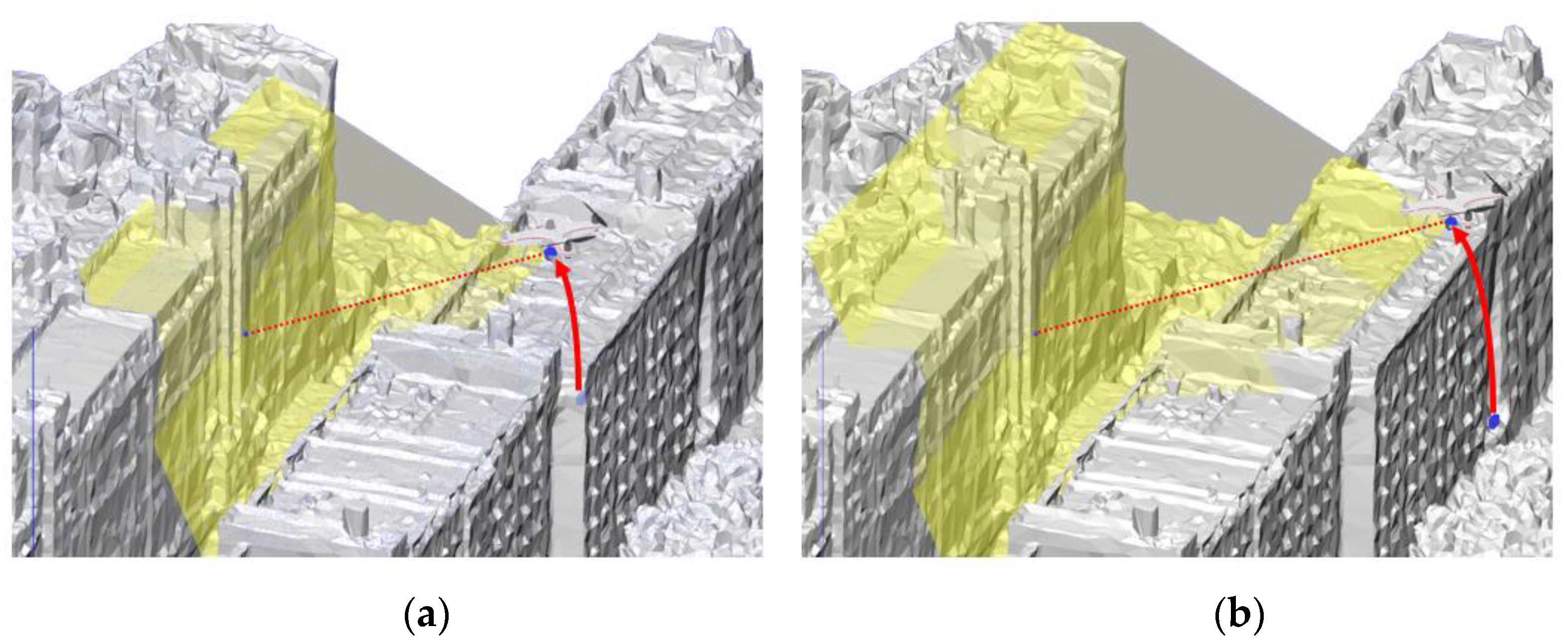
When the shooting distance is far, the generated viewpoint may be inside an obstacle, as shown in Figure 4a, and there may be obstacles between the sight of the viewpoint and the target point, as shown in Figure 4b. To avoid this situation, we fix the distance from the viewpoint to the target point, controlling the viewpoint orientation and the normal vector of the target point within a certain angle range. Then, we sample candidate viewpoints within a certain spherical range of area and search for other unobstructed viewpoints, as shown in Figure 4.
  • Reconstruction Heuristics
The sample point is used to evaluate the reconstructability of the scene by calculating its reconstructable value which indicates whether the neighbor region can be reconstructed well. Usually, a greater number of sample points would be generated on the proxy surface to better represent the reconstructability of the scene. Note that there is no viewpoint corresponding to the sample points.
A mathematical model that can evaluate the reconstructable value is needed. Some related works [4,15,16,20,22,34,42] have studied this problem, considering factors including shooting distance, observation angle, parallax angle, multi-view observation, etc. Considering the computational complexity and the theoretical integrity, the heuristics proposed by [20] are adopted, as shown in Equation (2). H(s, V) represents the reconstructable value (hereinafter referred to as H) of sample point s calculated from all viewpoints V. c s , v i , v j represents contribution of two viewpoints v i , v j to s, and v s , v i is a binary function that evaluates the visibility of sample to vi.
H s , V = i = 1 V , j = i V v s , v i v s , v j c s , v i , v j
Many researchers have studied the reconstruction mechanism. According to [4,31], the reconstruction can be satisfied when the three rays observe the same point at the same angle of 15 degrees, based on which the minimum threshold HT is calculated at about 1.30. According to [20], when H > 3, the depth error of the sample point hardly changes. According to [24], when H > 5, the Spearman correlation between the H and the accuracy of the sample point decreases sharply, floating around 0.1. Therefore, in the subsequent optimization, we keep the H of each sample point between 1.3 and 5.0 and set the minimum threshold to 1.3 to satisfy the reconstruction. If it exceeds 5.0, redundancy is considered to exist in the visible viewpoints.
For polygon primitives, we calculate its two-dimensional enveloping rectangle, then generate sample points and target points with a grid pattern according to different intervals within the rectangle, and judge whether the point falls within the polygon range. For line primitives, we directly sample equidistantly, and when the extracted edge is short, its center with normal vector is directly taken as the sample point and target point, which is the same as the operation of point primitives.

3.2.2. Optimization Objective Function

The internal normal vectors of the extracted polygon primitives are consistent. When we generate viewpoints according to certain rules, such as the overlap ratio, if the images captured at the viewpoints can realize the high-quality reconstruction of the internal polygon region, we can generate viewpoints quickly with a preset overlap ratio to realize the coverage of the polygon region. The time complexity of this step is O(n), where n is the number of target points. In most scenes, especially in urban scenes, when we segment the plane on rough proxies, polygon and line primitives can represent most surfaces and edges, respectively. In this way, we can speed up the viewpoint optimization process significantly. We construct an objective function, as shown in Equation (3), which divides viewpoint optimization into two steps.
V = a r g m i n V 1 s i S p o l y g o n + S l i n e [ H s i , V 1 H T ] + a r g m i n V 2 s j λ S u n r e c o n [ H s j , V 1 + V 2 H T ] s . t . H > H T ,   λ 85 % ,   95 %
The viewpoint set V1 for the polygon and line primitives is generated first. We consider these viewpoints an initial set for achieving the global optimum, which realizes the coverage of most parts needed for reconstruction in the urban scene, especially. Subsequent viewpoint optimization is performed to obtain V2 for point primitives, that is, fragmentary details in the scene. Spolygon represents the sample points generated in polygon primitives, and the same for lines and points. Sunrecon represents the unreconstructable sample points after adding viewpoints generated for polygon and line primitives, which is composed of Spoint and a small proportion of Spolygon and Sline. HT is set at 1.3. In addition, λ ∈ (85%,95%) is set, which means that we do not require that all fragmentary details, especially the trees, satisfy the reconstructability, which is difficult to achieve.

3.2.3. Initial Optimal Set for Polygon and Line Primitives

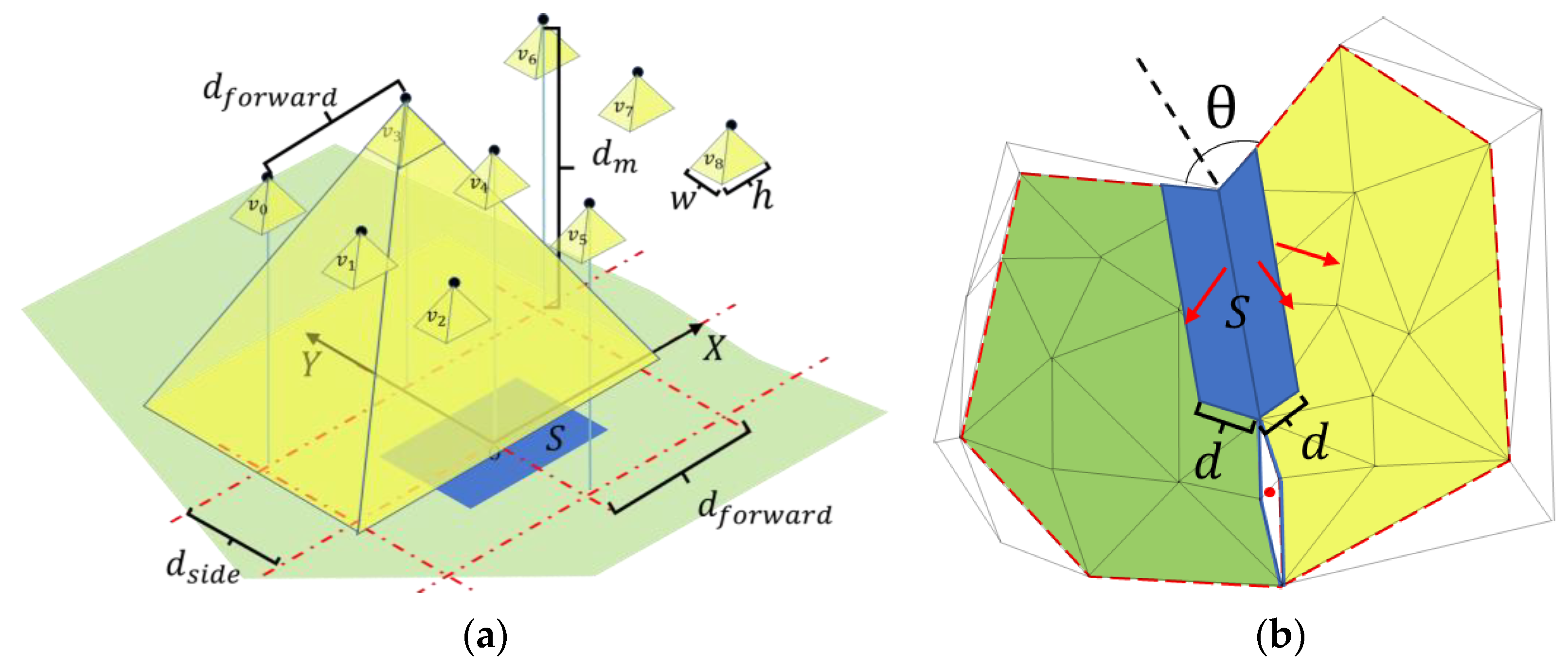
To guarantee reconstructability, we need to calculate a proper forward and side overlap based on Equation (2) to generate aligned target points and viewpoints. We construct a mathematical model for measuring the reconstructability of polygon primitives, as shown in Figure 5a, where d s i d e = 1 A h G S D ,   d f o r w a r d = 1 B w G S D ,   d m = f G S D . GSD (Ground Sample Distance) represents the length on the ground corresponding to a pixel with the unit of cm/pixel. A and B represent the side and forward overlap ratio, respectively, and f is the focal length in pixels. Furthermore, w and h are the pixels of the image in width and height. We convert the first half of the objective function into Equation (4) and calculate the optimal overlap ratio which keeps the H of each sample point in S exceeding the minimum threshold HT. S is shown as the blue area in Figure 5a which corresponds to the central range of v4, while other regions in the polygon primitives would correspond to other viewpoints. The viewpoint set V(A,B) only includes 9 viewpoints since the outer 16 viewpoints only contribute to the reconstruction of region S when the overlap exceeds 66%.
A , B = a r g m i n s i S H s i , V A , B H T ,   s . t . H > H T V A , B = v i | v x i d f o r w a r d , 0 , d f o r w a r d , v y i d s i d e , 0 , d s i d e , v z i = d m i = 1 , 2 , 9 , S = s i | s x i d f o r w a r d 2 , d f o r w a r d 2 , s y i d s i d e 2 , d s i d e 2 ,   s z i = 0
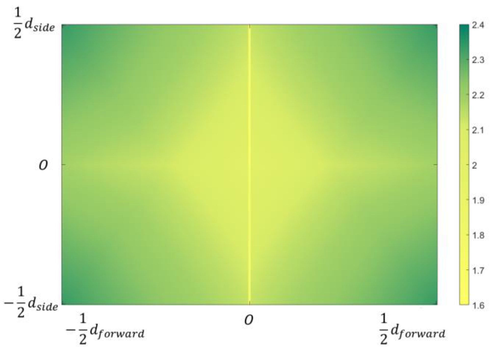
We calculate the optimal forward and side overlap with parameters of the camera mounted on commonly used DJI P4RTK, with a resolution of 4864 × 3648, a focal length of 8.8 mm and a pixel size of 2.4 microns. We set the search range from 66% to 33%. Iterative calculation finds that 50% for both forward and side overlap ratio is the optimal solution of Equation (4). The H distribution in area S is shown in Figure 6. It can be found that the distribution of H is relatively uniform, and the H of every point in S exceeds HT. When the overlap is 50%, each sample point in the blue area in Figure 5a can be uniformly covered by four images.
However, according to Figure 5a and Equation (4), the relative distribution of the viewpoint set V(A, B) and the sample point set S is related to the three factors: w, h, and f of the camera. The GSD only affects the scale of the scene model in Figure 5a. In fact, when calculating the parallax angle α between two viewpoints, it is found that for the same GSD, the FOV (Field of View) and image frame would have an impact on α, which in turn affects the H. Thus, we consider two independent variables, w/f and w/h, to further verify the effectiveness of the 50% forward and side overlap. w/f corresponds to the FOV, while w/h corresponds to the image frame which is commonly 4:3 and 3:2. We calculate the coordinates of sample points in area S and the nine viewpoints in V(A, B) with different w/f and w/h, and then obtain the average and the minimum reconstructable value of sample points in the region S, as shown in Figure 7. For commonly used UAVs and cameras like DJI P4RTK, DJI M300, and Nex7 used by [20], a 50% overlap ratio can ensure that each sample point inside the polygon primitives can be reconstructed. Moreover, from Figure 7, it can be found that the reconstructable value is maintained above 2.0 when the FOV is in the range of 30–55 degrees which is considered to be the appropriate camera FOV with an overlap ratio of 50% for acquiring images.
The mathematical model in Figure 5a only considers the interior of polygon primitives. However, there are still uncovered edge regions, as shown in the blue area in Figure 5b. The same calculation is also employed to generate target points and viewpoints on line primitives, which proves that all sample points in the blue area can be reconstructed when θ is between (75°, 270°) with a 50% overlap ratio. If the reconstructability is still not satisfied, two additional viewpoints are generated according to the normal vector of its adjacent polygons to ensure the reconstructability. Through the complementation of adjacent polygons and line primitives, all points on the edges of polygon primitives can be reconstructed.
The overlap ratio of 50% Is Ideal without considering the influence of viewpoint adjustment for obstacle avoidance. For cameras with wider FOV, the 50% overlap ratio may not guarantee that every sample point could be well reconstructed. While images from other viewpoints would compensate for the reconstructability of unreconstructable areas, we still recommend choosing an overlap ratio between 53% and 60% for polygon and line primitives to generate target points and viewpoints. The overlap range is set for three reasons: (1) when the overlap is more than 50% in both forward and side directions, each sample point can be covered by at least four images and meet the reconstructability; (2) considering the effect of camera distortion, the closer to the edge, the greater the distortion, so the overlap is set to a minimum of 53%; (3) to avoid redundancy from high overlap, the upper limit is set to 60%. However, this is an empirically derived range, and we strongly recommend no less than 53%, but the upper limit can be improved appropriately according to the complexity of the scene.
Note that a dense sampling whose density is much higher than [16,20,24,30,31,32,34] is performed in S, resulting in a more representative measurement of the reconstructability of polygon and line primitives. However, densely sampling is only performed to compute the suitable overlap ratio and verify its effectiveness. Since the internal normal vector of each primitive is consistent, each generated sample point can represent a certain area around it compared with random uniform sampling. In addition, their reconstructability has been almost satisfied by the preset overlap ratio. Hence, fewer sample points need to be generated on polygon and line primitives to judge their reconstructability. In subsequent submodular optimization, the sample points for judging reconstructability including unreconstructable sample points are directly transformed from target points generated with preset overlap ratio on polygon and line primitives, whose amount is relatively low.

3.2.4. Submodular Optimization for Point Primitives

For polygon and line primitives, we have generated an optimized initial set of viewpoints that already cover most surfaces in the scene. However, for small details in the scene, if all point primitives are performed as target points, a large number of viewpoints would be generated. It would result in redundancy, especially when the proxy tends to be more detailed, such as the proxy obtained by oblique photography. We also only need fewer images to cover the details of the scene while maintaining a high-quality reconstruction result. To better restore the details in the scene and maximize the gain from each viewpoint, we construct a submodular formulation as shown in Equation (5). The point primitives are converted to sample points and target points simultaneously to measure reconstructability and generate viewpoint set V p for optimization. Through submodular optimization, we can select one viewpoint each time with the largest information gain, so that fewer viewpoints are produced to cover the details.
v i = a r g m a x   E H ,   v i V p E H = s S v i [ exp H T H s , V 1 ] A s
Unlike [15] directly calculating the actual H gain of each viewpoint during iterations, we select the viewpoint expected to obtain the maximum gain EH calculated by Equation (5). From Equation (5), the optimal viewpoint whose sum reconstructability of its visible sample points is the smallest is selected for the current iteration. It is considered that adding this viewpoint will bring a greater expected gain. As refers to the area of the neighbor region the sample point represents, which is a weight parameter. Svi is the set of unreconstructable sample points visible from viewpoint vi. H(s,V) is the reconstructable value of s calculated from the current optimized viewpoint set V. Compared to the O m m ^ n ^   time complexity of [20,31] with the same heuristics, ours is only O( m ^ n ^ ) in each iteration, where m ^ is the average number of viewpoints visible to a sample point, n ^ is the opposite, and m is the number of viewpoint points. We can easily find that this formula satisfies the condition of submodularity, as when the H of every sample point increases, the EH decreases. After each new viewpoint is added, H is updated for the sample points seen by the viewpoint, and a new viewpoint is recalculated until the income EH is less than 0. In this way, the process of viewpoint optimization is very fast. Moreover, we can determine the required number of viewpoints to ensure details coverage without adding too many viewpoints.

3.3. Shortest Path Connection

To maximize the effectiveness of the UAV and evaluate the quality of the final generated path, we construct a mathematical model to measure energy consumption and flight time based on the UAV flight dynamics theory [43,44]. The mathematical model is shown in Equation (6). The following loose assumptions are set to simplify the complexity of the mathematical model. We consider that the air density at different heights remains the same. Statistics have found that the air density change is minimal when the height difference is within 300 m. Energy consumption only considers work against gravity and work against resistance. When overcoming the resistance, it is considered that the UAV always keeps a stable speed without acceleration and deceleration. In addition, we assume that the energy consumption of the UAV orientation change is minimal, and the most power consumption is used to keep the UAV hovering when changing the orientation. Since gravity is a conservative force, we consider that the energy consumed to overcome gravity when the drone hovers is the same as when the drone rises and then descends to the same position [44].
P d r a g = 1 2 C D A D v 3 ,   Q d r a g = P d r a g T d r a g P l i f t = W 3 2 2 D B ,   Q l i f t = P l i f t T l i f t
Tlift is the time from takeoff to landing, and Tdrag is the time for drone flight motion. CD is the wind resistance coefficient; A is the front-facing area of UAV in m2; B is the area of the rotor disc, which refers to the plane formed by the rotating rotor blades of rotorcraft. D is the air density, v is the flying speed of the drone, and W is the weight of the drone itself. To achieve high-precision positioning and attitude shooting, the drone needs to hover and adjust the orientation of the drone to control the yaw, and adjust the gimbal to control the pitch. The time that the drone hovers to change the orientation is considered. We define the relationship between hovering angle and time according to the experiments performed by [30].
According to the above model, we can realistically simulate the energy consumption and time of the UAV capturing images along the path. When we input the viewpoint sequence V = V 1 , , V i , V n   , n 2 , the time and energy consumed during a flight can be obtained. For the follow-up calculation, the parameters of commonly used M300 UAV are substituted into Equation (6) for calculation.
After obtaining the optimized set of viewpoints, we need to connect these viewpoints into a flight path and provide it to the UAV, which is a typical TSP problem. The method of [45,46] is adopted to calculate an approximately optimal path connection scheme through the ACO (Ant Colony Optimization) algorithm. Each viewpoint is a node in the graph, and we calculate the energy consumption between two viewpoints as the cost between the nodes based on Equation (6). When calculating the cost, we must determine whether the path between the two nodes passes through an obstacle, in which situation we consider the cost infinite. To speed up the subsequent path calculation process, we adopt the k-proximity method and only calculate the cost of the 20 nodes closest to each node.

4. Results

To comprehensively evaluate the effectiveness of our SGP-G method, some metrics are set to evaluate the quality of the path and the final reconstructed model. Experiments are performed both on real and virtual scenes, including the UK, Goth, and NY scenes of [20], the School, Town scenes of [47], and our Zhlp scene constructed from Urban City, as shown in Figure 8. Three types of proxy are adopted, including 2.5D box, 2.5D coarse and 3D inter. The proxy of 3D inter retains more details of the scene with more triangular faces, and 2.5D coarse retains only the range and elevation of buildings, while 2.5D box is composed of simpler bounding boxes.
The commonly used Context capture software is used to recover 3D models from images. Considering the camera distortion and the different detailed proxies, the forward and side overlap ratio of 53–60% is adopted to generate viewpoints of polygon and line primitives.

4.1. Evaluation Measures

We comprehensively evaluate the methods from two aspects: path quality and model quality. For the former, the number of viewpoints, path length, ideal flight time and energy consumption calculated based on [43,44] are evaluated. As for the model quality, the average GSD and RMS meter of the aerial triangulation process is measured, as well as the precision and recall of the reconstructed model. In addition, the visual fidelity of the reconstructed model on some details is also compared.
Especially, the metrics of precision and recall are similar to error and completeness brought up by [20]. We uniformly sample the recon (Reconstructed) and gt (Ground Truth) models at 400 pts/square meters to obtain recon points and gt points [48], so that the distributions in the two point clouds are appropriately the same. For each point in the recon points, we calculate the closest distance to gt points. Given a certain distance threshold d, we calculate the percentage of recon points whose distance is less than d. We set the distance threshold d = 0.1 m, which can better reflect the poor-quality area in the model. That is, the area where the distance with the nearest corresponding point is more than 0.1 m is considered poorly reconstructed. The percentage is then called precision (0.1). In turn, we calculate the percentage of gt points whose distance from the closest point in recon points is less than d, which is then called recall (0.1). A higher percentage means better quality of the reconstructed model. F S c o r e = 2 p r e c i s i o n 0.1 r e c a l l 0.1 p r e c i s i o n 0.1 + r e c a l l 0.1 is also calculated, which is a common measure for binary classification and suitable for the comprehensive evaluation of model quality. In addition, we count the distances at which 90% of the points in the recon and gt models are smaller, and precision(90%) and recall (90%) are obtained, respectively.

4.2. Self-Evaluation

4.2.1. Impact of Different Detailed Proxy

Three virtual scenes, including UK, Town and School, are used to measure the difference of plane segmentation in different detailed proxies. Among them, UK mainly includes relatively regular buildings; Town includes irregular buildings, bridges and trees; School includes suspended buildings with repeated texture of ground areas. Plane segmentation is performed on proxies containing varying levels of detail, and then geometric primitives are extracted, as shown in Figure 9.
For regular and simple proxies, such as 2.5D box and 2.5D coarse, the segmentation is neat because only the range and elevation information are retained with fewer details. There are more details in the proxy of 3D inter, leading to messier segmentation results. However, regardless of the type of proxy used, the extracted primitives can reflect the geometric composition of the proxy well.
The impact of different detailed proxies on the reconstruction results is also evaluated on Town and School scenes. Both scenes contain some details that the 2.5D model cannot represent. We generate a photographic path with a GSD of 0.7 cm/pixel based on the extracted primitives, and then reconstruct the model. The calculated precision and recall of the reconstructed model are shown in Table 1.
It is straightforward to see that precision and recall are on the rise in general for proxy from rough to fine, which aligns with our expectations, especially on School scene. The precision drops with more images on School from 2.5D coarse to 3D inter. It is considered normal, as when the reconstructability of the scene is already guaranteed by sufficient coverage, adding additional images may lead to decreased precision [30].
The overall model quality is satisfying, proving that our method is relatively robust for proxies with different detailed proxies. Although the precision is low for the 2.5D box proxy of School, the recall is not. Moreover, a higher overlap ratio, such as 60%, can make up for the impact of the proxy being too simple. Experiments show that when we adopt an overlap ratio of 60% for the 2.5D box proxy to generate 263 images, the precision and recall are improved to 85.60% and 49.30%, respectively.

4.2.2. Impact of Overlap Ratio

We have theoretically verified the rationality of the 50% forward and side overlap ratio by calculating H in Section 3.2.3. In addition, we generate viewpoints from polygon and line primitives by combining multiple overlap ratios to verify rationality by calculating precision and recall. To avoid the influence of point primitives generated by the details, the experiment is performed on Zhlp scene. Zhlp includes three regular buildings with a few non-planar details, which can better reflect the effect of the overlap ratio on reconstruction. We generate viewpoints with forward and side overlap ratios of 45–45%, 53–53%, 60–60%, and 66–66%, respectively. In particular, specific overlap ratios of 66–33% and 66–8% are adopted, which also ensure that at least three viewpoints cover the sample points.
The quantitative evaluation of the reconstructed model is shown in Table 2. Reconstructable percent represents the proportion of the uniform sample points [48] that satisfy the reconstructability according to its H and the threshold HT. From Table 2, the aerial triangulation is prone to failure when the reconstructable percent is relatively low, such as ratios of 45–45% and 66–8%. Higher overlap rates do not significantly improve recall and accuracy when the overlap rate is greater than 53%. For the 66–33% overlap ratio, the precision and recall decrease and the number of images increases. It is clear that our preset overlap ratio range is reasonable, and a 53% overlap ratio can achieve good results with fewer viewpoints. Increasing the overlap ratio can also lead to some improvement in precision and recall if the limitation on the number of images is not considered.

4.2.3. Effectiveness of Submodular Formulation

Submodular optimization is performed on viewpoints from point primitives to cover fragmented details with little redundancy. To verify the effectiveness of the submodular optimization strategy, the 3D inter proxies of School and Town are adopted to generate optimal viewpoint sets Φ, Φ + 15, Φ + 30, Φ + 50, and viewpoint set when the automatic iteration terminates, respectively. Φ is the viewpoint set generated from polygon and line primitives. A 2.5D proxy is not suggested, as it would generate fewer point primitives. We calculate the estimated gain EH by Equation (5) and ΔH which is the actual H gain of unreconstructable sample points for each iteration after adding the viewpoint with maximum EH, as shown in Figure 10. Based on images captured from viewpoints, we reconstruct the 3D model and calculate the recall, as shown in Table 3.
From Figure 10 and Table 3, the EH calculated by the submodular function can almost represent the actual H gain. Their trends are consistent, which verifies that submodular optimization is reasonable. Furthermore, when the set contains viewpoints generated for polygon and line primitives, the recall has already reached a high level. As the number of viewpoints increases, the recall increases slowly, reflecting the diminishing marginal effect of submodular optimization. When the convergence condition we set is reached, the recall hardly increases, which shows that our convergence conditions are reasonable. In addition, we find that the reconstructability can already be generally satisfied by only the viewpoint set generated for polygon and line primitives, which proves that it is a suitable initial value to approximate the global optimum.

4.3. Comparison to State of the Art

  • Comparison with [20]
To verify the effectiveness of our SGP-G method, we compare it with [20] on NY, Goth and UK. Since its gt model cannot be obtained, three metrics based on its evaluation tool are evaluated, including Precision, Local Completeness (hereinafter referred to as LComp) and Global Completeness (hereinafter referred to as GComp). The evaluation from these three metrics is completed similarly to precision and recall. The difference is that the distance threshold is set as 0.05 m and 0.075 m for LComp. For GComp, we modified the parameters and set the distance threshold to 0.5 m and 0.75 m to measure the percentage of the unreconstructed part. For a fair comparison, the same camera with pixel size of 3.9 microns, resolution of 6000 × 4000 and focal length of 14.16 mm are adopted to generate the flight path and capture virtual images. In addition, we set the GSD of the captured image to be consistent with its average GSD. Table 4 shows the comparison with [20] on UK, Goth and NY with a 2.5D coarse proxy.
On all three scenes, our precision is close to the [20]. For LComp, it is ahead of us except for the UK scene. Considering the large number of images it generates, it is reasonable that it achieves better quality on some details. We obtain slightly better results on UK scene which is relatively regular. For GComp, our completeness is slightly higher on all three scenes, indicating that our method is close to [20] in model quality and even slightly better. Note that under the same GSD, its images are nearly two times ours, resulting in a long-time reconstruction process. Furthermore, because the viewpoints from polygon primitives are regularly arranged, our path length, time and energy consumption are smaller, even less than half by comparison. Compared with [20], we consume less time during path generation, UAV flight and reconstruction with comparable model quality.
  • Comparison with [30,31]
Additionally, School and Town in Urban Scene3D are adopted to compare with the methods of [30,31], respectively. For a fair comparison, we use the same camera with a pixel size of 3.9 microns, resolution of 6000 × 4000 and focal length of 20.30 mm, and we keep the average GSD consistent with them when generating the path. We choose two overlap ratios of 53% and 60%. In the aerial triangulation stage, the capturing positions of the images are all imported.
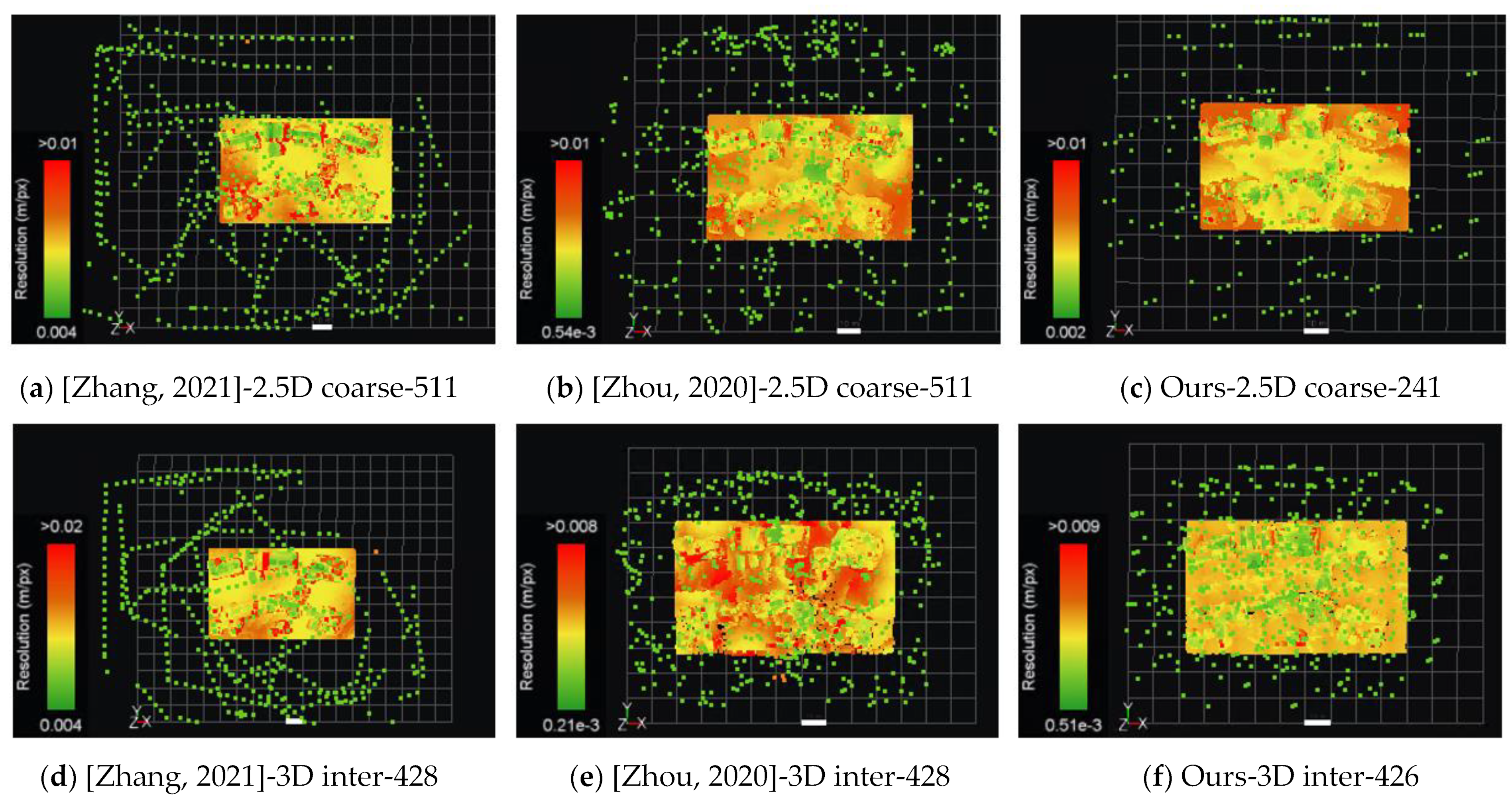
Figure 11 shows the viewpoint distribution and reconstructed scene resolution generated on Town scene with two proxies. It is directly visualized by Context Capture after the aerial triangulation, where color represents the size of one pixel on the ground, that is, the GSD. For the viewpoint distribution, that of [30] as well as its path are very regular, but the shooting distance is significantly farther. Therefore, with a 3D inter proxy, the same number of images results in a much lower resolution than [31] and ours. Our image distribution is more regular than that of [31], as polygon and line primitives are utilized to generate regular viewpoint arrays, especially with a 2.5D coarse proxy. As for the resolution, ours is significantly more uniform than the other two methods and maintains an excellent level, especially with 3D inter proxy, as shown in Figure 11f. Our resolution value looks higher with a 2.5D coarse proxy, as shown in Figure 11a–c. However, switching the perspective, as shown in Figure 12, our resolution is still close to [31] or even better. In addition, the number of our images is much smaller than that of [30,31].
Table 5 and Table 6 show the comparison between ours and [30,31] on School and Town scenes. The designation Ours-53%-0.7 refers to generating a path with an overlap ratio of 53% and a distance corresponding to a GSD of 0.7 cm. For the coarse proxy, the difference between the designed GSD and the average GSD calculated by aerial triangulation is relatively large due to its simplicity, as shown in rows (3, 9) of Table 5 and Table 6. However, the difference in GSD is tiny for the inter proxy, as shown in rows (6, 12) of Table 5 and Table 6, indicating that the path we designed can reach the expected resolution with a detailed proxy.
From Table 5, regardless of scene and proxy, the precision and recall of [30] are significantly behind ours with even more images. Due to its flight height, the average GSD is significantly larger, resulting in low resolution of the building side, as shown in Figure 11 and Figure 12. Moreover, the length of its path is not ahead and even consumes more time and energy with a further shooting distance, even if a continuous path is connected.
From Table 6, compared with [31], the RMSE of our reprojection is the lowest in both scenes, keeping close cases in terms of precision and recall. Overall, except for the 2.5D coarse proxy on School scene, our method is slightly ahead in the F-score. Figure 13 visually shows the comparison between the details of the reconstructed model with [31]. Compared to it, we obtain better visual fidelity of these details, since we generate sample points for building corners and fragmented details in a more targeted manner.
Overall, considering the evaluation of path quality and model quality, we obtain a higher quality with less energy consumption and fewer images, which illustrates that our method reaches the state of the art.

4.4. Field Test

Experiments on three real scenes are also conducted. The viewpoints generated from different primitives and unreconstructable sample points during the optimization process are shown in Figure 14. Regularly arranged viewpoints generated from polygon and line primitives, which can basically realize the reconstructability of flat areas, are obviously seen in Figure 14a,b. With only viewpoints generated from polygon and line primitives, the unreconstructable sample points mainly concentrate in fragmented areas. After the whole optimization, there are only a few sample points that cannot satisfy the reconstructability, which are mainly located in narrow and slender areas.
We compare our method with the regular baseline pattern in oblique photogrammetry on the Museum scene, which flies at a fixed altitude with a five-direction camera over the scene to capture the images. The DJI P4RTK is adopted to capture images, which is a UAV intended for the mapping field mounted with a camera with a pixel size of 2.4 microns, resolution of 5472 × 3648 and focal length of 8.8 mm. To keep nearly the same number of images, the desired GSD for the oblique photography and ours is set as 1.2 cm and 0.6 cm, respectively. The point clouds captured from 21 sites by FARO FOECUS S350 are adopted as ground truth to evaluate the precision and recall. Figure 15 shows the visual fidelity comparison of some details. Table 7 lists the quantitative comparison in the final reconstructed quality. We can see that our method is far ahead of oblique photography in precision and recall. It is mainly because we adopt a close photographic way that can adjust the orientation to obtain more information about the details in the scene.

5. Discussion

Compared with other methods, the most prominent feature of our method is the efficient utilization of geometric primitives extracted from the proxy, based on which the viewpoint optimization for the reconstruction of the whole scene is transferred into the reconstructable optimization problem of each primitive. Moreover, the geometric primitive has various positive effects on subsequent steps.
First, a more representative evaluation of reconstructability is realized by primitives. Every triangle on the proxy surface is segmented into a special primitive, and its reconstructability is measured. Compared with uniform sampling of [16,20,24,30,31,32,34] which easily ignores fragmented details and edges, we fully consider the coverage of large areas in the scene based on polygon primitives, and then consider the reconstructability of every fragmented detail in the scene based on line and point primitives.
Second, two viewpoint optimization strategies are performed on different primitives, which greatly accelerates the optimization process, as shown in Table 4. An initial set of viewpoints that can almost satisfy the reconstructability of polygon and line primitive is generated directly at a preset overlap ratio, which is considered as an initial value for global optimum with no further optimization, as shown in Table 3 and Figure 14b. For point primitives, we establish a submodular formula to augment a few viewpoints to improve the reconstruction of details and minimize redundancy. The optimization is only performed on the viewpoints generated by the point primitives. Changing the GSD of the desired model and images does not affect the number of viewpoints for point primitives, thus the computation time consumed is generally unchanged. Compared with the methods of [20,30,31,34], our SGP-G method realizes a near-global optimum with almost no optimization.
Finally, for flat areas in the scene, such as building facades and ground, regularly arranged viewpoints with the same orientation are generated from polygons and line primitives, as shown in Figure 11c and Figure 14a. Compared with [20,31], our viewpoints prefer a more regular arrangement and smoother angle change of the final connected path, resulting in less consumption of time and energy, as shown in Table 4 and Table 5.
In all, our method achieves viewpoint selection and optimization in a relatively simple way and exhibits extraordinary performance in all aspects. There are also some limitations to our method. First, the mesh segmentation method is limited in many situations. We currently use the bottom-up method of plane segmentation to extract primitives, which requires correct triangular information of proxy. In future work, we hope to use a top-down segmentation method and iteratively split the bounding box to obtain a more regular representation of the proxy, which is similar to the LOD2 model in GIS. Second, cross-direction and multi-resolution combined photography is not considered. Although the workload of optimization computation increases when considering them, there is lower information entropy in the image of the cross-direction shooting, which can better capture the side information of the scene. Furthermore, low-resolution images are also more suitable for reconstructing weak texture areas. We hope to conduct in-depth research on how to capture images with multi-resolution and multi-orientation to reconstruct higher-quality models in future work.

6. Conclusions

In this article, we propose a surface geometric primitive-guided UAV path planning method (SGP-G) for high-quality image-based 3D reconstruction. There are significant improvements in three aspects of our method based on the extracted primitives. First, the generated primitives with consistent normal vector assist in comprehensively assessing the reconstructability of the whole scene. Second, an initial viewpoint set which is considered a better initial set for global optimum is generated to satisfy the reconstructability of most areas with an appropriate overlap ratio, which greatly speeds up the optimization process. Third, a well-aligned path is generated with smaller turns and less time and energy consumption. The experiments show that our method is applicable to different detailed proxies. Compared with the state of the art, we can plan photography paths with higher efficiency, and finally achieve 3D reconstruction with equal or higher quality with fewer images. Our method provides a fast UAV 3D path planning method for image-based 3D reconstruction, which is useful for the acquisition of high-quality models in engineering.

Author Contributions

Conceptualization, Z.J. and H.Z.; methodology, H.Z.; software, Z.J., H.Z., S.L. and K.Z.; validation, H.Z. and X.Y.; formal analysis, H.Z.; investigation, H.Z. and Y.L.; resources, H.Z., K.Z. and X.Y.; data curation, H.Z. and X.Y.; writing—original draft preparation, H.Z., Y.L. and X.Y.; writing—review and editing, H.Z. and Y.L.; visualization, Z.J., H.Z. and L.C.; supervision, Z.J.; project administration, Z.J. and X.H.; funding acquisition, Z.J. and X.H. All authors have read and agreed to the published version of the manuscript.

Funding

This research was funded by Anhui Province Natural Science Foundation, grant number 2208085QD106.

Data Availability Statement

Some of the datasets used in this study are openly available. These datasets can be found at https://vccimaging.org/Publications/Smith2018UAVPathPlanning/ (accessed on 18 December 2021) and https://vcc.tech/UrbanScene3D (accessed on 21 July 2022).

Acknowledgments

The authors would like to thank the anonymous reviewers for their constructive comments.

Conflicts of Interest

The authors declare no conflict of interest.

References

  1. Aharchi, M.; Ait Kbir, M. A Review on 3D Reconstruction Techniques from 2D Images. In Innovations in Smart Cities Applications, 3rd ed.; Ben Ahmed, M., Boudhir, A.A., Santos, D., El Aroussi, M., Karas, İ.R., Eds.; Springer International Publishing: Cham, Switzerland, 2020; pp. 510–522. [Google Scholar]
  2. Ma, Z.; Liu, S. A Review of 3D Reconstruction Techniques in Civil Engineering and Their Applications. Adv. Eng. Inform. 2018, 37, 163–174. [Google Scholar] [CrossRef]
  3. De Reu, J.; De Smedt, P.; Herremans, D.; Van Meirvenne, M.; Laloo, P.; De Clercq, W. On Introducing an Image-Based 3D Reconstruction Method in Archaeological Excavation Practice. J. Archaeol. Sci. 2014, 41, 251–262. [Google Scholar] [CrossRef]
  4. Furukawa, Y.; Hernández, C. Multi-View Stereo: A Tutorial. Found. Trends® Comput. Graph. Vis. 2015, 9, 1–148. [Google Scholar] [CrossRef]
  5. Westoby, M.J.; Brasington, J.; Glasser, N.F.; Hambrey, M.J.; Reynolds, J.M. ‘Structure-from-Motion’ Photogrammetry: A Low-Cost, Effective Tool for Geoscience Applications. Geomorphology 2012, 179, 300–314. [Google Scholar] [CrossRef]
  6. Schönberger, J.L.; Zheng, E.; Frahm, J.-M.; Pollefeys, M. Pixelwise View Selection for Unstructured Multi-View Stereo. In Proceedings of the Computer Vision—ECCV 2016, Amsterdam, The Netherlands, 11–14 October 2016; Leibe, B., Matas, J., Sebe, N., Welling, M., Eds.; Springer International Publishing: Cham, Switzerland, 2016; pp. 501–518. [Google Scholar]
  7. Seitz, S.M.; Curless, B.; Diebel, J.; Scharstein, D.; Szeliski, R. A Comparison and Evaluation of Multi-View Stereo Reconstruction Algorithms. In Proceedings of the 2006 IEEE Computer Society Conference on Computer Vision and Pattern Recognition (CVPR’06), New York, NY, USA, 17–22 June 2006; Volume 1, pp. 519–528. [Google Scholar]
  8. Snavely, N.; Seitz, S.M.; Szeliski, R. Photo Tourism: Exploring Photo Collections in 3D. ACM Trans. Graph. 2006, 25, 835–846. [Google Scholar] [CrossRef]
  9. Yao, Y.; Luo, Z.; Li, S.; Fang, T.; Quan, L. MVSNet: Depth Inference for Unstructured Multi-View Stereo. In Proceedings of the Computer Vision—ECCV 2018, Munich, Germany, 8–14 September 2018; Ferrari, V., Hebert, M., Sminchisescu, C., Weiss, Y., Eds.; Springer International Publishing: Cham, Switzerland, 2018; pp. 785–801. [Google Scholar]
  10. Yao, Y.; Luo, Z.; Li, S.; Shen, T.; Fang, T.; Quan, L. Recurrent MVSNet for High-Resolution Multi-View Stereo Depth Inference. In Proceedings of the IEEE/CVF Conference on Computer Vision and Pattern Recognition, Long Beach, CA, USA, 16–17 June 2019; pp. 5525–5534. [Google Scholar]
  11. Goesele, M.; Snavely, N.; Curless, B.; Hoppe, H.; Seitz, S.M. Multi-View Stereo for Community Photo Collections. In Proceedings of the 2007 IEEE 11th International Conference on Computer Vision, Rio De Janeiro, Brazil, 14–21 October 2007; pp. 1–8. [Google Scholar]
  12. Hornung, A.; Zeng, B.; Kobbelt, L. Image Selection for Improved Multi-View Stereo. In Proceedings of the 2008 IEEE Conference on Computer Vision and Pattern Recognition, Anchorage, Alaska, 23–28 June 2008; pp. 1–8. [Google Scholar]
  13. Fathi, H.; Dai, F.; Lourakis, M. Automated As-Built 3D Reconstruction of Civil Infrastructure Using Computer Vision: Achievements, Opportunities, and Challenges. Adv. Eng. Inform. 2015, 29, 149–161. [Google Scholar] [CrossRef]
  14. Liu, X.; Ji, Z.; Zhou, H.; Zhang, Z.; Tao, P.; Xi, K.; Chen, L.; Junior, J. An object-oriented uav 3d path planning method applied in cultural heritage documentation. ISPRS Ann. Photogramm. Remote Sens. Spat. Inf. Sci. 2022, V-1–2022, 33–40. [Google Scholar] [CrossRef]
  15. Hepp, B.; Nießner, M.; Hilliges, O. Plan3D: Viewpoint and Trajectory Optimization for Aerial Multi-View Stereo Reconstruction. ACM Trans. Graph. 2019, 38, 1–17. [Google Scholar] [CrossRef]
  16. Roberts, M.; Shah, S.; Dey, D.; Truong, A.; Sinha, S.; Kapoor, A.; Hanrahan, P.; Joshi, N. Submodular Trajectory Optimization for Aerial 3D Scanning. In Proceedings of the 2017 IEEE International Conference on Computer Vision (ICCV), Venice, Italy, 22–29 October 2017; pp. 5334–5343. [Google Scholar]
  17. Koch, T.; Körner, M.; Fraundorfer, F. Automatic and Semantically-Aware 3D UAV Flight Planning for Image-Based 3D Reconstruction. Remote Sens. 2019, 11, 1550. [Google Scholar] [CrossRef]
  18. Li, T.; Hailes, S.; Julier, S.; Liu, M. UAV-Based SLAM and 3D Reconstruction System. In Proceedings of the 2017 IEEE International Conference on Robotics and Biomimetics (ROBIO), Macau, China, 5–8 December 2017; pp. 2496–2501. [Google Scholar]
  19. Nex, F.; Remondino, F. UAV for 3D Mapping Applications: A Review. Appl. Geomat. 2014, 6, 1–15. [Google Scholar] [CrossRef]
  20. Smith, N.; Moehrle, N.; Goesele, M.; Heidrich, W. Aerial Path Planning for Urban Scene Reconstruction: A Continuous Optimization Method and Benchmark. ACM Trans. Graph. 2018, 37, 1–15. [Google Scholar] [CrossRef]
  21. Maboudi, M.; Homaei, M.; Song, S.; Malihi, S.; Saadatseresht, M.; Gerke, M. A Review on Viewpoints and Path-Planning for UAV-Based 3D Reconstruction. arXiv 2022, arXiv:2205.03716. [Google Scholar] [CrossRef]
  22. Hepp, B.; Dey, D.; Sinha, S.N.; Kapoor, A.; Joshi, N.; Hilliges, O. Learn-to-Score: Efficient 3D Scene Exploration by Predicting View Utility. In Proceedings of the Computer Vision—ECCV 2018, Munich, Germany, 8–14 September 2018; Ferrari, V., Hebert, M., Sminchisescu, C., Weiss, Y., Eds.; Springer International Publishing: Cham, Switzerland, 2018; pp. 455–472. [Google Scholar]
  23. Kuang, Q.; Wu, J.; Pan, J.; Zhou, B. Real-Time UAV Path Planning for Autonomous Urban Scene Reconstruction. In Proceedings of the 2020 IEEE International Conference on Robotics and Automation (ICRA), Paris, France, 31 May–31 August 2020; pp. 1156–1162. [Google Scholar]
  24. Liu, Y.; Cui, R.; Xie, K.; Gong, M.; Huang, H. Aerial Path Planning for Online Real-Time Exploration and Offline High-Quality Reconstruction of Large-Scale Urban Scenes. ACM Trans. Graph. 2021, 40, 1–16. [Google Scholar] [CrossRef]
  25. Palazzolo, E.; Stachniss, C. Effective Exploration for MAVs Based on the Expected Information Gain. Drones 2018, 2, 9. [Google Scholar] [CrossRef]
  26. Wu, S.; Sun, W.; Long, P.; Huang, H.; Cohen-Or, D.; Gong, M.; Deussen, O.; Chen, B. Quality-Driven Poisson-Guided Autoscanning. ACM Trans. Graph. 2014, 33, 203:1–203:12. [Google Scholar] [CrossRef]
  27. Xu, K.; Shi, Y.; Zheng, L.; Zhang, J.; Liu, M.; Huang, H.; Su, H.; Cohen-Or, D.; Chen, B. 3D Attention-Driven Depth Acquisition for Object Identification. ACM Trans. Graph. 2016, 35, 238:1–238:14. [Google Scholar] [CrossRef]
  28. Song, S.; Kim, D.; Jo, S. Online Coverage and Inspection Planning for 3D Modeling. Auton. Robot. 2020, 44, 1431–1450. [Google Scholar] [CrossRef]
  29. Schmid, L.; Pantic, M.; Khanna, R.; Ott, L.; Siegwart, R.; Nieto, J. An Efficient Sampling-Based Method for Online Informative Path Planning in Unknown Environments. IEEE Robot. Autom. Lett. 2020, 5, 1500–1507. [Google Scholar] [CrossRef]
  30. Zhang, H.; Yao, Y.; Xie, K.; Fu, C.-W.; Zhang, H.; Huang, H. Continuous Aerial Path Planning for 3D Urban Scene Reconstruction. ACM Trans. Graph. 2021, 40, 1–15. [Google Scholar] [CrossRef]
  31. Zhou, X.; Xie, K.; Huang, K.; Liu, Y.; Zhou, Y.; Gong, M.; Huang, H. Offsite Aerial Path Planning for Efficient Urban Scene Reconstruction. ACM Trans. Graph. 2020, 39, 1–16. [Google Scholar] [CrossRef]
  32. Yan, F.; Xia, E.; Li, Z.; Zhou, Z. Sampling-Based Path Planning for High-Quality Aerial 3D Reconstruction of Urban Scenes. Remote Sens. 2021, 13, 989. [Google Scholar] [CrossRef]
  33. Zheng, X.; Wang, F.; Li, Z. A Multi-UAV Cooperative Route Planning Methodology for 3D Fine-Resolution Building Model Reconstruction. ISPRS J. Photogramm. Remote Sens. 2018, 146, 483–494. [Google Scholar] [CrossRef]
  34. Liu, Y.; Lin, L.; Hu, Y.; Xie, K.; Fu, C.-W.; Zhang, H.; Huang, H. Learning Reconstructability for Drone Aerial Path Planning. ACM Trans. Graph. 2022, 41, 1–17. [Google Scholar] [CrossRef]
  35. Li, Q.; Huang, H.; Yu, W.; Jiang, S. Optimized Views Photogrammetry: Precision Analysis and a Large-Scale Case Study in Qingdao. IEEE J. Sel. Top. Appl. Earth Obs. Remote Sens. 2023, 16, 1144–1159. [Google Scholar] [CrossRef]
  36. Hoppe, C.; Wendel, A.; Zollmann, S.; Pirker, K.; Irschara, A.; Bischof, H.; Kluckner, S. Photogrammetric Camera Network Design for Micro Aerial Vehicles. In Proceedings of the Computer Vision Winter Workshop, Waikoloa, HI, USA, 3–7 January 2012; pp. 1–3. [Google Scholar]
  37. Bouzas, V.; Ledoux, H.; Nan, L. Structure-Aware Building Mesh Polygonization. ISPRS J. Photogramm. Remote Sens. 2020, 167, 432–442. [Google Scholar] [CrossRef]
  38. Castagno, J.; Atkins, E. Polylidar—Polygons From Triangular Meshes. IEEE Robot. Autom. Lett. 2020, 5, 4634–4641. [Google Scholar] [CrossRef]
  39. Castagno, J.; Atkins, E. Polylidar3D-Fast Polygon Extraction from 3D Data. Sensors 2020, 20, 4819. [Google Scholar] [CrossRef]
  40. Douglas, D.H.; Peucker, T.K. Algorithms for the Reduction of the Number of Points Required to Represent a Digitized Line or Its Caricature. Cartographica 1973, 10, 112–122. [Google Scholar] [CrossRef]
  41. Hershberger, J.; Snoeyink, J. Speeding Up the Douglas-Peucker Line-Simplification Algorithm. In Proceedings of the 5th International Symposium on Spatial Data Handling, Charleston, SC, USA, 3–7 August 1992; pp. 134–143. [Google Scholar]
  42. Peng, C.; Isler, V. Adaptive View Planning for Aerial 3D Reconstruction. In Proceedings of the 2019 International Conference on Robotics and Automation (ICRA), Montreal, QC, Canada, 20–24 May 2019; pp. 2981–2987. [Google Scholar]
  43. Abeywickrama, H.V.; Jayawickrama, B.A.; He, Y.; Dutkiewicz, E. Comprehensive Energy Consumption Model for Unmanned Aerial Vehicles, Based on Empirical Studies of Battery Performance. IEEE Access 2018, 6, 58383–58394. [Google Scholar] [CrossRef]
  44. Thibbotuwawa, A.; Nielsen, P.; Zbigniew, B.; Bocewicz, G. Energy Consumption in Unmanned Aerial Vehicles: A Review of Energy Consumption Models and Their Relation to the UAV Routing. In Information Systems Architecture and Technology, Proceedings of the 39th International Conference on Information Systems Architecture and Technology—ISAT 2018, Nysa, Polska, 16–18 September 2018; Springer: Cham, Switzerland, 2019; pp. 173–184. [Google Scholar]
  45. Dorigo, M.; Gambardella, L.M. Ant Colony System: A Cooperative Learning Approach to the Traveling Salesman Problem. IEEE Trans. Evol. Comput. 1997, 1, 53–66. [Google Scholar] [CrossRef]
  46. Skinderowicz, R. The GPU-Based Parallel Ant Colony System. J. Parallel Distrib. Comput. 2016, 98, 48–60. [Google Scholar] [CrossRef]
  47. Lin, L.; Liu, Y.; Hu, Y.; Yan, X.; Xie, K.; Huang, H. Capturing, Reconstructing, and Simulating: The UrbanScene3D Dataset. In Proceedings of the Computer Vision—ECCV 2022, Tel Aviv, Israel, 23–27 October 2022; Avidan, S., Brostow, G., Cissé, M., Farinella, G.M., Hassner, T., Eds.; Springer Nature Switzerland: Cham, Switzerland, 2022; pp. 93–109. [Google Scholar]
  48. Vose, M.D. A Linear Algorithm for Generating Random Numbers with a given Distribution. IEEE Trans. Softw. Eng. 1991, 17, 972–975. [Google Scholar] [CrossRef]
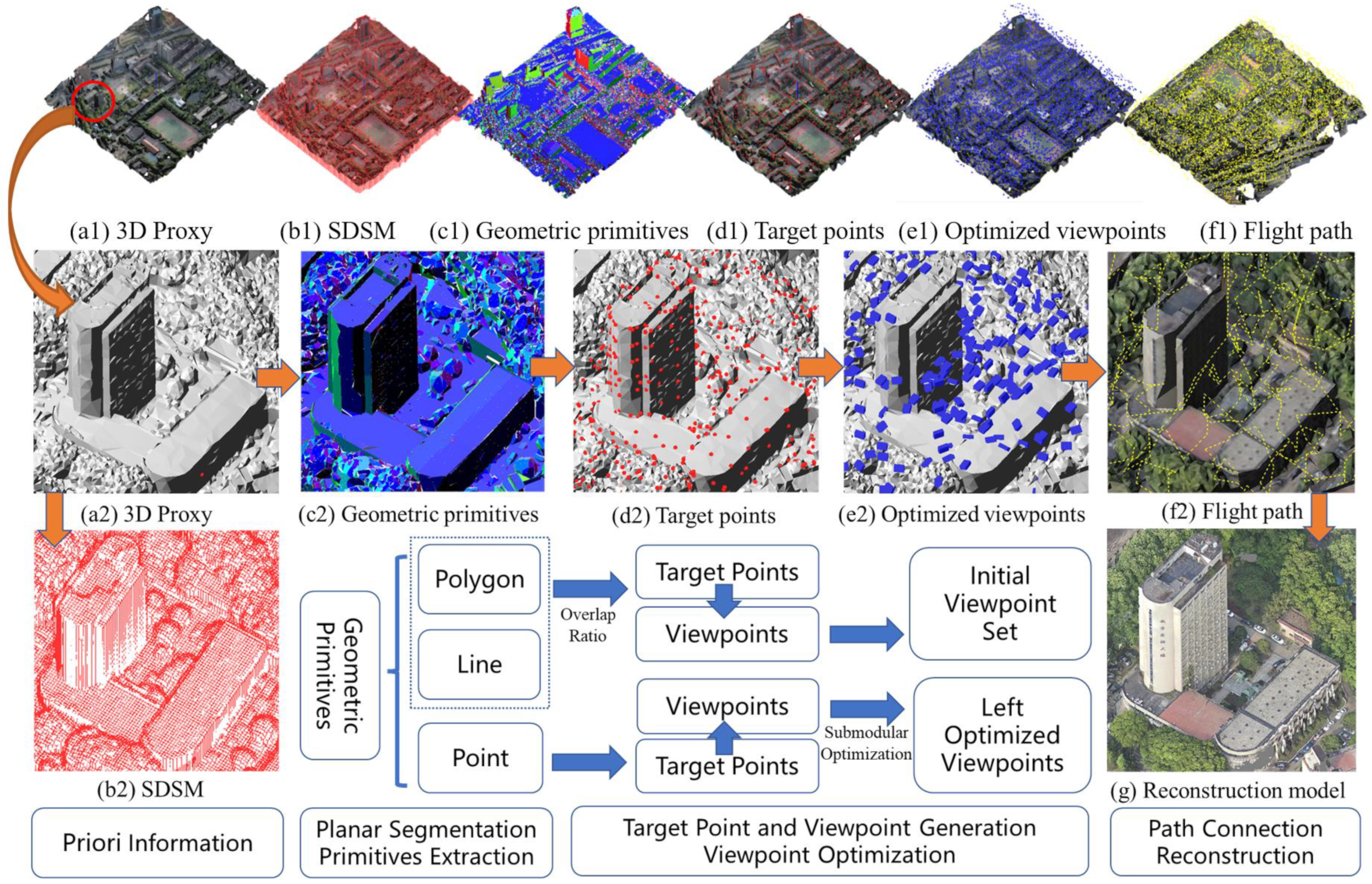
Figure 1. Flowchart of primitive-guided UAV path planning method (SGP-G). Based on the proxy (a1,a2) of campus (225,000 m2, top row) and laboratory (6400 m2, bottom row), SDSM (b1,b2) for obstacle avoidance is generated. After plane segmentation, polygon, line, and point primitives (c1,c2) are obtained. Different optimization strategies are carried out to generate the target points (d1,d2) and optimized viewpoint set (e1,e2) that meets the reconstructability. Considering energy- and time consumption, an approximate optimal path (f1,f2) connecting viewpoints is generated. Finally, the acquired image is used to reconstruct the model (g).
Remotesensing 15 02632 g001
Figure 2. The process of primitives extraction. According to the triangulation information (a), the proxy is segmented to obtain the planar regions to which each triangular surface belongs (b); the polygon, line, and point primitives (c) are then automatically extracted.
Remotesensing 15 02632 g002
Figure 3. Correspondence between the target point and viewpoint.
Remotesensing 15 02632 g003
Figure 4. Viewpoint adjustment method. Adjustment for viewpoint in the obstacle (a) and adjustment for occlusion of sight (b).
Remotesensing 15 02632 g004
Figure 5. Mathematical model for measuring the reconstructability of polygon primitives (a) and line primitives (b).
Remotesensing 15 02632 g005
Figure 6. The distribution of H calculated with camera parameters of DJI P4RTK and an overlap ratio of 50%.
Remotesensing 15 02632 g006
Figure 7. Reconstructability of different w/f and w/h with the overlap ratio of 50%.
Remotesensing 15 02632 g007
Figure 8. Different virtual scenes.
Remotesensing 15 02632 g008
Figure 9. Polygon primitives are rendered according to n x , n y , n z × 255 ; line primitives are displayed with white lines (some areas in the figure are displayed with an extra part due to the defect of drawing concave polygons directly with OpenGL, such as UK 2.5D coarse).
Remotesensing 15 02632 g009
Figure 10. Trends in the EH and ΔH when adding a new viewpoint on School (a) and Town (b) scenes.
Remotesensing 15 02632 g010
Figure 11. The resolution of Town scene (top view) with proxies of 2.5D coarse (top row) and 3D inter (bottom row) [30,31].
Remotesensing 15 02632 g011
Figure 12. The resolution of Town scene (side view) with a 2.5D coarse proxy [30,31].
Remotesensing 15 02632 g012
Figure 13. Visual fidelity comparison with [31] on School and Town.
Remotesensing 15 02632 g013
Figure 14. Viewpoints (a,c) generated from different primitives and unreconstructable sample points (b,d) during the optimization process on Mall (top row, 8535 m2), Museum (middle row, 9521 m2) and Campus (bottom row, 80,200 m2) scenes. With only viewpoints generated from polygon and line primitives (a), the unreconstructable sample points are rendered with green dots (b), which mainly concentrate in fragmented areas. Then, viewpoints for point primitives are generated and optimized (c). The final unreconstructable sample points are rendered in (d). The blue dots with white dashed lines and red dots represent the position, orientation and corresponding target point of viewpoints, respectively.
Remotesensing 15 02632 g014
Figure 15. Based on the generated path and viewpoints (a) from oblique photography (top row) and ours (bottom row), the models are reconstructed (b), and some details (c) in the models are compared.
Remotesensing 15 02632 g015
Table 1. Comparison of model quality between using different proxies. The arrows represent the trend of the values with better results on the indicators, and the following tables are the same.
SceneProxy#ImgsPrecisionRecall
0.1 m
↑%
90%
↓m
0.1 m
↑%
90%
↓m
Town
0.7 cm
53%
2.5D Box18391.470.06670.510.806
2.5D Coarse22093.040.05671.070.778
3D Inter24294.000.05371.310.769
School
0.7 cm
53%
2.5D Box19867.8330.10344.272.308
2.5D Coarse22085.790.21246.472.041
3D Inter37985.630.25350.531.663
Table 2. Comparison of model quality between using different overlap ratios.
Overlap Ratio#ImgsReconstructable
Percent
↑%
PrecisionRecall
0.1 m
↑%
90%
↓m
0.1 m
↑%
90%
↓m
45–45%6664.8aerial triangulation failed
53–53%7694.493.500.06079.540.296
56–56%7996.894.510.05580.530.257
60–60%8699.193.760.05581.070.174
66–66%9799.694.330.05281.180.211
66–33%8089.092.010.06878.280.307
66–8%5973.7aerial triangulation failed
Table 3. Evaluation of model quality obtained with different numbers of images.
SceneOptimization
End
#ImagesReconstructable
Percent
↑%
EHΔHRecall
0.1 m
↑%
90%
↓m
Town
Inter
0.7 cm
Φ23698.30 70.620.782
convergence24298.903532.5236.6371.310.769
Φ + 1525198.96−486.442.2071.340.765
Φ + 3026699.01−1835.382.6571.320.772
Φ + 5028699.01−3377.840.0271.480.752
School
Inter
0.7 cm
Φ35997.29 49.361.768
Φ + 1537499.608071.96120.3250.271.669
convergence37999.67160.6411.4850.531.663
Φ + 3038999.73−283.321.650.671.637
Φ + 5040999.74−1425.27050.791.630
Table 4. Comparison with [20] on scenes of UK, Goth and NY. The bolded values represent the best results for the current indicator, and the following tables are the same.
SceneMethod#Plan
↓mins
#ImgsLength
↓m
Time
↓s
Energy
↓J
RMSE
↓mm
GSD
↓mm
PrecisionLCompGComp
90%
↓m
95%
↓m
0.05 m
↑%
0.075 m
↑%
0.50 m
↑%
0.75 m
↑%
UK[20]7.939237819679558,1625.7013.720.040.06935.9938.2569.2073.21
Ours-53%1.454796923296225,9245.4713.570.0390.06037.3539.4669.3173.26
NY[20]4.124332807296025,2584.209.860.0640.21845.0948.8983.6185.57
Ours-53%0.752342639118910,3664.5710.170.0450.24744.9848.4983.9985.88
GOTH[20]5.525884213420635,9174.5012.020.0340.08452.8356.6984.7788.77
Ours-53%0.923344558192716,8705.3412.040.0390.19152.5456.3585.0989.42
Table 5. Qualitative comparison with [30] on School and Town.
ProxyMethod#ImgsLengthTimeEnergyRMSEGSDPrecisionRecallF-ScoreIndex
0.1 m90%0.1 m90%
↓m↓s↓J↓mm↓mm↑%↓m↑%↓m↑%
2.5D
Coarse
(School)
[30]-high5704485212018,5046.0512.8682.620.31648.201.81460.891
[30]-low3304294158714,0135.9711.9882.960.32546.641.89359.712
Ours-53%-0.72203404130011,4343.688.1385.790.21246.472.04160.293
3D
Inter
(School)
[30]-high5704521210518,3858.7315.7078.740.52548.431.67859.974
[30]-low3304239156013,7768.7015.9679.950.41346.811.85359.055
Ours-53%-0.83284238154513,4743.718.0386.550.19150.371.71063.686
2.5D
Coarse
(Town)
[30]-high5113638184016,0245.4412.5290.110.09769.320.80578.367
[30]-low2173457119710,6086.0812.7690.090.09868.500.84177.838
Ours-53%-0.72202860108595403.878.5193.040.05671.070.77880.589
3D
Inter
(Town)
[30]-high4283502164114,3315.6612.6589.760.10668.950.82577.9910
[30]-low2583115121210,6836.0412.8789.750.10668.850.80077.9211
Ours-53%-0.72422626109896153.507.3294.000.05371.310.76981.1012
Table 6. Qualitative comparison with [31] on School and Town.
ProxyMethod#ImgsRMSEGSDPrecisionRecallF-ScoreIndex
0.1 m90%0.1 m90%
↓mm↓mm↑%↓m↑%↓m↑%
2.5D
Coarse
(School)
[31]-high5704.189.1683.970.30451.21.60263.611
[31]-low3304.248.6886.850.17948.461.96362.212
Ours-60%-0.72723.728.1585.690.22649.391.74462.673
3D
Inter
(School)
[31]-high5953.798.0315.391.8199.862.13612.024
[31]-low3423.998.2687.140.15748.21.99262.075
Ours-60%-0.74003.157.0287.500.16350.521.63964.066
2.5D
Coarse
(Town)
[31]-high5114.028.7792.010.06172.020.72180.807
[31]-low2174.368.6192.740.05970.770.76380.288
Ours-60%-0.72413.818.5692.850.05771.700.74780.929
3D
Inter
(Town)
[31]-high4282.784.4895.290.05072.020.72782.0410
[31]-low2592.464.1184.322.0766.750.92674.5111
Ours-60%-0.454262.334.7994.900.05073.280.70082.7012
Table 7. Quantitative comparison with oblique on Museum scene.
SceneMethod#ImgsGSDPrecisionRecall
0.1 m0.5 m0.1 m0.5 m
mm↑%↑%↑%↑%
MuseumOblique-1.2 cm27015.2350.4370.4654.5672.24
Ours-0.6 cm2746.1562.7579.1670.5291.64
Disclaimer/Publisher’s Note: The statements, opinions and data contained in all publications are solely those of the individual author(s) and contributor(s) and not of MDPI and/or the editor(s). MDPI and/or the editor(s) disclaim responsibility for any injury to people or property resulting from any ideas, methods, instructions or products referred to in the content.