A CNN-Based Layer-Adaptive GCPs Extraction Method for TIR Remote Sensing Images

Abstract

Ground Control Points (GCPs) are of great significance for applications involving the registration and fusion of heterologous remote sensing images (RSIs). However, utilizing low-level information rather than deep features, traditional methods based on intensity and local image features turn out to be unsuitable for heterologous RSIs because of the large nonlinear radiation difference (NRD), inconsistent resolutions, and geometric distortions. Additionally, the limitations of current heterologous datasets and existing deep-learning-based methods make it difficult to obtain enough precision GCPs from different kinds of heterologous RSIs, especially for thermal infrared (TIR) images that present low spatial resolution and poor contrast. In this paper, to address the problems above, we propose a convolutional neural network-based (CNN-based) layer-adaptive GCPs extraction method for TIR RSIs. Particularly, the constructed feature extraction network is comprised of basic and layer-adaptive modules. The former is used to achieve the coarse extraction, and the latter is designed to obtain high-accuracy GCPs by adaptively updating the layers in the module to capture the fine communal homogenous features of the heterologous RSIs until the GCP precision meets the preset threshold. Experimental results evaluated on TIR images of SDGSAT-1 TIS and near infrared (NIR), short wave infrared (SWIR), and panchromatic (PAN) images of Landsat-8 OLI show that the matching root-mean-square error (RMSE) of TIS images with SWIR and NIR images could reach 0.8 pixels and an even much higher accuracy of 0.1 pixels could be reached between TIS and PAN images, which performs better than those of the traditional methods, such as SIFT, RIFT, and the CNN-based method like D2-Net.

1. Introduction

Ground control points (GCPs) of remote sensing images (RSIs) are widely used in image stitching, image registration, image fusion, and camera geometric correction [1,2,3]. GCPs of heterologous RSIs from different sensors or imaging bands are essential for further utilization of various satellite images. However, the severe nonlinear radiation difference (NRD) between heterologous RSIs will lead to low accuracy of GCP extraction and the resulting positioning error, which has been one of the most important factors affecting the further quantitative application of RSIs.

Thermal infrared (TIR) data reflects the thermal radiation information of the target in the observation area. By measuring the differences in the thermal radiation of the imaging target, TIR images convert the invisible infrared light into visible content, which has very important applications in military target detection, camouflage target disclosure, etc. However, some characteristics of TIR images make it challenging to extract sufficiently accurate GCPs from them. Affected by the thermal interaction between the target and the surrounding environment, the temperature distribution difference of the ground objects in the TIR RSI imaging area is small, resulting in a concentrated gray distribution and poor contrast in the TIR images. Compared with visible images, TIR images record the thermal radiation characteristics of ground objects, resulting in a nonlinear gray distribution relationship with the reflection characteristics of the target. This results in less obvious gray-level and edge features of TIR RSIs and relatively blurred visual effects. In addition, compared with visible light and short-wave infrared (SWIR), the longer wavelength of TIR leads to a low image spatial resolution. In addition, the existence of cold and hot shadows in the TIR RSIs will cause discontinuous gray distribution and lower image contrast in the shadow area, as well as insignificant texture, edges, and other features.

These characteristics above make GCPs extraction from TIR remote sensing images face the following problems: First, the traditional grayscale-based control point extraction algorithm relies on the grayscale changes around feature points, and the cross-correlation matching process requires high consistency of gray mapping around control points. However, the gray distribution of the thermal infrared image is relatively concentrated, the contrast is poor, and the gray mapping difference is also large compared with the reflection characteristics of the target, resulting in a poor control point extraction effect. In addition, the control point extraction algorithm based on image features mainly relies on the gray gradient, contour, texture, edge, and other information of the image itself, while the resolution of a thermal infrared image is low and gray level and edge features are not obvious, which makes it a challenge to extract more precise control point information from TIR images. Furthermore, for the previous methods based on deep learning, they simply used the feature map from a single immutable network construction even when the characteristics of the input image were different, which led to a lack of flexibility in the network and insufficient accuracy of the extracted GCPs.

In this paper, to address the problems above, we propose a convolutional neural network-based (CNN-based) layer-adaptive GCPs extraction method for TIR RSIs. Different from previous deep learning-based methods, our work does not use a fixed CNN network but constructs a CNN feature extraction network with adjustable structure through the novel layer-adaptive module. Specially, the constructed feature extraction network uses a layer-adaptive module to capture the fine shared homogenous features of the heterologous RSIs through the specific convolutional and pooling layer stacking structures. The layer-adaptive module can adjust the layer in the module adaptively according to the preset GCP precision threshold and process different input images with different network structures until the accuracy of GCPs meets the requirements. This precision-oriented approach enables our method to achieve higher precision GCPs compared to other methods. Test results show that the accuracy of the GCPs extracted by our method is higher than that of both traditional methods and deep learning-based methods.

The rest of this paper is organized as follows: In Section 2, we introduce the previous related research in this field. Section 3 details the proposed CNN-based layer-adaptive GCPs extraction method. Experimental results are illustrated and compared in Section 4. Finally, the conclusions are carried out in Section 5.

2. Related Work

GCPs are of great significance for the further quantitative application of heterologous RSIs. GCP extraction has always been a popular research issue and has made great progress in the past decades. In general, GCPs extraction methods are broadly classified into traditional methods and intelligent methods.

Traditional methods mainly rely on grayscale and handcrafted features such as gradients, edges, and corners, as well as geometric texture. Traditional GCP extraction methods can be roughly divided into two categories: intensity-based methods and feature-based methods. An intensity-based method counts the information in the image window in the spatial domain or frequency domain and completes the extraction of control point pairs by optimizing the similarity measurement of the statistical values. Common similarity measurement methods primarily include the mutual information method (MI) [4], the normalized cross correlation method (NCC) [5], etc. The intensity-based method is also called the gray-based method because gray-level information is commonly used for statistics. Since intensity information is directly used to extract GCPs, gray-based methods are often sensitive to problems such as window size, illumination differences, geometric distortion, etc. Therefore, the methods above can hardly meet the requirements for GCP extraction from heterologous RSIs with nonlinear radiation distortions (NDR), the results of which will become worse, especially for distortion images.

Feature-based methods first extract local features (point feature, edge feature, texture feature, etc.) of the image by the feature extraction operator and establish the corresponding descriptor. Furthermore, the GCPs are screened out through descriptor matching and outlier removal algorithms [6]. Representative local feature detection methods include scale invariant feature transform (SIFT) [7], Harris operator [8], Moravec operator [9], Features from Accelerated Segment Test (FAST) [10], Smallest Univalue Segment Assimilating Nucleus (SUSAN) [11], etc. Particularly, SIFT, famous for its geometric invariance in scale, rotation, illumination, etc., is one of the most classical feature-based GCP extraction methods. Wang [12] used the SIFT algorithm to extract GCPs from mountainous area images of Landsat-8 and the Advanced Spaceborne Thermal Emission and Reflection Radiometer Global Digital Elevation Model (ASTER GDEM), which achieves a positioning accuracy of better than 1.0 pixel in panchromatic (PAN), near-infrared (NIR), and intermediate infrared sensors. Relying on integral images for image convolutions, speeded-up robust features (SURF) [13] can compute and compare much faster than previously proposed schemes. Affine-SIFT [14] extended SIFT for the computation of affine invariant image local features, which effectively covers all six parameters of the affine transform. In order to overcome the difference in image intensity between the heterologous RSIs, Ma et al. [15] proposed a position scale orientation (PSO)-SIFT using a new gradient definition and a feature matching method combining the position, scale, and orientation of each key point. Moravec is one of the earliest local feature detection operators, which finds the local maximum value of the minimum intensity change by moving the rectangular window on the image. In terms of thermal infrared (TIR) RSIs presenting low spatial resolution and poor contrast, Li et al. [3] proposed an accurate geometric-texture-based GCPs extraction approach that achieves sub-pixel-level matching accuracy. Furthermore, the phase congruency (PC) feature is also used to solve the problem of NRD in multi-modal RSIs. Ye et al. [16] built a dense descriptor called the Histogram of Orientated Phase Congruency (HOPC) that captures similar geometric structure or shape features of multi-modal images. Furthermore, the magnitude and orientation of PC are used to construct HOPC. Li et al. [17] detected corner feature points and edge feature points on the PC map and constructed a maximum index map, which is suitable for multi-modal image feature description. However, challenges still exist with the traditional methods above, especially for heterologous images. The sensitivity of hand-crafted features based on image intensity and gradient to NRD makes it difficult for traditional methods to achieve both robust and highly accurate results in the problem of GCP extraction from multi-modal RSIs.

Recently, deep learning has achieved great success in computer vision. Learning-based features have acquired achievements in image matching tasks [18,19,20,21]. Many deep trainable features perform better in heterologous RSIs GCPs’ extraction than handcrafted features. Due to the differences in imaging mechanisms and imaging sensors between heterologous images, low-level handcrafted features may not be shared across modalities. For example, the visible remote sensing sensors mainly receive the reflected light of the ground objects from the sun, while the TIR imaging mainly depends on the thermal radiation of the target source itself, which is related to the temperature and radiation intensity of the imaging target. In such a situation, the handcrafted features of the visible image reflect more edge and texture information, while the thermal infrared image may reflect more temperature information. Therefore, representing different meanings under different radiation characteristics with handcrafted features based on grayscale is hard to show robustness to NRD. In contrast, the image semantic information obtained from the deep feature is often shared between heterologous RSIs. A deep learning network can obtain deep features that are more abstract and global. A common approach is to combine the deep features extracted through neural networks like convolutional neural networks (CNN) [22] with traditional methods to obtain more robust and universal feature descriptors for matching. Yang et al. [23] used multi-scale feature descriptors generated from CNN on image registration for multi-temporal satellite images. Deep feature descriptors from different convolution layers are shared by image patches of different sizes and are used together to describe the feature points. Considering the spatial relationship, Ma et al. [24] proposed a two-step method using both the deep feature extracted from CNN and the classical local handcrafted feature. This method adjusts the location of matching blocks using different convolutional features output from different convolutional layers, which makes the location of matching points more accurate. Ye et al. [25] integrated SIFT and CNN features into the PSO-SIFT algorithm for RSI registration. These methods use CNN as a feature extractor and then use the extracted CNN features to describe and match the feature points to obtain GCPs. Recently, a two-branched siamse network was also applied for feature extraction and patch matching. Han et al. [18] proposed a Siamese network architecture named “MatchNet”, which extracts patch pair features for image patch matching. Zhu et al. [26] proposed a two-branch convolutional network with unshared weights to extract features uniquely and transformed the matching mission into a two-class classification mission. Using the DoG function instead of the s-LoG function, the size of the image patch can completely cover the texture structure around key points. Hughes et al. [27] proposed a pseudo-siamese CNN architecture to identify corresponding patches in optical and synthetic aperture radar (SAR) remote sensing imagery. Zhang et al. [28] proposed a Siamese fully convolutional network (SFcNet) with a hard negative mining strategy to obtain GCPs of optical, NIR, TIR, SAR, and map images.

In short, for the previous methods, due to the strong feature extraction ability of deep learning networks, some classic image classification networks, such as the VGG-16 [29] network, are often used as the feature extractor, and the feature map output from the convolution layer can be used as the descriptors of RSI feature points after processing. However, these methods simply use the feature map from a single immutable network construction even when the characteristics of the input image are different, which leads to insufficient accuracy of the extracted GCPs and a lack of flexibility in the network. Different from that, our work does not use a fixed CNN network but constructs a CNN feature extraction network with an adjustable structure through the layer-adaptive module. The layer-adaptive module can adjust the layer in the module adaptively according to the preset GCP precision threshold and process different input images with different network structures until the accuracy of GCPs meets the requirements. This precision-oriented approach enables our method to achieve higher precision GCPs compared to other methods.

In summary, although traditional methods are classic and applicable in some conditions, they are not satisfactory when applied to heterologous RSIs and TIS RSIs with low contrast and resolution. Existing deep learning-based methods are more resistant to NRD in heterologous images. However, it is difficult to perform targeted feature extraction when facing TIS RSIs, making it difficult to obtain high-precision GCPs. Therefore, it is necessary to study a GCP extraction method suitable for TIS RSIs.

3. Methods

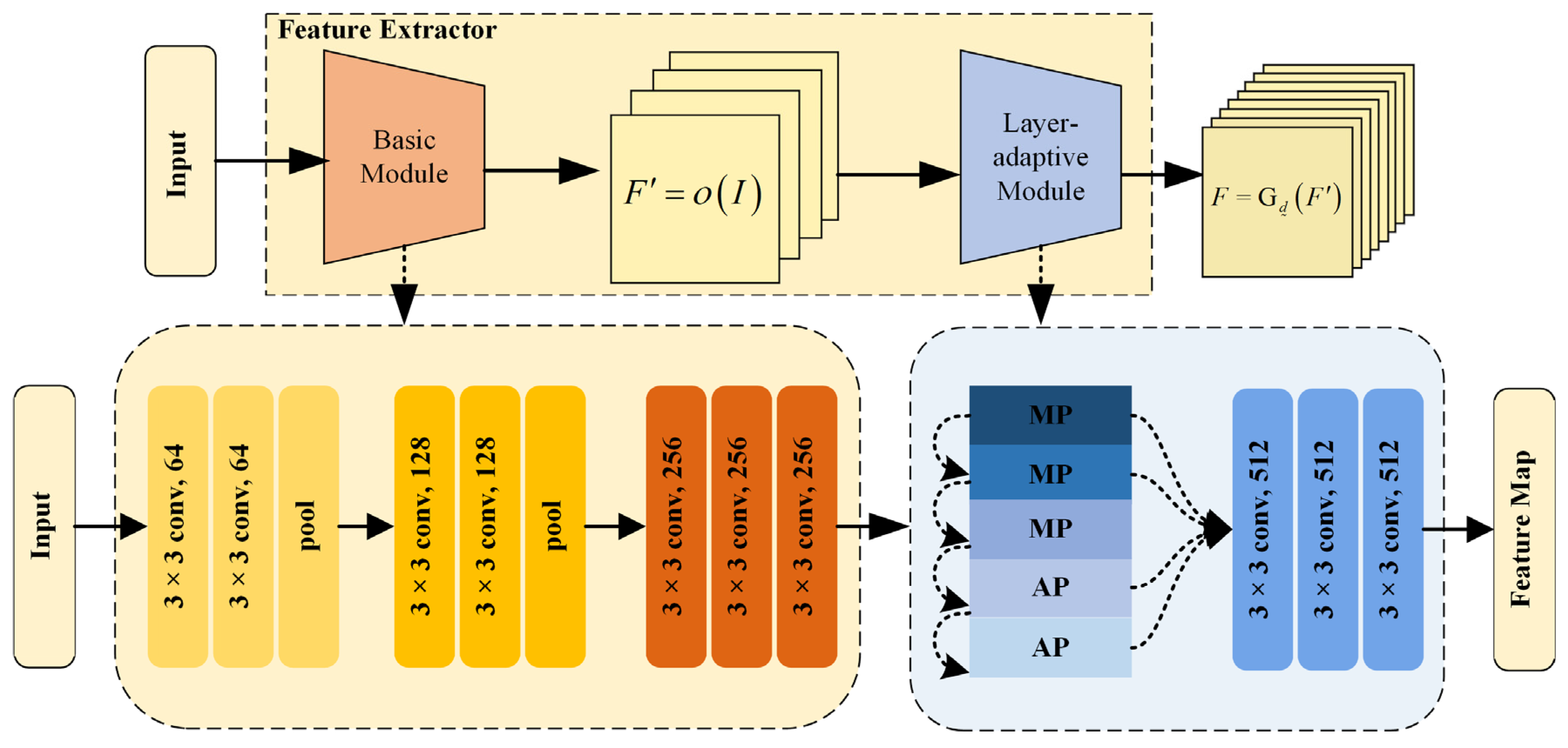
The overall flow of the proposed method is as follows: First, the CNN network is used for feature extraction of RSIs from different sources. The proposed CNN-based feature extraction network consists of a basic module and a layer-adaptive module. The network structure and parameters in the basic module are fixed and used for preliminary extraction of image features. The output from the basic module is further processed as an input to the layer-adaptive module. In the adaptive module, for images with different characteristics, different combinations of pooling and convolutional layers are used by initially estimating the error and giving feedback so as to obtain features more suitable for matching. After the layer-adaptive module, a 3D feature map is output. Second, feature detection and description are performed on the feature map. Key points are detected in the feature map by three different detection conditions, and the high-dimensional vectors at the corresponding position in the feature map are the descriptors of the key points. Third, Euclidean distance is used to measure the similarity between feature descriptors. A K-D tree is used for searching and obtaining candidate matching points. The final GCPs are obtained by eliminating the mismatched points using the random sample consensus (RANSAC). The framework of the proposed layer-adaptive GCPs extraction method is shown in Figure 1.

Figure 1. Framework of the proposed layer-adaptive GCPs extraction method.

3.1. CNN Feature Extractor

The GCP extraction algorithm, based on low-level features of the image, mainly relies on the gray-level gradient, contour, texture, and edge. However, the nonlinear radiation differences between heterogeneous RSIs result in the fact that these kinds of features are not shared across modes. In particular, compared with visible images, TIR images record the thermal radiation characteristics of features, and their grayscale distribution has no linear relationship with the target reflection characteristics. Additionally, due to the longer wavelength, TIR images have lower resolution, which makes edge features less obvious. Considering that the deep features reflect the semantic information of the image, a CNN-based network is used as a feature extractor in order to obtain the deep features for GCPs matching. The proposed CNN feature extractor is divided into a basic module and an adaptive module.

3.1.1. Basic Module

CNN is one of the representative algorithms of deep learning and is widely used in image classification, natural language processing, human motion prediction, target detection and recognition, etc. A typical CNN is formed by a combination of a convolutional layer, a pooling layer, and a fully connected layer. The convolutional layer performs convolution on the input image using filters with specific trainable weights to obtain a feature map. The feature maps input to the pooling layer are processed in a window with a maximum or average pooling operation, which selects the maximum or average value in the operation window as the output, respectively. Each node in the fully connected layer is connected to all nodes in the previous layer in order to map the distributed feature representation extracted from the convolutional layer to the sample label space. Here, we introduce the VGG-16 model, a classical convolutional neural network model for image classification with powerful feature extraction capabilities after being trained. The original VGG-16 network consists of thirteen convolutional layers and three fully connected layers. Here, we use conv1, conv2, and conv3 as the basic modules in our CNN feature extractor.

The basic module $\mathcal{B}$ is mainly composed of the first three convolutions of the VGG-16 network. The input of the basic module is an image $\mathrm{I}$ with a size of $a\times b$. The output feature map of the basic module $F^{\prime }=\mathcal{B}\left(I\right), F^{\prime }\in {ℝ}^{w\times h\times n}$. After the third layer of convolution, the number of feature map channels is 256, that is, $n = 256$, and the spatial resolution of the feature map becomes a quarter size of $I$ due to the pooling operation. For all input images, the basic module $\mathcal{B}$ is the same, including the organizational structure and parameters of layers. The output $F^{\prime }$ of the basic module continues to enter the adaptive module for convolutional operation. In the adaptive module, the composition and parameters of the network will be adaptively changed according to the different input images so as to extract the modal-invariant features for GCP extraction.

3.1.2. Layer-Adaptive Module

The proposed CNN network has a layer-adaptive module that can adaptively determine which features are more important and automatically select them during the sampling process. The layer-adaptive module is aimed at the target of feature point extraction and detection of remote sensing images from different sources, carries out network adaptive fine-tuning for different input images, selectively uses different types of pooling layers and their parameters, and uses the output of different convolution layers as the final output result. The infrastructure of our adaptive module consists of one pooling layer and three convolution layers. The standard operation of the pooling layer is to take the maximum value or average value according to the step size in the pooling window and then sample the feature map. The pooling layer itself has no parameters to learn, but it can reduce the size of neural network parameters, increase the receptive field, and retain significant texture features (max pooling) or global average features (average pooling). The previous neural network structures used a single pooling layer fixedly. However, when used as a feature extractor, the operation of the pooling layer, such as the selection of pooling type and the window size of the pooling operation, will have an impact on the subsequent feature extraction and control point extraction accuracy. Therefore, after the preliminary estimation of GCP extraction accuracy, we make an adaptive adjustment to the pooling layer in the adaptive module and complete the adjustment when the extraction accuracy reaches the preset threshold.

We denote the adaptive module as ${\mathcal{G}}_d,d=1,2,3,4,5$. According to Table 1, the variable $d$ assumes distinct values that correspond to various operations. The operations in the table are sorted from highest to lowest priority. The priority of each operation is determined by the empirical value obtained from the previous experiment. The smaller the value, the more likely the operation is to obtain higher accuracy in our task.

Table 1. Operations of the layer-adaptive module. The number in parentheses represents the window size and strides of the pooling operation. Conv4 includes three convolutional layers with kernel sizes of 3 × 3 × 512.

$\mathit{d}$	Operation
1	max pooling(2,1) + conv4
2	max pooling(3,1) + conv4
3	max pooling(4,1) + conv4
4	average pooling(2,1) + conv4
5	average pooling(3,1) + conv4

Define the tracking error:

$$e=R_d-R$$

(1)

where $R_{d }$ is the preliminary estimation accuracy, and $R$ is the accuracy threshold. When the GCPs accuracy is lower than the threshold accuracy, that is, $e>0$, we let $d=d+1$. The adaptive module updates and reprocesses until there is a $\tilde{d}$ making $e\le 0$. If there is still $e>0$ after all operation combinations have been tested, select ${\mathcal{G}}_{\tilde{d}},\tilde{d}=1,2,3,4,5$ that minimizes $e$. $F={\mathcal{G}}_{\tilde{d}}\left(F^{\prime }\right)$ is the output feature map of the layer-adaptive module, which is also the output of the CNN feature extractor. The schematic diagram of the whole feature extraction network is shown in Figure 2.

Figure 2. Architecture of the CNN feature extractor. AP and MP stand for average pooling and maximum pooling operations.

3.2. Feature Detection and Description

3.2.1. Feature Detection and Description on $F$

The output feature map of the CNN feature extractor is used for both feature detection and description. Here, we consider the different meanings represented by the feature map $F$: as a 3D tensor, $F$ can be considered as a set of high-dimensional vectors in the channel direction. At the same time, on a channel-by-channel basis, a feature map $F$ can be viewed as a set of 2D feature detection response maps $D^k\in {ℝ}^{h\times w}, k=1,\dots ,n$.

Combining the considerations in both directions, we use the feature map $F$ for both the detection and description of the key points [19]. When the feature map is used for detection, first the channel with the largest feature vector response is found:

$$m=\arg \underset{k}{\max }{D}^k$$

(2)

subsequently the local maximum value is detected:

$$D_{ij}^m \mathrm{is} \max \mathrm{in} D_{i^{\prime }{j}^{\prime }}^m,\left(i^{\prime },j^{\prime }\right)\in \mathcal{N}\left(i,j\right)$$

(3)

where $\mathcal{N}\left(i,j\right)$ is the set of $3\times 3$ neighbors of the pixel $\left(i,j\right)$. When (2) and (3) are satisfied at the same time, $\left(i,j\right)$ is the feature point, and the feature descriptor of this point is obtained by normalizing the 512-dimensional vector corresponding to $\left(i,j\right)$ in the feature map:

$${\widehat{d}}_{ij}=d_{ij}/{\Vert d_{ij}\Vert }_2$$

(4)

3.2.2. Multiscale Detection

The feature pyramid is a basic method used to detect objects of different sizes. Scale changes often exist between RSIs from different sources due to the influence of image resolution. Therefore, we use the image feature pyramid to obtain scale robustness features. For an input image $I$, different multiples of sampling operations are performed and input into the feature extraction network to obtain the feature pyramid:

$$P=\left\{\left.F^{\rho }\right|\rho =0.5,1,2\right\}$$

(5)

$\rho =0.5,1,2$ corresponds to different resolutions. The low-resolution feature maps in $P$ are fused [19]:

$${\tilde{F}}^{\rho }=F^{\rho }+{\displaystyle \sum _{\gamma <\rho }{F}^{\gamma }}$$

(6)

The low-resolution feature maps are upsampled for accumulation using bilinear interpolation during fusion. Detected positions are marked and upsampled from the coarsest resolution to the next scales, resulting in a marked region. The subsequent key points detected in the marked region are ignored in order to avoid redundancy detection.

3.3. Feature Matching and Outlier Removal

The distance between two instance points in the feature space is a response to the degree of similarity between the two. In this paper, we measure the similarity of two feature points based on the Euclidean distance between the feature descriptors. The Euclidean distance for two points to be matched is:

$$des\left(d,d^{\prime }\right)=\sqrt{{\displaystyle {\sum }_{i=1}^n{\left(d_i-d_i^{\prime }\right)}^2}}$$

(7)

In a collection $E$ of points to be matched, $d^{\prime }$ is the nearest neighbor of the point $d$ when:

$$\forall d^{″}\in E,des\left(d,d^{\prime }\right)\le t\cdot des\left(d,d^{″}\right)$$

(8)

When searching for the nearest neighbor of a point, a K-D tree is used to build a data index for searching and obtaining candidate matching pairs for efficiency. Finally, the RANSAC algorithm is used for outlier elimination and matching. We chose the affine transformation model to determine the geometric constraint relationship between image pairs.

3.4. Transfer Learning and Fine-Tuning

3.4.1. Transfer Learning

When used as a feature extractor, CNN is generally required to have strong generalization abilities to realize the processing of different tasks. In order to improve the generalization ability of the network, a lot of work has been carried out on the structure and optimization process of the neural network. At the same time, in deep learning, more training data means that deeper networks can be used and network generalization ability can also be improved. However, for many tasks related to RSI processing, the difficulty of data set acquisition and production has always been a problem since it takes a lot of manpower and material resources to improve the network generalization ability through large-scale data sets. In fact, in practical applications, in addition to focusing on how to enhance the generalization ability of CNN, the characteristics of tasks and data themselves are also very important. In our research, when CNN is used as a feature extractor, its mission is no longer to output image classification or image segmentation results but to output feature maps that retain important details or overall features of the image while retaining certain spatial positioning capabilities at the same time, so as to detect candidate GCPs and describe their features for matching.

For deep networks for different missions, shallow layers of networks are more likely to learn primary features that are common to all tasks, while deep networks are more relevant to their specific tasks. Therefore, we choose to fine-tune the specific layers, conv4_3, on the pre-trained network to improve the performance on feature extraction. Specifically, for a VGG-16 network pre-trained on ImageNet [30], we discard the part after conv4_3 and freeze the weights of the convolutional layers before conv4_3. We use the MegaDepth [31] dataset to fine-tune our feature extractor. In the fine-tuning process, the learning rate is set at 0.001 and divided by 2 every 10 epochs. Finally, we pick conv1, conv2, and conv3 of the trained VGG-16 as the basic modules and the rest as the layer-adaptive modules.

3.4.2. Triplet Margin Ranking Loss

Due to the fact that feature extraction networks are used for both feature detection and feature description, we focus on the following two points for network training: when detecting features, key points are repeatable under various imaging conditions. When describing features, the feature descriptors should be as unique as possible in order to facilitate subsequent matching and avoid mismatching. Considering the above two aspects, we use the triplet margin ranking loss (TMRL) [32] as the loss function. The triplet margin ranking loss for a margin $M$ can then be defined as:

$$m\left(c\right)=\max (0,M+p{\left(c\right)}^2-n{\left(c\right)}^2)$$

(9)

where $p\left(\mathrm{c}\right)$ is the positive descriptor distance between the corresponding descriptors and $n\left(\mathrm{c}\right)$ is the negative distance between them. This TMRL enhances the distinctiveness of feature descriptors by penalizing any irrelevant descriptors that lead to incorrect matching. In addition, a detection term is added to the triplet margin ranking loss in order to seek out the repeatability of detections [19]:

$$L\left(I_1, I_2\right)={\displaystyle \sum }_{c\in C}\frac{s_c^{\left(1\right)}{s}_c^{\left(2\right)}}{{{\displaystyle \sum }}_{q\in C}{s}_q^{\left(1\right)}{s}_q^{\left(2\right)}}m\left(p\left(c\right),n\left(c\right)\right)$$

(10)

where $C$ is the set of all correspondences between $I_1$ and $I_2$, and $s_c^{\left(1\right)},s_c^{\left(2\right)}$ are the detection scores [19] at points A and B in $I_1$ and $I_2$.

The above loss function will generate the weighted average value of the margin terms $\mathrm{m}$ based on the detection scores of all matches. Therefore, in order to minimize the loss, the most relevant correspondence with a lower margin term will obtain higher relative scores. In the same way, correspondences with higher relative scores are encouraged to obtain similar descriptors that are different from other features.

3.4.3. Training Data

In order for the feature extractor to learn the expression of pixel level feature similarity under the radiation and geometric differences of heterogeneous images, the selection of training data needs to meet three conditions:

• The scale of the training data should be large enough.
• Training data needs to have pixel-level correspondence.
• The training data should have significant radiation and geometric differences.

In order to meet the above conditions, we used the MegaDepth dataset. It is composed of more than 1 million landmark images with large differences in shooting light and scale. It also contains a large number of multimodal image pairs, such as day and night. The dataset screened approximately 100,000 high-quality images from these images and reconstructed 196 different scenes using the open-source motion recovery structure software COLMAP [33]. From these three-dimensional scenes, stereo image pairs can be obtained. For each image pair, using the 3D information and camera parameters provided, the pixels on the second image can be projected onto the first image, establishing pixel-level correspondence between the image pairs, which satisfies the second condition we provide. Thus, the MegaDepth dataset satisfies the above three conditions and is selected for model training.

4. Experimental Results and Discussion

To verify the effectiveness of the proposed method, we selected several infrared RSIs for evaluation. We compare our method against SIFT, RIFT, and D2-Net. The program is executed on a workstation with an Intel Xeon(R) Gold 6248R CPU running at 3.00 GHz, 376 GB of RAM, and an NVIDIA A100 GPU. The operating system is Ubuntu20.04. The code is programmed in MATLAB and Python 3.7.

4.1. Experimental Datasets

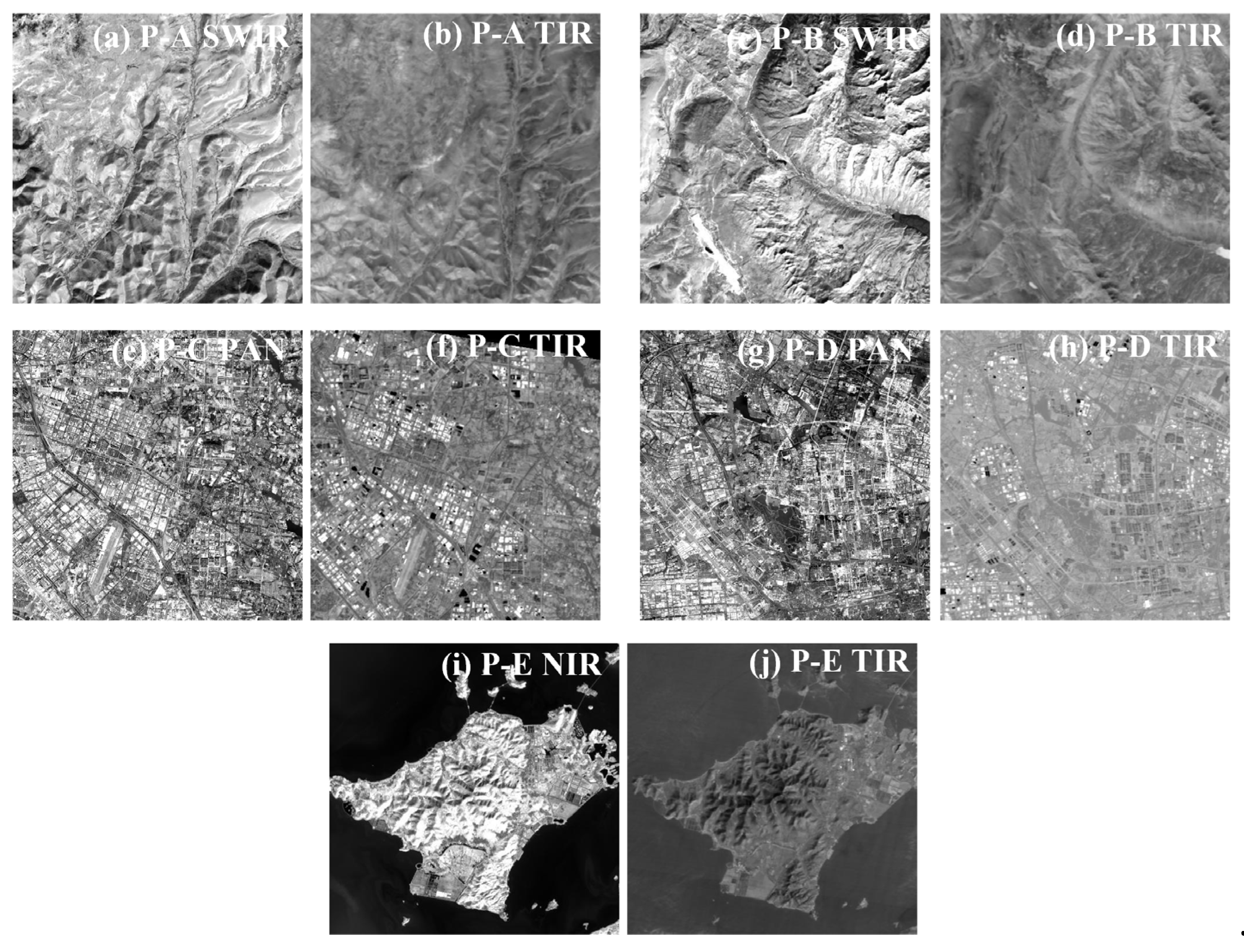
SDGSAT-1 TIS has an unprecedented infrared imaging capability, which can provide TIR images with a high spatial resolution of 30 m. Landsat 8 OLI provides PAN images at a spatial resolution of 15 m and SWIR and NIR images at 30 m. We selected images from SDGSAT-1 and Landsat 8 OLI to test the proposed method. The selected images include different scenes, such as mountain areas and urban areas, with a time span from 2013 to 2022. The details of the test data are introduced in Table 2. Figure 3 shows all the test data.

Table 2. Introduction of test data.

Item	Satellite	Category	Date and Time (Local)	Bands (μm)	GSD 1 (m)	Description
P-A and P-B	Landsat-8 OLI	SWIR	3 February 2021, 11:45	2.1–2.3	30	Mountainous areas
	SDGSAT-1-TIS	TIR	20 November 2022, 14:36	8.0–10.5	30
P-C and P-D	Landsat-8 OLI	PAN	30 January 2021, 10:32	0.50–0.68	15	Dense urban distribution areas
	SDGSAT-1-TIS	TIR	24 February 2022, 09:45	10.3–11.3	30
P-E	Landsat-8 OLI	NIR	10 December 2013, 10:32	0.84–0.88	30	Large span of time, containing waters
	SDGSAT-1-TIS	TIR	24 February 2022, 09:45	10.3–11.3	30

¹ GSD refers to Ground Sample Distance.

Figure 3. Test datasets. The size of all the SWIR, NIR, and TIR images is 500 × 500, and the size of the PAN images is 1000 × 1000.

4.2. Results and Discussion

4.2.1. Experiment 1

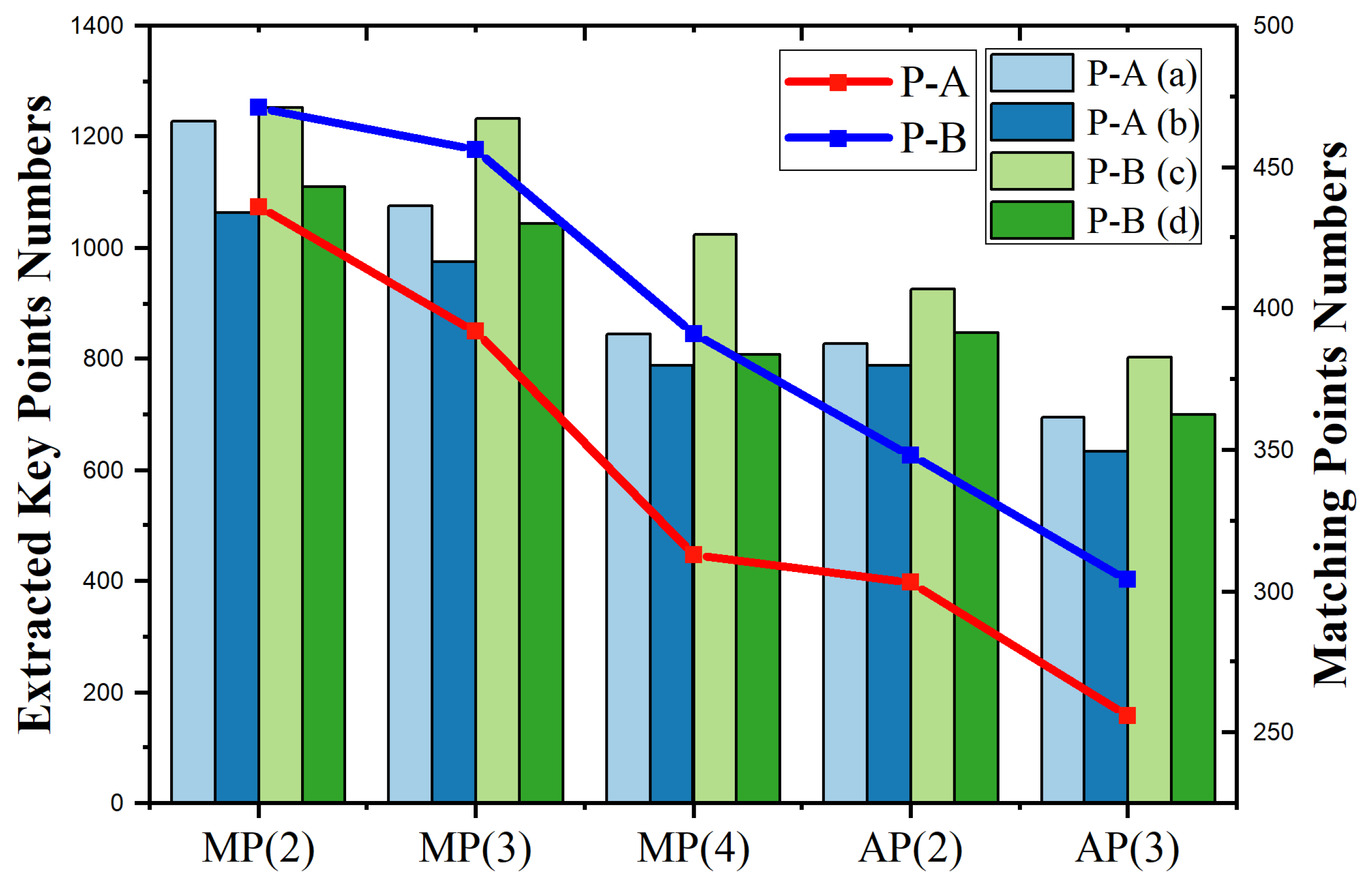
In order to explain the impact of different pooling operations and the reasons for the coding sequence of the layer-adaptive module, we count the number of key points that can be detected in the output feature map and the number of correct matching points when using different pooling operations. As shown in Figure 4, it can be seen that when the max pooling layer with a window size 2, which corresponds to the adaptive module ${\mathcal{G}}_1$ is adopted, the largest number of key points and the number of final correct matching points can be obtained. Therefore, the module with max pooling and core size 2 has the highest priority. These are the reasons for the priority of different operations in the adaptive module.

Figure 4. The number of key points extracted from the feature map and the number of correct matching key points when different pooling operations and parameters are used. MP in the horizontal coordinates represents maximum pooling, AP represents average pooling, and the number in parentheses represents the pooling window size. The bar chart indicates the number of key points extracted from the feature map, and the line chart indicates the number of correct matches obtained.

4.2.2. Experiment 2

For the purpose of performance evaluation, root-mean-square error (RMSE), the number of GCPs (NGCPs), and running time (RT) are adopted to make the analysis. We introduce RMSE to evaluate the accuracy of GCP extraction as:

$$RMSE=\sqrt{\frac{1}{N}{\displaystyle \sum _{i=1}^N\left[{\left(x_i^{\prime }-x_i\right)}^2+{\left(y_i^{\prime }-y_i\right)}^2\right]}}$$

(11)

where $\left(x_i,y_i\right)$ and $\left(x_i^{\prime },y_i^{\prime }\right)$ are the coordinates of GCPs in the sensed and referenced images under the UTM reference system, respectively. The robustness of the extraction method when dealing with images from different scenes can be evaluated by NGCPs. When the accuracy of the extracted GCPs is basically the same, a larger NGCP means a larger number of available GCPs, and the alignment accuracy becomes higher when using the GCPs for applications such as geometric correction. RT is a simple and direct index to measure the speed of a GCP extraction method, which reflects the efficiency of the method.

We select SWIR, PAN, and NIR images with TIS images for GCP extraction experiments. The test datasets have different wavebands, scales, and resolutions, including a variety of scenes such as mountainous areas, cities, and waters, a large time span, and different degrees of NDR. Table 3 shows the results of SIFT, RIFT, D2-Net, and the proposed method.

Table 3. Comparison of the results of different GCP extraction methods. ‘-’ represents RMSE > 5 pixels.

Item	Method	RMSE (Pixel)	NGCPs	RT (s)	Item	Method	RMSE (Pixel)	NGCPs	RT (s)
P-A	SIFT	-	7	0.493	P-B	SIFT	-	8	0.753
	RIFT	1.528	350	13.11		RIFT	1.501	296	13.45
	D2-Net	1.309	503	5.016		D2-Net	1.400	337	4.259
	Proposed (R = 0.8)	0.737	622	5.515		Proposed (R = 0.8)	0.749	561	5.111
P-C	SIFT	-	5	0.541	P-D	SIFT	-	4	0.525
	RIFT	4.389	248	12.87		RIFT	4.023	217	12.51
	D2-Net	0.417	2735	8.159		D2-Net	0.664	1798	9.422
	Proposed (R = 0.2)	0.088	6644	12.56		Proposed (R = 0.2)	0.132	4181	11.554
P-E	SIFT	1.003	36	0.446
	RIFT	1.002	1397	13.6
	D2-Net	1.224	819	3.316
	Proposed (R = 0.8)	0.791	1069	3.453

As shown, the SIFT algorithm fails on P-A, P-B, P-C, and P-D because of low resolution and severe NDR, as well as different scales. The reason SIFT succeeds in P-E is because of the presence of clear and significant edge features in P-E. Furthermore, the characteristics of relatively small image information lead to good results in P-E not only for SIFT but also for the remaining three methods. However, the NGCP of SIFT is small even when the matching is successful, i.e., 36.

RIFT can obtain a GCP extraction accuracy of 1.5 pixels on average and a certain number of GCPs in P-A, P-B, and P-D. It is worth noting that RIFT is not scale invariant; therefore, for P-C and P-D, the two images of each image pair need to be resampled to have approximately the same GSD [17]. However, after adjusting the TIS image using bilinear interpolation, the RMSEs of RIFT in both P-C and P-D reach 4 pixels, which may be due to the fact that our resampling method is not suitable enough. The analysis above reflects the drawback of the RIFT method, which is its lack of robustness at scale. Additionally, the RIFT method takes relatively longer due to the fact that the RIFT algorithm needs to compute the maximum index map constructed from the log-Gabor convolution sequence for feature description, which is time-consuming.

D2-Net and our proposed method are all based on CNN and use deep features for matching. Since the semantic information is not disturbed by radiation differences, it can be seen that both methods using deep features are robust in different experimental scenarios, which indicates that the deep-learning-based method is suitable for heterologous RSI and GCP extraction. In P-A, P-B, and P-E involving TIR, NIR, and SWIR images, the D2-Net method achieved an average RMSE of 1.5 pixels and an average run time of about 3–4 s. In P-C and P-D images, including panchromatic and TIR images, the D2-Net method achieves an accuracy of 0.5 pixels, but with a higher time cost.

The proposed method is superior in accuracy and NGCPs to the other three methods. The RMSE of TIS images with SWIR and NIR images could reach 0.8 pixels, and an even higher accuracy of 0.1 pixels could be reached between TIS and PAN images. The reasons are as follows: (1) The proposed method is accuracy-oriented, adding feedback and adaptive adjustment mechanisms based on a given error threshold, always tending to obtain the most accurate extraction results. (2) In a general sense, the higher the number of key points that can be initially extracted from the output feature map, the higher the number of GCPs that can be subsequently filtered to meet the accuracy requirement. As a result, our method also always tends to obtain a larger number of GCPs, i.e., larger NGCPs. However, it should be noted that our method is not optimal in terms of run time. This is because during the adjustment performed by the layer-adaptive module, the accuracy of the point extraction needs to be initially estimated, which leads to the possibility that more time is needed for the computation. That is, our method tends to trade off runtime for a more accurate result.

In general, our method is able to extract sub-pixel-level GCPs for TIR images with low resolution. Furthermore, when higher resolution images are available for reference, such as panchromatic images in P-C and P-D, our method can obtain high precision GCPs with RMSEs around 0.1, which is crucial for subsequent quantification applications of remote sensing images.

Figure 5 shows the results of the four methods on the datasets. As seen, SIFT fails in all datasets except P-E. It is clear that the proposed method could basically obtain the largest number of GCPs and the most uniform distribution of GCPs. RIFT obtains relatively more GCPs in P-E. Compared to our proposed method, D2-Net performs slightly inferiorly because the network of D2-Net is fixed.

Figure 5. The results of four methods. The red lines and the yellow lines indicate the correct matches and the outliers, respectively.

4.3. Further Evaluation and Analysis

4.3.1. Ablation Study

In this paper, we propose a layer-adaptive module to obtain features that are more suitable for matching and improve the accuracy of GCP extraction. We also perform resampling before inputting the image into the feature extraction network to improve robustness for images of different scales. To verify the effectiveness of the layer adaptation module and resampling operation, we conducted ablation experiments. We removed the layer adaptation module and the sampling process for experiments, and the experimental results are shown in Table 4.

Table 4. Comparison of the results of the ablation study.

Item	Method	RMSE (Pixel)	NGCPs	RT (s)
P-A	Proposed (Without LAM 1)	1.324	447	3.989
	Proposed (Without Resampling)	0.918	369	2.723
	Proposed (Without LAM and Resampling)	1.871	294	2.253
	Proposed	0.737	622	5.515
P-B	Proposed (Without LAM)	1.531	430	3.408
	Proposed (Without Resampling)	0.985	237	2.662
	Proposed (Without LAM and Resampling)	1.537	233	2.708
	Proposed	0.749	561	5.111
P-C	Proposed (Without LAM)	0.484	2030	5.632
	Proposed (Without Resampling)	0.889	414	9.571
	Proposed (Without LAM and Resampling)	1.049	297	3.444
	Proposed	0.088	6644	12.56
P-D	Proposed (Without LAM)	0.463	1087	5.463
	Proposed (Without Resampling)	0.148	498	9.583
	Proposed (Without LAM and Resampling)	0.791	383	3.512
	Proposed	0.132	4181	11.554
P-E	Proposed (Without LAM)	1.121	925	3.416
	Proposed (Without Resampling)	0.917	572	2.676
	Proposed (Without LAM and Resampling)	1.075	561	2.676
	Proposed	0.791	1069	3.453

¹ LAM refers to the layer-adaptive module.

From the experimental results, it can be seen that the RMSE of GCPs significantly increases and the accuracy decreases after removing the layer-adaptive module. This indicates that the features extracted by the layer-adaptive module are more suitable for our matching task. In addition, for test groups P-C and P-D with scale differences, the number of GCPs detected significantly decreased after removing the resample operation, which indicates that this operation makes the proposed method robust to scale changes.

4.3.2. Model Complexity Analysis

Larger input data and more complex networks will lead to a greater consumption of computing resources. We compare the complexity and computational cost of the proposed model with other deep learning-based methods. From Table 5, it can be seen that our proposed method has a relatively small number of parameters. This is because in the layer adaptation module, the adjustment mainly relies on the role of different pooling layers, and the pooling layers themselves do not have weight parameters, which helps the model be lightweight. In addition, our model does not include fully connected layers involving large-scale parameters, which is one of the reasons why the model parameters are relatively small. In terms of computational cost, compared to large-scale classification networks, our computing cost has decreased due to the fact that, although our backbone network is based on VGG-16, we have abandoned all layers behind conv4_3, which reduces a significant amount of convolutional operations and computational costs in our network.

Table 5. Parameters and GFLOPs of different GCP extraction models.

Model	Image Size	GFLOPs	Parameters
VGG16	224	15.5	138 M
ResNet-based	224	3.87	25.6 M
VGG16-based	224	14.4	9.99 M
DenseNet-based	224	11.32	7.89 M
Proposed	224	13.9	7.63 M

4.3.3. Discussion

Overfitting is a common problem in machine learning. While our method obtains good results, it is also necessary to discuss whether there is an overfitting problem in the model. Here, we give two reasons to support the claim that our results are not caused by overfitting. Firstly, there is no overlap between our training data and the test data used in the experiment. During the training process, we used a large-scale universal dataset, i.e., MegaDepth. In previous work, a common approach was to match RSIs and capture image blocks that corresponded in pixels to the dataset, and then expand the dataset for training through data augmentation. However, although the dataset we use conforms to the one-to-one correspondence between pixels and meets the requirements of multimodal images, it is not a remote sensing image dataset. In fact, MegaDepth is a more general and large-scale image dataset. After training on this data set, if the model is overfitting, it will not produce good results in our test data, i.e., heterologous RSIs. The test results in Experiment 2 demonstrate that our model has strong generalization ability and has achieved good results on the test data. In addition, we used the method of transfer learning. Our network only fine-tunes the conv4_3 on the network that is pretrained on ImageNet. In the process of fine-tuning, all weights except conv4_3 are frozen, which means the parameters of the shallow layers will not change completely depending on the training data set, thus avoiding overfitting in the training process.

The proposed method has achieved high accuracy in GCPs, but there are still some shortcomings. Firstly, the appropriate selection of accuracy thresholds is a topic worth discussing. The characteristics of our proposed method require us to provide an accuracy threshold before extracting control points, and subsequent adaptive adjustment operations will be based on the preset threshold. If the accuracy threshold is set too low at the beginning, it will cause the adaptive module to make multiple adjustments to achieve the target accuracy, which will consume relatively more time. Similarly, setting the accuracy threshold too high can also lead to poor accuracy in the final result. Secondly, currently, our method is relatively semi-intelligent, essentially replacing the features used for matching in traditional methods with deep features. Thirdly, in the detection phase, we only considered using the feature maps output from the last convolutional layer and ignored the outputs of other layers.

In future work, it can be considered to establish mapping relationships with different adaptive modules based on calculating some statistical values of the input image in order to avoid potential resource waste caused by the iterative process. In addition, it is possible to consider researching an end-to-end network that can directly output the final control point extraction results. In addition, it is also possible to consider combining feature maps output from other convolutional layers for joint detection, utilizing the higher spatial resolution of low-level feature maps to improve the positioning accuracy of points.

5. Conclusions

In this paper, we propose a CNN-based layer-adaptive GCP extraction method for TIR RSIs that can improve the accuracy of GCPs. The proposed network can adaptively use different pooling layers to obtain features more suitable for matching. The proposed method is robust to NRD between heterologous RSIs, which makes it outperform previous intensity-based or feature-based methods. The method is tested on various scenes from SDGSAT-1-TIS images and Landsat-8 OLI SWIR, PAN, and NIR images. The experimental results show that this method improves the accuracy of GCP extraction from TIR RSIs.

References

1. Jiang, L.Y.; Li, L.Y.; Li, X.Y.; Jiao, J.J.; Chen, F.S. Extrapolating distortion correction with local measurements for space-based multi-module splicing large-format infrared cameras. Opt. Express 2022, 30, 38043–38059. [Google Scholar] [CrossRef] [PubMed]
2. Yang, L.; Li, X.Y.; Jiang, L.Y.; Zeng, F.J.; Pan, W.H.; Chen, F.S. Resolution-Normalizing Image Stitching for Long-Linear-Array and Wide-Swath Whiskbroom Payloads. IEEE Geosci. Remote Sens. Lett. 2022, 19, 7507705. [Google Scholar] [CrossRef]
3. Li, X.Y.; Hu, Z.Y.; Jiang, L.Y.; Yang, L.; Chen, F.S. GCPs Extraction with Geometric Texture Pattern for Thermal Infrared Remote Sensing Images. IEEE Geosci. Remote Sens. Lett. 2022, 19, 7000205. [Google Scholar] [CrossRef]
4. Maes, F.; Collignon, A.; Vandermeulen, D.; Marchal, G.; Suetens, P. Multimodality image registration by maximization of mutual information. IEEE Trans. Med. Imaging 1997, 16, 187–198. [Google Scholar] [CrossRef] [PubMed]
5. Cole-Rhodes, A.A.; Johnson, K.L.; LeMoigne, J.; Zavorin, I. Multiresolution registration of remote sensing imagery by optimization of mutual information using a stochastic gradient. IEEE Trans. Image Process. 2003, 12, 1495–1511. [Google Scholar] [CrossRef] [PubMed]
6. Fischler, M.A.; Bolles, R.C. Random Sample Consensus—A Paradigm for Model-Fitting with Applications to Image-Analysis and Automated Cartography. Commun. ACM 1981, 24, 381–395. [Google Scholar] [CrossRef]
7. Lowe, D.G. Distinctive image features from scale-invariant keypoints. Int. J. Comput. Vis. 2004, 60, 91–110. [Google Scholar] [CrossRef]
8. Harris, C.; Stephens, M. A combined corner and edge detector. In Alvey Vision Conference; Alvety Vision Club: Manchester, UK, 1988. [Google Scholar]
9. Moravec, H.P. Obstacle Avoidance and Navigation in the Real World by a Seeing Robot Rover. Ph.D. Dissertation, Stanford University, Stanford, CA, USA, 1980. [Google Scholar]
10. Rosten, E.; Drummond, T. Fusing points and lines for high performance tracking. In Proceedings of the 10th IEEE International Conference on Computer Vision, Beijing, China, 17–20 October 2005. [Google Scholar]
11. Smith, S.M.; Brady, J.M. SUSAN—A new approach to low level image processing. Int. J. Comput. Vis. 1997, 23, 45–78. [Google Scholar] [CrossRef]
12. Chen, B.Y.; Li, X.Y.; Zhang, G.X.; Guo, Q.; Wu, Y.P.; Wang, B.Y.; Chen, F.S. On-orbit installation matrix calibration and its application on AGRI of FY-4A. J. Appl. Remote Sens. 2020, 14, 024507. [Google Scholar] [CrossRef]
13. Bay, H.; Tuytelaars, T.; Van Gool, L. SURF: Speeded up robust features. In Proceedings of the 9th European Conference on Computer Vision, Graz, Austria, 7–13 May 2006; pp. 404–417. [Google Scholar]
14. Yu, G.S.; Morel, J.M. ASIFT: An Algorithm for Fully Affine Invariant Comparison. Image Process. Line 2011, 1, 11–38. [Google Scholar] [CrossRef]
15. Ma, W.P.; Wen, Z.L.; Wu, Y.; Jiao, L.C.; Gong, M.G.; Zheng, Y.F.; Liu, L. Remote Sensing Image Registration with Modified SIFT and Enhanced Feature Matching. IEEE Geosci. Remote Sens. Lett. 2017, 14, 3–7. [Google Scholar] [CrossRef]
16. Ye, Y.; Shen, L. HOPC: A Novel Similarity Metric Based on Geometric Structural Properties for Multi-Modal Remote Sensing Image Matching. In Proceedings of the 23rd ISPRS Congress, Prague, Czech Republic, 12–19 July 2016; pp. 9–16. [Google Scholar]
17. Li, J.Y.; Hu, Q.W.; Ai, M.Y. RIFT: Multi-Modal Image Matching Based on Radiation-Variation Insensitive Feature Transform. IEEE Trans. Image Process. 2020, 29, 3296–3310. [Google Scholar] [CrossRef] [PubMed]
18. Han, X.F.; Leung, T.; Jia, Y.Q.; Sukthankar, R.; Berg, A.C. MatchNet: Unifying Feature and Metric Learning for Patch-Based Matching. In Proceedings of the IEEE Conference on Computer Vision and Pattern Recognition, Boston, MA, USA, 7–12 June 2015; pp. 3279–3286. [Google Scholar]
19. Dusmanu, M.; Rocco, I.; Pajdla, T.; Pollefeys, M.; Sivic, J.; Torii, A.; Sattler, T. D2-Net: A Trainable CNN for Joint Description and Detection of Local Features. In Proceedings of the 32nd IEEE/CVF Conference on Computer Vision and Pattern Recognition, Long Beach, CA, USA, 16–20 June 2019; pp. 8084–8093. [Google Scholar]
20. DeTone, D.; Malisiewicz, T.; Rabinovich, A. SuperPoint: Self-Supervised Interest Point Detection and Description. In Proceedings of the 2018 IEEE/CVF Conference on Computer Vision and Pattern Recognition, Salt Lake City, UT, USA, 18–22 June 2018; pp. 337–349. [Google Scholar]
21. Zagoruyko, S.; Komodakis, N. Learning to Compare Image Patches via Convolutional Neural Networks. In Proceedings of the 2015 IEEE Conference on Computer Vision and Pattern Recognition, Boston, MA, USA, 7–12 June 2015; pp. 4353–4361. [Google Scholar]
22. Krizhevsky, A.; Sutskever, I.; Hinton, G.E. ImageNet Classification with Deep Convolutional Neural Networks. Commun. ACM 2017, 60, 84–90. [Google Scholar] [CrossRef]
23. Yang, Z.Q.; Dan, T.T.; Yang, Y. Multi-Temporal Remote Sensing Image Registration Using Deep Convolutional Features. IEEE Access 2018, 6, 38544–38555. [Google Scholar] [CrossRef]
24. Ma, W.P.; Zhang, J.; Wu, Y.; Jiao, L.C.; Zhu, H.; Zhao, W. A Novel Two-Step Registration Method for Remote Sensing Images Based on Deep and Local Features. IEEE Trans. Geosci. Remote Sens. 2019, 57, 4834–4843. [Google Scholar] [CrossRef]
25. Ye, F.M.; Su, Y.F.; Xiao, H.; Zhao, X.Q.; Min, W.D. Remote Sensing Image Registration Using Convolutional Neural Network Features. IEEE Geosci. Remote Sens. Lett. 2018, 15, 232–236. [Google Scholar] [CrossRef]
26. Zhu, H.; Jiao, L.C.; Ma, W.P.; Liu, F.; Zhao, W. A Novel Neural Network for Remote Sensing Image Matching. IEEE Trans. Neural Netw. Learn. Syst. 2019, 30, 2853–2865. [Google Scholar] [CrossRef] [PubMed]
27. Hughes, L.H.; Schmitt, M.; Mou, L.C.; Wang, Y.Y.; Zhu, X.X. Identifying Corresponding Patches in SAR and Optical Images with a Pseudo-Siamese CNN. IEEE Geosci. Remote Sens. Lett. 2018, 15, 784–788. [Google Scholar] [CrossRef]
28. Zhang, H.; Ni, W.P.; Yan, W.D.; Xiang, D.L.; Wu, J.Z.; Yang, X.L.; Bian, H. Registration of Multimodal Remote Sensing Image Based on Deep Fully Convolutional Neural Network. IEEE J. Sel. Top. Appl. Earth Obs. Remote Sens. 2019, 12, 3028–3042. [Google Scholar] [CrossRef]
29. Simonyan, K.; Zisserman, A. Very deep convolutional networks for large-scale image recognition. In Proceedings of the International Conference on Learning Representations, San Diego, CA, USA, 7–9 May 2015. [Google Scholar]
30. Deng, J.; Dong, W.; Socher, R.; Li, L.J.; Li, K.; Li, F.F. ImageNet: A large-scale hierarchical image database. In Proceedings of the 2009 IEEE Conference on Computer Vision and Pattern Recognition, Miami Beach, FL, USA, 20–25 June 2009; pp. 248–255. [Google Scholar]
31. Li, Z.Q.; Snavely, N. MegaDepth: Learning single-view depth prediction from internet photos. In Proceedings of the 31st IEEE/CVF Conference on Computer Vision and Pattern Recognition, Salt Lake City, UT, USA, 18–23 June 2018; pp. 2041–2050. [Google Scholar]
32. Mishchuk, A.; Mishkin, D.; Radenovic, F.; Matas, J. Working hard to know your neighbor’s margins: Local descriptor learning loss. In Proceedings of the 31st Annual Conference on Neural Information Processing Systems (NIPS), Long Beach, CA, USA, 4–9 December 2017. [Google Scholar]
33. Schonberger, J.L.; Frahm, J.M. Structure-from-Motion Revisited. In Proceedings of the 2016 IEEE Conference on Computer Vision and Pattern Recognition (CVPR), Seattle, WA, USA, 27–30 June 2016. [Google Scholar]
Disclaimer/Publisher’s Note: The statements, opinions and data contained in all publications are solely those of the individual author(s) and contributor(s) and not of MDPI and/or the editor(s). MDPI and/or the editor(s) disclaim responsibility for any injury to people or property resulting from any ideas, methods, instructions or products referred to in the content.
Article Metrics
Citations
Article Access Statistics
Multiple requests from the same IP address are counted as one view.