Article

How Many Reindeer? UAV Surveys as an Alternative to Helicopter or Ground Surveys for Estimating Population Abundance in Open Landscapes

by
Ingrid Marie Garfelt Paulsen
1,*,†,
Åshild Ønvik Pedersen
1,†,
Richard Hann
2,
Marie-Anne Blanchet
1,
Isabell Eischeid
1,3,
Charlotte van Hazendonk
4,
Virve Tuulia Ravolainen
1,
Audun Stien
3 and
Mathilde Le Moullec
5
1
Norwegian Polar Institute, Fram Centre, 9296 Tromsø, Norway
2
Department of Engineering Cybernetics, Norwegian University of Science and Technology, 7491 Trondheim, Norway
3
Department of Arctic and Marine Biology, UiT—The Arctic University of Norway, 9037 Tromsø, Norway
4
Department of Arctic Geophysics, University Centre in Svalbard (UNIS), 9171 Longyearbyen, Norway
5
Centre for Biodiversity Dynamics, Department of Biology, Norwegian University of Science and Technology, 7491 Trondheim, Norway
*
Author to whom correspondence should be addressed.
These authors contributed equally to this work.
Remote Sens. 2023, 15(1), 9; https://doi.org/10.3390/rs15010009
Submission received: 10 October 2022 / Revised: 7 December 2022 / Accepted: 13 December 2022 / Published: 20 December 2022

Abstract

:
Conservation of wildlife depends on precise and unbiased knowledge on the abundance and distribution of species. It is challenging to choose appropriate methods to obtain a sufficiently high detectability and spatial coverage matching the species characteristics and spatiotemporal use of the landscape. In remote regions, such as in the Arctic, monitoring efforts are often resource-intensive and there is a need for cheap and precise alternative methods. Here, we compare an uncrewed aerial vehicle (UAV; quadcopter) pilot survey of the non-gregarious Svalbard reindeer to traditional population abundance surveys from ground and helicopter to investigate whether UAVs can be an efficient alternative technology. We found that the UAV survey underestimated reindeer abundance compared to the traditional abundance surveys when used at management relevant spatial scales. Observer variation in reindeer detection on UAV imagery was influenced by the RGB greenness index and mean blue channel. In future studies, we suggest testing long-range fixed-wing UAVs to increase the sample size of reindeer and area coverage and incorporate detection probability in animal density models from UAV imagery. In addition, we encourage focus on more efficient post-processing techniques, including automatic animal object identification with machine learning and analytical methods that account for uncertainties.

1. Introduction

The distribution and abundance of species are key parameters for conservation and management of wildlife [1]. Yet, it remains challenging to estimate population size with high precision and low bias (i.e., accuracy [2]) at relevant spatial scales [3]. There are numerous methods to estimate wildlife abundance and density—ranging from direct population counts to population indices proportional to the true population size [4,5]. Abundant and easily detectable species are commonly monitored with direct density estimation methods, which includes complete or partial census, strip transect, distance sampling or capture-recapture programs [5,6]. Recent developments in uncrewed aerial vehicles (UAVs) technology open new opportunities to survey animal populations as a replacement or supplement to traditional survey techniques [7]. UAVs offer several advantages compared to traditional aerial or ground surveys (e.g., cost effectiveness, reduced environmental impact and disturbance, and operational range [8,9]), however, whether UAV methods have improved accuracy and are more efficient than traditional survey methods is largely unknown (but see [10,11]).
Remote wildlife populations are traditionally counted on foot or using aerial surveys from helicopters or planes depending on the species characteristics and management area of interest [5,12,13,14,15]. Aerial surveys are costly, with a high carbon footprint, and they are challenging when it comes to detectability and uncertainty estimates [16,17,18,19]. In comparison, counting on foot along a survey line is more time-consuming and can be logistically difficult in remote areas, with terrain features (e.g., river, cliffs) or, e.g., when the species is sparsely distributed. Distance sampling is a common method that can assess uncertainty in abundance surveys along such line transects [4,20]. A key assumption is that the probability of detecting an animal decreases with increasing distance from the observer. Thereafter, abundance estimates account for detection probability. Total count is a method assuming that all animals are counted without error. When conducted in a well-delimited area with information on presence/absence in sub-units, uncertainty can still be evaluated [21]. Both methodologies can be used to predict densities across larger areas [22]. For an aerial survey recording, e.g., images along a fixed transect width (i.e., strip transect from crewed aircraft or UAV flying at constant height), detection is independent of distance from the transect line. Yet, there are other factors that can influence detection of an object, such as the image quality and resolution [15]. Integrating measures of detection error within a surveyed area and identifying habitat covariates strongly correlated with the population density can greatly improve the accuracy of estimates when extrapolating density to larger spatial scales [3]. Only in the last decade, UAVs have been tested and successfully applied as a cost-effective alternative to traditional surveys to estimate abundance of wildlife, especially in gregarious species [23,24], but also for solitary animals [9,25].
In the High Arctic remote Svalbard archipelago, the wild Svalbard reindeer Rangifer tarandus platyrhynchus, is the largest resident mammalian herbivore in the terrestrial tundra ecosystem [26]. Svalbard reindeer are non-gregarious, inhabiting open landscapes and can appear in high density (>10 individuals/km2). The reindeer is subject to long-term monitoring because it is a key-species impacting tundra vegetation [27], is harvested locally by recreational hunting [28] and is sensitive to climate change [29,30]. The long-term monitoring is relying on total population counts along fixed routes on foot [21,31] or by helicopter [32,33], and capture-mark-recapture techniques (see [34]). Lately, there has been focus on quality assurance and standardisation of monitoring methods of the long-term ground total counts with distance sampling [21]. Total counts were found unbiased when compared to resighting of marked reindeer and highly precise when repeating counts. In comparison, distance sampling was also unbiased, while precision was lower than total counts, according to the number of transects and groups detected. This has enabled range-wide monitoring of Svalbard reindeer using the most appropriate methodology according to terrain characteristics [22]. Both total counts and distance sampling estimated similar abundances across Svalbard (22,615 ± 401 [±SE] and 21,079 ± 2983, respectively) and found that abundance was strongly correlated with vegetation productivity [22]. Thus, both ground total counts and distance sampling can serve as reference abundance estimates to evaluate other methodologies. Local wildlife managers (the Governor of Svalbard) have, however, annually monitored reindeer since 1998 in hunting units by total counts from helicopter, and the accuracy of these counts remain to be evaluated [32,35]. In addition, there is a desire for development of monitoring methods that reduce disturbance and lower human footprints [36], which suggests the use of UAVs [37].
In this paper, we assess the precision and detection rate of reindeer abundance from a UAV pilot survey compared to traditional ground and helicopter surveys. We compare the survey methods in the same spatial extent by developing models of estimated reindeer abundance and predicting the models over the same sampling scales using correlated habitat covariates. We test the feasibility of collecting data on reindeer abundance and variables affecting detection probability using UAVs, and investigate potential problems and pitfalls associated with aerial monitoring compared to ground-based surveys.

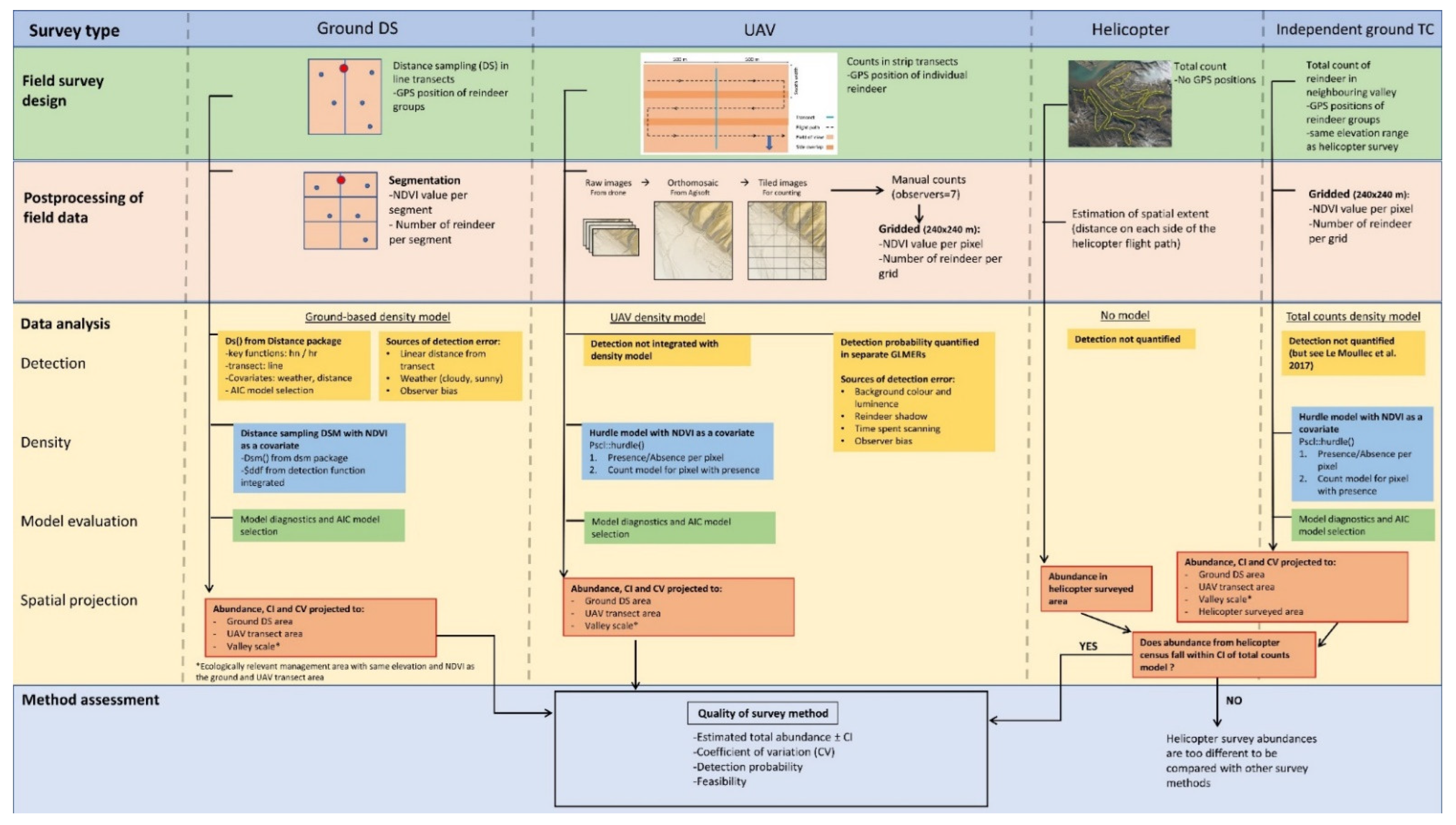
2. Materials and Methods

2.1. Study Area and Species

The Arctic Svalbard archipelago (74–81°N, 15–30°E), Norway, measures around 62,700 km2, with approximately 60% covered by glaciers, 25% by barren rocks and only 15% by vegetation [38]. We conducted the study in Sassendalen, one of the largest valleys in Central Spitsbergen (Figure 1). The valley is surrounded by peaks up to 1200 m.a.s.l. and dominated by a large river and continuous vegetation cover with wetland, ridges, and heath present only in the valley bottoms and on the lower parts of the mountain slopes (<250 m.a.s.l.) [38,39,40].
The Svalbard reindeer is distributed across all non-glaciated land areas of the archipelago. They appear mostly solitary and virtually free from predation, although rare attacks by polar bears (Ursus maritimus) have been observed [41,42]. Direct density dependence and large annual variations in weather conditions—notably the amount of rain in winter, but also the length of the snow-free season in the autumn—shape vital rates of the reindeer [29,34,43,44]. This, in turn, causes large annual fluctuations in population abundances [33,34]. Reindeer densities min the main valleys in Nordenskiöld Land are strongly synchronised due to these weather conditions, leading to spatially autocorrelated survival and mortality rates, and thus abundances [29]. This led us to assume similar population dynamics and thereby densities between the adjacent valleys.

2.2. Field Data Collection

Reindeer data were collected by four survey methodologies: (1) Ground-based distance sampling (hereafter ‘ground DS’), which served as reference to assess accuracy of the other methods, (2) UAV strip transects, (3) helicopter total counts and, (4) ground total counts from the neighbouring valley (hereafter ‘independent ground TC’) to test if extrapolations can replace the need for aerial surveys (i.e., helicopter and UAV). See Figure 2 for an illustration of the workflow.
The UAV and DS surveys were conducted on the same transects (see below) during 14–17 July 2021, but 1 day apart to reduce potential disturbance of reindeer by observers. The helicopter survey was conducted one week prior to the UAV and DS surveys (6 July) and was part of an annual census of reindeer in the valleys on Nordenskiöld Land by the Governor of Svalbard (Figure 1). Because the helicopter survey lacked positional information of individual reindeer, but densities and spatial distribution of reindeer in neighboring valleys are expected to be similar, we used the independent ground TC from the adjacent valley (Appendix A), conducted during 30 June–7 July 2021.

2.2.1. Ground Distance Sampling Survey

We followed the DS survey protocols described by [21,22] for estimating abundance of Svalbard reindeer. We allocated 10 transect lines in north–south direction, from the mountain foothills to the riverbanks, on each side of the main river in Sassendalen (Figure 1). We chose one random latitude for the first line and placed additional parallel transect lines systematically apart 2.5 km east or west from this latitude to avoid overlapping reindeer observations and to avoid violation of the assumption of independence [20]. We chose this systematic orientation across the valley (i.e., river bed to mountain side or vice versa) to reduce any bias from potential gradients in animal density related to, e.g., plant phenology and/or habitat configuration [45]. The length of each transect varied depending on the length from the mountain side to the riverbank (1.2 km to 2.9 km). All transects were walked by one observer (the same main observer as in [21,22]) at a constant speed (2–3 km h−1) without stopping, except during measurements. A handheld GPS and a compass were used to keep the line direction, and single reindeer or clusters were detected on both sides of the transect line with the naked eye. To follow the assumption of constant detection along the transect line, no scanning for reindeer was done when stopping to take measurements. Each observation was measured by laser binoculars (10 × 42 Leica Geovid, Wetzlar, Germania) to the nearest metre and a compass was used to measure the angle from the observer to the reindeer (Figure 1). For practical reasons when using the laser, measurements were taken to the largest reindeer (e.g., a mother rather than her calf) or the middle individual of a group of adults. The geographic position of the observer in the transect was also recorded. The positions of reindeer individuals/groups and perpendicular distances to the line were calculated and used in the final dataset.

2.2.2. UAV Survey

Six out of the ten line transects were mapped by an off-the-shelf DJI Mavic 2 Enterprise drone, equipped with a zoomable (24–48 mm) RGB camera. Flight plans for each line transect were prepared pre-flight with a commercial mapping software (DJIFlightPlanner, ver. 2.13). The flight plans were flown automatically with flight altitude 110–120 m above ground with a nadir (downward-looking) orientation of the camera. Test flights with different altitudes (e.g., 20–120 m) were performed before the survey to verify that reindeer could be detected on images at that height and to ensure that reindeer were minimally disturbed. At this altitude, the widest field of view (i.e., 24 mm) was used, giving a theoretical ground sample distance (GSD) of 4.4 cm and a swath width of 174 m. Side overlap was chosen with 65% and the nominal forward overlap with 85%. All lines had a run separation of 61 m and ran in an east–west direction. Ground speed was set to maximum 30 km/h and pictures taken with a frame rate of 2 s. The camera settings were on auto, but it was ensured that the shutter speed would not exceed 1/200 to prevent motion blur (max. shutter speed = GSD/ground speed), otherwise flight velocity was reduced. The total mapped area width covered 500 m on each side of the transect line. The total length of the mapping flight lines was between 20–40 km and typically took between 2–4 batteries to cover.

2.2.3. Helicopter Survey

Reindeer were counted by four observers (two pilots and two observers) in a Super Puma helicopter flying 60–100 m above the ground according to protocols by the Governor of Svalbard [32]. The flight paths (Figure 1) were assumed to cover the most important reindeer summer habitats in the Sassendalen hunting unit (see for a map of hunting units). The spatial extent of the helicopter surveyed area was defined as the entire flat valley bottom of Sassendalen and a buffer of 1 km (500 m on either side of the helicopter) around the flight routes (216 km). The census provides a single total count of all the individuals encountered, classified as calf, female/young and male, without any information on location of each animal.

2.2.4. Independent Total Counts Survey

Total counts followed the protocols described by [21,22] and were conducted in Adventdalen, the neighboring valley. Five observers walked separate predefined routes (~1 km apart from each other), scanning the entire area with 10 × 42 mm binoculars for reindeer. During the count, reindeer were categorised by age as calves, yearlings, or adults (≥2 years old) based on body size and antler characteristics. The geographic position of individual reindeer or groups were noted. At this time of the year, reindeer still have parts of their winter fur, making them conspicuous against the open tundra landscape.

2.3. Data Analyses

We estimated reindeer abundance based on field data from the survey methods of ground DS, UAV, and independent ground TC, as detailed below. Note that the helicopter total count was a single value with no data analysis. To compare estimates, we developed density spatial models (DSM) for each method as a function of vegetation productivity (Figure 2). Reindeer densities in summer correlate with vegetation productivity, as expressed by the vegetation productivity index ‘maximum normalised difference vegetation index’ (maxNDVI) [22,46]. Due to this relationship, maxNDVI was used as the common denominator to project the DSMs onto the same spatial extents in this study. The vegetation productivity layer was calculated by averaging the maxNDVI values from MODIS-satellites (Jacksonville, FL, USA) for the last five years (2017–2021) and then resampled to resolution 240 × 240 m. We used average maxNDVI because cloud coverage and random variation can affect the timing of NDVI contributing to high between-year variation [47,48]. The statistical models were adapted from Le Moullec et al. [21,22]. We fitted all models in R version 1.4.1717 [49].

2.3.1. Ground Distance Sampling DSM

The ground DS consisted of a two-stage approach with a detection probability estimation and a DSM accounting for the imperfect detection [20]. To prepare the data, we divided the transect lines into smaller segments and summarised count data and maxNDVI per segment, as recommended by Miller et al. [50]. We divided the transects into equal lengths of 500 m (for effect of segment lengths on model output, see Table S1 in Le Moullec et al. [22]) and truncated the transect width to 95 % of all distances rounding up to the nearest reindeer group. We modelled detection probability using half-normal and hazard-rate functions and determined the top ranked model using AIC. We used the standard distance sampling functions ‘ds’, ‘dsm’ in the packages Distance and dsm, respectively. We included weather (sunny or cloudy) as a covariate because this variable was the main covariate influencing detection in Le Moullec et al. [22]. The hazard rate function with weather as a covariate had the lowest AIC and was therefore selected for the density function (Appendix B). We used the most parsimonious density model from Le Moullec et al. [22], which modelled individuals per segment as a function of maxNDVI, using a log-link quasi-Poisson model. The final model was fitted using the restricted maximum likelihood (REML) framework and residuals were checked for normality, auto-correlation, and goodness of fit (Table A3, Figure A3).

2.3.2. UAV DSM

The UAV survey generated many single images (n = 10,479) with considerable image overlap. To reduce the number of images for reindeer counting, single images were processed into orthomosaic images for each transect line using a structure from motion method in Agisoft Metashape, ver. 1.7.2. The orthomosaic images were typically large (ca. 30,000 × 40,000 pixels covering areas between 1.5–3.4 km², GSD between 3.7–4.1 cm/pixel) and were segmented into smaller tiles of 4000 × 3000 pixels with a 10% overlap to ensure that animals on the border of the tiles could be identified. Observers (n = 6) manually counted the number of reindeer inside each tile (see protocol in Appendix C). Positions and image snapshots of detected reindeer were stored for each observer. In addition, raw single images were counted by three observers to check if reindeer were lost from the image or appeared twice in the processing steps because of reindeer movement. This resulted in detection of four reindeer that appeared more than once, and these copies were excluded. Further, all detected reindeer were scanned a third time by two observers and assigned a certainty category (‘low’, ‘medium’, and ‘high’) according to how clear they appeared on the image snapshot. Only reindeer that were assigned as ‘medium’ or ‘high’ were used in the final dataset to reduce the potential for confusing reindeer with, e.g., a rock or another grey structure. We termed this dataset ‘confirmed’ reindeer. Furthermore, we divided the area of the six UAV transects into grids with the same resolution as the resampled maxNDVI layer (240 × 240 m) and summarised the number of confirmed reindeer per pixel.
Based on the confirmed reindeer dataset, we fitted a hurdle model to avoid overdispersion from the high number of pixels with no reindeer observations. The hurdle model deals with the response variable in two stages: (1) The presence/absence of reindeer in a certain unit (i.e., pixel) and (2) a count model estimating how many reindeer were present in that unit (when reindeer were present). The final hurdle model contained a zero-truncated negative binomial distribution, assuming a logit-link function in both the presence/absence and the count model (Appendix D). We included maxNDVI as a covariate in the presence-absence and count models. The analysis was done with the function ‘hurdle’ in the package pscl, and residuals were checked for normality, autocorrelation, and goodness of fit.
Since reindeer detection was imperfect among the seven observers, we explored what could cause this variation. We tested if RGB image values (i.e., grey colored reindeer on green vegetation would stand out more than on grey, barren, or non-vegetated terrain, or if luminance (lower detection of reindeer on darker images) influenced observer detection in the image. We extracted median luminance and mean red-green-blue (RGB) values from each tiled image, and from the mean G and B values we calculated a color-based vegetation index, here termed ‘Greenness Index’ (G-B [51,52]). We tested whether the presence of reindeer in an image (from the ‘confirmed’ dataset) was detected or not by the six observers and how the different covariates influenced this probability of detection. For this, we used generalised linear mixed effect models (presence/absence model, binomial family, ‘glmer’ function in the lme4 package) with the observer ID as random effects and the image covariate of interest as fixed effect. In Appendix E, we also investigated factors influencing the number of reindeer detected in an image, when at least one reindeer was detected (counts model). These detection models influencing the reindeer presence/absence and counts reflect the two steps from the hurdle model.

2.3.3. Independent Total Counts DSM

Given that reindeer densities are spatially synchronous and positively correlated with maxNDVI, we projected a DSM built with data from the adjacent Adventdalen valley ground TC into areas of Sassendalen. This allowed us, for instance, to evaluate correspondence by checking if the actual abundance from the helicopter census in Sassendalen fell within the standard error of these independent ground TC. Similarly, as in Le Moullec et al. [33] and in the UAV density models described above, we modelled reindeer density per pixel (240 × 240 m) with a hurdle model. We investigated this in two steps with a presence/absence and count model as a function of the maxNDVI. Details on the procedure are outlined in Appendix A.

2.4. Comparison of Survey Methods
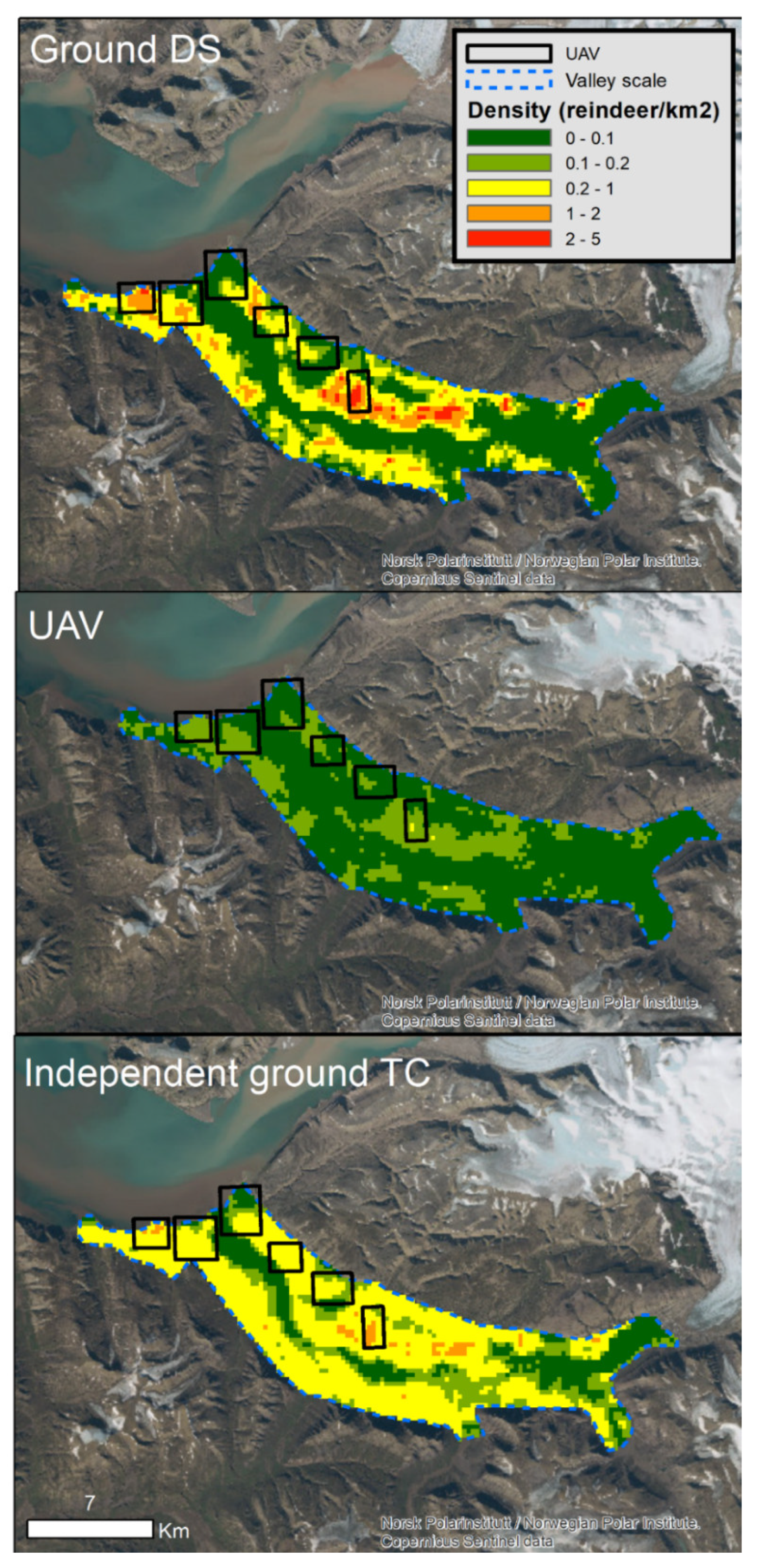
To assess each survey method, we chose to predict each density model across: (1) The ground DS covered area, (2) the UAV covered area, and (3) at an ecologically relevant valley scale for management. Since the habitat characteristics and elevation ranges were different for the helicopter surveyed area (0.6–601 m) than for the ground and UAV transect area (0.7–317 m), we did not predict the ground DS and UAV density models to the helicopter surveyed area. Estimates were compared to the the ground DS and precisions were compared with the coefficient of variation (CV, the ratio of the standard deviation to the mean). Lower CV indicates higher precision.

3. Results

3.1. Field Survey Characteristics

The ground DS survey detected 50 groups of reindeer (n = 104 individuals, mean group size = 2), walking 23.6 km on foot with a transect truncation width of 907 m (i.e., covering an area of 42.7 km2). The UAV survey, which covered about 40% of the same transects (16.2 km2), detected 32 confirmed reindeer. The helicopter survey covered the largest area (286.2 km2) and resulted in 1559 observed reindeer (Figure 1). The range in vegetation productivity within the three sampling areas were similar (range for ground DS [0.04–0.82], UAV [0.09–0.82] and helicopter [0.04–0.82]), with a mean maxNDVI of approximately 0.50.

3.2. Detection of Reindeer

The average detection probability for the ground DS survey was 0.40 ± 0.10 with 30% of the reindeer clusters detected within approximately 500 m. Sunny weather conditions resulted in higher reindeer detectability than cloudy (Figure A2). For the UAV survey, the average detection rate of confirmed reindeer varied between observers by 46–70% (n = 6). Variation of reindeer detection in the UAV imagery for the presence/absence model showed an association with the greenness index and blue color channels when accounting for observer variability (Figure 3). High values in the greenness index (i.e., greener vegetation ground cover) resulted in increased detectability, while high values of the blue channel decreased detectability. In addition, all variables associated with darker ground, except for the greenness index, decreased the probability to count the correct number of reindeer in an image when at least one reindeer was present (Figure A7, Table A5).

3.3. Reindeer Densities and Spatial Projections

All three DSMs predicted a positive correlation between vegetation productivity (maxNDVI) and reindeer densities (Figure 4). Reindeer density remained low until around maxNDVI of 0.6–0.7 and thereafter increased steeply. However, the strength of the relationship was markedly lower for UAV, while the ground DS and independent total counts were similar (Figure 4).
The independent total counts model from the neighboring valley estimated similar abundances in the helicopter surveyed area (1515 ± 101, Table 1) as the helicopter survey (n = 1559) in Sassendalen. The UAV density model estimated the lowest abundances with the largest uncertainties (i.e., CVs range: 0.11–0.29), underestimating abundance by 70–75% compared to ground DS and UAV at the different sampling scales. The ground DS and the independent ground TC estimated similar abundance at all sampling scales. The independent ground TC gave the most precise estimates (CVs range: 0.07–0.24), while ground DS precision was intermediate (CVs range: 0.22–0.26) (Table 1, Figure 5).

4. Discussion

Our comparison of the different survey methods—ground DS, UAV, helicopter, and independent ground TC surveys—for estimating Svalbard reindeer abundance and density showed that UAV imagery underestimated the number of reindeer as compared to all three other methods. It was feasible to identify reindeer, calculate precision and investigate factors affecting observers’ detection of reindeer using UAV, however, the UAV count was not able to capture accurate density patterns compared to the other survey methods. We therefore address key challenges to improve count accuracy of UAV at a meaningful scale for species management.
Wildlife surveys with a coefficient of variation (CV) of less than 0.25 is often considered useful for research and wildlife management [53]. In our study, ground DS, UAV and independent ground TC surveys all had a CV of less than 0.25 at the valley scale, which means that all three survey methods can detect smaller changes in reindeer abundances at a management-relevant scale. Although the UAV survey had the highest CV in our study (0.29), the median precision of estimates in other ungulate surveys is around 0.42, and only 26.4% of the abundance estimates reported a CV below 0.25 [3]. This means that the precision of estimates from the UAV survey resembles other ungulate studies in the field but is not as accurate as the traditional ground survey methods used previously to estimate reindeer abundance in Svalbard.
Precise but biased counts have little value for informing management. Biased estimation of abundance can result from a variety of sources, including violation of statistical assumptions, survey design or observer variability [3]. Here, the UAV survey underestimated abundances compared to the reference ground DS, previously demonstrated as an accurate methodology [20,22]. Although the area covered by the quadcopter (16.2 km2) is on the higher end of what other studies counting animals with UAV have reported [7], it was challenging to obtain a large enough sample size in relation to the UAV covered area. Few reindeer were present in the UAV area covered, despite the high density and detectability of Svalbard reindeer found at the valley scale (5.7 reindeer/km2 from the reference ground DS). Doing repeat surveys over the same transect lines would increase precision by increasing sample size, as recommended for low-density animals [54], but still lead to biased estimates if the area is too small to capture densities in various habitat characteristics [54]. For this wide-ranging species, unbiased estimates require large enough areas to capture the density gradients across the range of habitat.
Observer variability is due to non-detection of individuals that are present (false negatives) or misidentification of individuals (false positives) [15]. In our study, we minimised these forms of detection error by having multiple observers scanning the same UAV imagery and later manually reviewing the detected reindeer to remove misidentified individuals [55]. Images with high values of the greenness index (G-B [51]) increased the likelihood of reindeer detection, likely reflecting that dark reindeer are more distinguishable from the green, vegetated background. Images with high mean blue values decreased reindeer detection, and blue as a dominant reflection can be due to, e.g., gravel, rock, or barren ground, which will make the brownish fur of reindeer blend better in and be more difficult to detect. Observers in aerial surveys are prone to underestimate animal abundances, especially group size [15], and integrating forms of detection probability in future model development of animal density functions for drone imagery will improve accuracy. For instance, the strip transect framework by Buckland et al. [20], modelled with a uniform key detection function (in ‘ds’ in the Distance package), or both model parts of a hurdle model (i.e., presence/absence and count model in ‘hurdle’ in the pscl package), currently assumes perfect detection. This is rarely the case in practice. Development of these R-functions, allowing for imperfect detection and inclusion of covariates driving detection is beneficial to UAV studies, as UAV survey techniques are rapidly increasing in wildlife studies.
Here, we conducted the UAV survey in an open tundra landscape with good visibility from the air (at 120 m) and with no terrain obstacles hindering the drone. This flying height permitted the maximum area to be covered at which a reindeer could be detected with minimal disturbance. Retrospectively, we could have increased detection of animals by flying at lower heights (i.e., the observers would have been less uncertain about distinguishing an animal from a background feature) and thus reduced observer variability further. This comes at the cost of longer flight times due to lower swath width (i.e., denser mapping flight lines) and thus even smaller covered areas and more imagery to scan. A way to compensate for the increased flight time is to reduce the side or forward overlap to a lower value. In such cases, the overlap can be reduced below 50%, thereby decreasing the amount of flying time. Before implementing such adjustments, the effect of UAV disturbance on reindeer should be carefully assessed in a separate study.
Studies that report aerial surveys being more accurate than traditional survey methods often have issues with detectability in the traditional survey methods. This is the case with counting rare deer in dense forests, where ground counts are ineffective due to forest cover and low densities of deer [8], where aerial imagery may provide better overview or spatial coverage. This may also be the case when there are challenges detecting marine animals at the sea surface from boats [9,10,25]. In our study, the ground DS survey had a maximum line of sight of about 900 m, three times more compared to other study systems with lower linear detection rates, such as DS conducted on deer in woody, heterogenous terrain (250 m; [56]). By comparing the helicopter count with the independent ground TC, a methodology previously investigated as highly accurate and which here match the ground DS estimates [21,22], we were able to assess that this helicopter count was unbiased. Thus, using the relation from reindeer density to vegetation productivity from a neighbouring valley, we were able to capture the spatial density in the focal study system [32], as expected from the documented spatial synchrony in population dynamics from this region. A measure of precision is crucially needed also for the helicopter survey and recording reindeer geographic positions and assessing detection probability will greatly improve the survey design.
To address the challenge of limited area and line of sight covered by our small quadcopter drone, we suggest testing a UAV with longer range to increase the area covered and types of tundra habitats with different textures and densities of reindeer. The UAV used in this pilot study had limited battery capacity and flying time. Using larger quadcopter drones or fixed-wing drones with a longer range allows for covering larger areas where abundance can be estimated [37,57]. This, however, comes at higher costs and in the case of fixed-wing drones, higher operation complexity, particularly in remote Arctic regions. Therefore, it was a sensible approach to first verify the methodology with a small quadcopter, as in this pilot study. Once the method is fully developed and evaluated it can be easily transferred to more complex UAV systems that compensate for the limited range and coverage (i.e., using fixed-wing UAVs) [37].
The large number of images that our UAV survey produced exemplifies key challenges of any aerial survey methods, namely counting the animals in the images. To increase the efficiency of the process, orthomosaics were generated and tiled into “easy-to-handle” single images. This reduced the number of images to scan and made the process more efficient. In the stitching process, reindeer may disappear or appear multiple times. By scanning and comparing the raw imagery with the tiled imagery after the stitching process, we quantified this disappearance, but at the expense of much longer processing time. In the case of the disappearing reindeer, the reindeer were moving over heterogenous terrain (e.g., from riverbed into swampy wetland areas). This large gradient in surface texture of the different habitat types may explain why the algorithm resulted in removing the reindeer in the stitching process. However, reindeer that remained stationary, or moved over homogenous terrain did not appear multiple times, nor did they disappear in the orthomosaic process. Datasets from UAV surveys with low-density populations in open landscapes seem particularly well-suited for automated counting methods, e.g., using machine learning [58]. However, this requires large training data sets of reindeer in a varity of habitat types with different surface texture and there is a need to make manual counts more efficient [58]. We encourage future studies to focus on developing training datasets using the protocol we have presented (Appendix C) as a key towards automated detection methods.

5. Conclusions

Reliable estimates of wildlife population abundance provide information, which is necessary to make conservation and management decisions. With this pilot study, we confirmed that it is possible to identify, count, collect geographical positions, and quantify covariates affecting detection of reindeer on UAV imagery. UAVs have the potential to be an alternative to traditional monitoring methods for estimating Svalbard reindeer abundance, if key aspects are improved: (1) Increase the covered area to capture the density-vegetation productivity gradient of this wide-ranging species, (2) integrate imperfect detection in hurdle models, and (3) reduce imagery processing time. While the results gathered in this study with a quadcopter UAV are limited in their value—due to the underestimation of reindeer abundance and the data acquisition time—they serve as a proof of concept. The limitations can be overcome by utilizing UAV platforms that cover larger areas in shorter time and conducting repeat surveys over the same transects. This can be achieved, for example, by using fixed-wing UAVs with substantially larger range and endurance compared to multirotor drones. With larger datasets, more individual reindeer will be sampled. This is likely to increase the possibility to use machine learning algorithms to automate the counting process. The relative lower carbon footprint and lesser human disturbance compared to helicopter surveys encourage further UAV method development in remote Arctic regions. Before limitations are addressed, UAV surveys may be a supplement to the traditional, ground-based field methods but cannot yet fully replace them when it comes to herbivore monitoring in open heterogenous landscapes. Our study demonstrates the importance of a thorough quality assessment of survey methods before results are applied for management inference.

Author Contributions

Å.Ø.P. and I.M.G.P. have contributed equally the article. Conceptualisation, Å.Ø.P., I.M.G.P., M.L.M., I.E., A.S. and V.T.R.; methodology, M.L.M., I.M.G.P., M.-A.B., Å.Ø.P. and R.H.; software, R.H. and I.M.G.P.; formal analysis, I.M.G.P., M.L.M., M.-A.B. and R.H.; investigation, R.H., M.L.M., I.M.G.P., Å.Ø.P. and C.v.H.; resources (equipment, environmental data, etc.), R.H., I.M.G.P., Å.Ø.P., V.T.R.; writing—original draft preparation, Å.Ø.P., I.M.G.P., M.L.M. and R.H.; writing—review and editing, all authors; visualisation, I.M.G.P. and M.L.M.; supervision, M.L.M. and Å.Ø.P.; project administration, Å.Ø.P.; funding acquisition, Å.Ø.P., I.M.G.P., M.L.M., A.S. and V.T.R. All authors have read and agreed to the published version of the manuscript.

Funding

This research was funded by Svalbard Environmental Protection Fund (19/120), Svalbard Integrated Arctic Earth Observing System, the Norwegian Polar Institute, Norwegian University of Science and Technology and (Norwegian Research Council FRIPRO 276080 and SFF-III 223257).

Data Availability Statement

Hann, R. 2022. Drone-based mapping of Sassendalen for reindeer counting in Svalbard. DataverseNO. V1. Doi: 10.18710/KHQKWH. Pedersen, Å. Ø. (2022). Svalbard reindeer distance sampling dataset in Sassendalen 2021. Norwegian Polar Institute. https://doi.org/10.21334/npolar.2022.8f2c11ff (accessed on 9 October 2022).

Acknowledgments

We thank Jørn Dybdahl for excellent support during the field work, Oddveig Øien Ørvoll and Bernt Bye for cartographic assistance, and the Governor of Svalbard for use of the Fredheim cabin. We also thank the people that counted the reindeer imagery David Studer, Anna Caroline Grimsby, Beate Garfelt, and Stein Tore Pedersen. Stein Rune Karlsen for providing NDVI-maps and Gunn Sissel Jaklin for proofreading the manuscript.

Conflicts of Interest

The authors declare no conflict of interest.

Appendix A. Independent Total Counts from Adventdalen—Background Data and Results

Statistical Analyses

The values of all average maxNDVI pixels (240 × 240 m) in the sampling area (Adventdalen below 250 m) were extracted (n = 3262 pixels), including all pixels with at least one geographic position of a reindeer observation (n = 437 pixels, min positions per pixel = 1, max positions per pixel = 22). There was positional information for 1527 out of 1668 reindeer groups. Mean reindeer group size was 3.2 reindeer. The hurdle model was applied to this dataset with maxNDVI as a covariate and observations per pixel as a response variable. The best model was determined by AIC. Based on results from the best model from the total counts in Adventdalen, a density map was created across the Sassendalen valley in the same area as the helicopter surveyed area.
Figure A1. Reindeer geographic positions in the Sassendalen’s neighboring valley Adventdalen (n = 1527).
Remotesensing 15 00009 g0a1
Table A1. Independent total counts density model obtained from ground counts in a neighboring valley. We used the most parsimonious density model for total counts from Le Moullec et al. [22], which modelled individuals per segment as a function of maxNDVI using a hurdle density model with a zero-truncated negative binomial distribution with a dispersion parameter. This model was fitted using the restricted maximum likelihood (REML) framework. The model presented below is the model with the highest AIC.
Hurdle Density Model Adventdalen
β ± SEp
Count modelIntercept−1.04 ± 0.570.07
NDVI *0.003 ± 0.00090.002
P/A modelIntercept−4.59 ± 0.33<0.05
NDVI *0.004 ± 0.00050.02
* NDVI is the average maximum NDVI from 2017–2021.

Appendix B. Model Selection and Detection Curve for Estimating Svalbard Reindeer Abundance by Ground Distance Sampling

Table A2. The four candidate detection probability models for Distance sampling (DS) of Svalbard reindeer, Svalbard, Norway (July 2021). Detection probability was fitted using half-normal (hn) and hazard rate (hr) functions with weather (sunny or cloudy) as covariate (see Table S3 in Le Moullec et al. [22] for the influence of other covariates). We ranked models using Akaike’s Information Criterion (AIC) and differences in AIC (ΔAIC).
ModelKeyAICΔAIC
~weatherhr657.8930
~1hr661.4773.584
~weatherhn663.6275.734
~1hn665.8577.964
Figure A2. Detection probability function based on the line transect distance sampling of Svalbard reindeer. The best model was fitted at a continuous scale for observed distances and included a hazard rate key detection function with weather (sunny or cloudy) as covariate. Observations of reindeer clusters are illustrated by dots along the curve.
Remotesensing 15 00009 g0a2
Table A3. Density model obtained from ground distance sampling. We used the most parsimonious density model from Le Moullec et al. [22], which modelled individuals per segment as a function of NDVI using a log-link quasi-Poisson model. This model was fitted using the restricted maximum likelihood (REML) framework.
Ground DS Survey SassendalenModel by Le Moullec et al. [22]
β ± SEpβ ± SEp
Intercept−19.25 ± 2.05<0.001−13.95 ± 0.38<0.001
NDVI *0.012 ± 0.003<0.0012.65 × 10−3 ± 0.76 × 10⁻³<0.001
* Le Moullec et al., 2019 is based on average maxNDVI from 2013–2016.
Figure A3. Density function modelling individuals per segment as a function of NDVI using a log-link quasi-Poisson model. The model was fitted using the restricted maximum likelihood (REML). Displayed above are diagnostic plots for the selected model using the function ‘gam.check’ in the package mgcv.
Remotesensing 15 00009 g0a3

Appendix C. Protocol for Counting Reindeer from UAV Imagery

Appendix C.1. Counting Svalbard Reindeer from Drone Imagery—Instructions to Observers (Full Version Can Be Available from the Authors upon Request)

Background

In this protocol you will count Svalbard reindeer in UAV imageries captured in Sassendalen, Svalbard in July 2021. Six predefined transects were flown with a multirotor at an altitude of 100–120 m over reindeer habitats. The images were merged and postprocessed into evenly sized tiles by Richard Hann (NTNU). The objective for you as an observer is to help identify reindeer from the UAV imagery and assign them into simple sex and age categories, so they can be compared with helicopter and ground surveys done the same year.
The software you will use to count the reindeer is called DotDotGoose ver. 1.5.1 [59]. DotDotGoose is a free, open-source tool to assist with counting objects manually in images. The software was created by the American Museum of Natural History to assist conservation researchers and practitioners working on counting objects in any kind of image format. The benefit of DotDotGoose is that you can easily create custom classes, pan and zoom on images and place points to identify individual objects. The metadata from each observer will be exported for further analyses in this project.
The reindeer categories you will identify in the UAV images correspond to sex and age classes used in helicopter counts (Governor of Svalbard 2009) and ground surveys ([total counts; 21]). These are (1) reindeer with large antlers (old male), (2) reindeer with small antlers (female/young), (3) reindeer without antlers (female/young), (4) calves, (5) reindeer you are unsure in which category they belong, and (6) carcasses. Carcasses are not counted in helicopter surveys but come in addition because it will help you to keep focused since there are many images without reindeer in them.
The categories may look like the photos below on the UAV imagery (Figure A4 and Figure A5). Note that key characteristics of a reindeer is the body shape, the color (white and grey) and sometimes the shadow. The shadow can sometimes help to determine the size of the antlers (if antlers are present). Be aware that the objects are pixelated and blurry and it may not always be easy to distinguish the objects, especially if the reindeer are lying down.
Figure A4. Overview of the five classes to categorise reindeer from drone imagery.
Remotesensing 15 00009 g0a4aRemotesensing 15 00009 g0a4b
Figure A5. A full-scale image like the one you will see when you go through the images and classify reindeer into one of the five categories in Figure A7. Do you see a reindeer? Try to remember the size of the reindeer relative to the full-scale image. If you see anything that resembles a reindeer, you can zoom in using the buttons on the left.
Remotesensing 15 00009 g0a5
For more information about the software (other than what is in this protocol) check out the DotDotGoose QuickGuide in the folder or this video tutorial on how to use the software: https://www.youtube.com/watch?v=VGxTiQHx4Lc (accessed on 7 December 2020).

Appendix C.2. Download Software and Get Started!

Save and extract the ‘Reindeer_counting_drone_imagery.zip’ to your computer or hard disk. The folder and metadata require about 4 GB of space so make sure you have enough.

Appendix C.3. Set up DotDotGoose Software

Click and open the dotdotgoose.exe file in the ‘Reindeer_counting_drone_imagery’ folder
Click on ‘Load’ in the bottom left corner. Find the imagery folder “drone_imagery_SAS_2021” and select the point file ‘template_reindeer_counting.pnt’
In Survey Id at the top left panel: put your first name and last name with underscore, e.g., ole_olesen. This will create a column in the metadata with your name.
Click the Save button and save a point file with your own name (e.g., ole_olesen.pnt) into the same folder as the drone imagery ‘drone_imagery_SAS_2021’. It is important that it is the same folder as the imagery—if not the save will not work!
If you need to close the programme and finish at another time, you can open your point file in the DotDotGoose software by locating the file and click Import.

Appendix C.4. Reindeer Detection and Assigning Objects to Categories

Appendix C.4.1. Time Tracking

We would like to know how long it takes for each observer to scan through each transect line. The name of each jpeg file starts with the transect number (e.g., Line_1, Line_2).
When you are about to start on the first image of the transect (e.g., Line_1_tile_100.jpeg) write down the time in ‘time_start’ from the Custom Fields (right side panel) from your computer clock (e.g., 09:54).
When you have scanned all images in the transect (e.g., last image is Line_1_tile_99.jpeg) write down the time in time_stop (e.g., 11:00) on this last image of Line_1.
Do this for every transect line (Line_1 to Line_6) so we get the start and end time for each transect. Please try to complete every transect line in one go, but if you need to take breaks write down the end time and start time as well so breaks can be subtracted.
Remember to save frequently and when you take breaks.

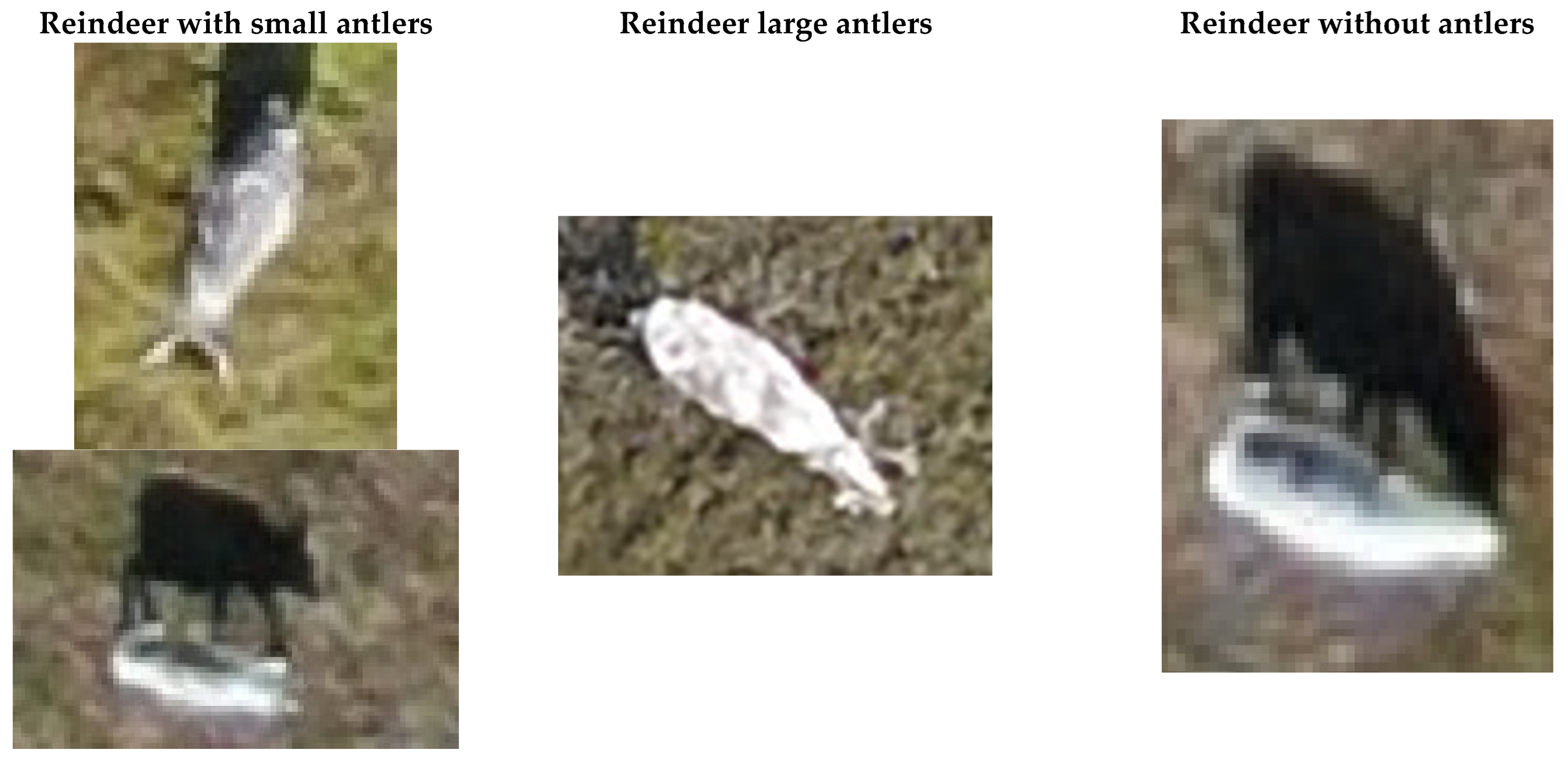
Appendix C.4.2. Reindeer Scanning Method

For each image, scan the full-scale image quickly from grid to grid with your eyes (see example below). It might be useful to move your mouse as a guide.
If you cannot find an object of interest, go to the next image by pressing the down arrow key on your keyboard.
If you want to go back to any previous images use the up-arrow key or double-click on a specific photo in the Summary table.
Figure A6. Example of how to scan an image.
Remotesensing 15 00009 g0a6
If you do find an object of interest, zoom in on it to check if it is a reindeer or carcass by scrolling your mouse or use the zoom buttons in the right bottom corner (you can also drag the image up, down, and sideways by clicking and holding the mouse).
To mark a reindeer or carcass, you click on the category you want to assign on the left side panel (see left image below). Press the Ctrl key while you click on the object in the image. A dot will be created over the reindeer.
You can double check that the right category was assigned to the object for that image by looking at the Summary table on the left panel (see right image below).
NB! If you accidentally make a point or assign wrong category and need to remove it from the image, press and hold the Shift key on your keyboard, then left click and drag the mouse to draw a box around the points you’d like to delete. A red circle around your point will show up. Press the Delete key to remove the point.

Appendix D. UAV Density Model for Estimating Reindeer Abundance with Hurdle Density Model

Table A4. UAV density model obtained from UAV sampling in Sassendalen in 2021. We used the most parsimonious density model from Le Moullec et al. [22], which modelled individuals per segment as a function of NDVI using a Hurdle density model with a zero-truncated negative binomial distribution with a dispersion parameter. Displayed below are the two candidate models with lowest AIC. Both models were fitted using the restricted maximum likelihood (REML). The simplest of the two models, Hurdle model 2, was selected for the analyses.
UAV Density Models
β ± SEpAICΔAIC
Hurdle 1Count modelIntercept−2.61 ± 82.80.975182.500
NDVI−9.59 ± 7.150.180
P/A modelIntercept−7.00 ± 1.40<0.05
NDVI6.67 ± 2.150.002
Hurdle 2Count modelIntercept114.19 ± −0.080.93182.540.04
Log(theta)−10.16 ± 114.200.93
P/A modelIntercept−5.82 ± 1.36<0.05
NDVI5.19 ± 2.0800.012

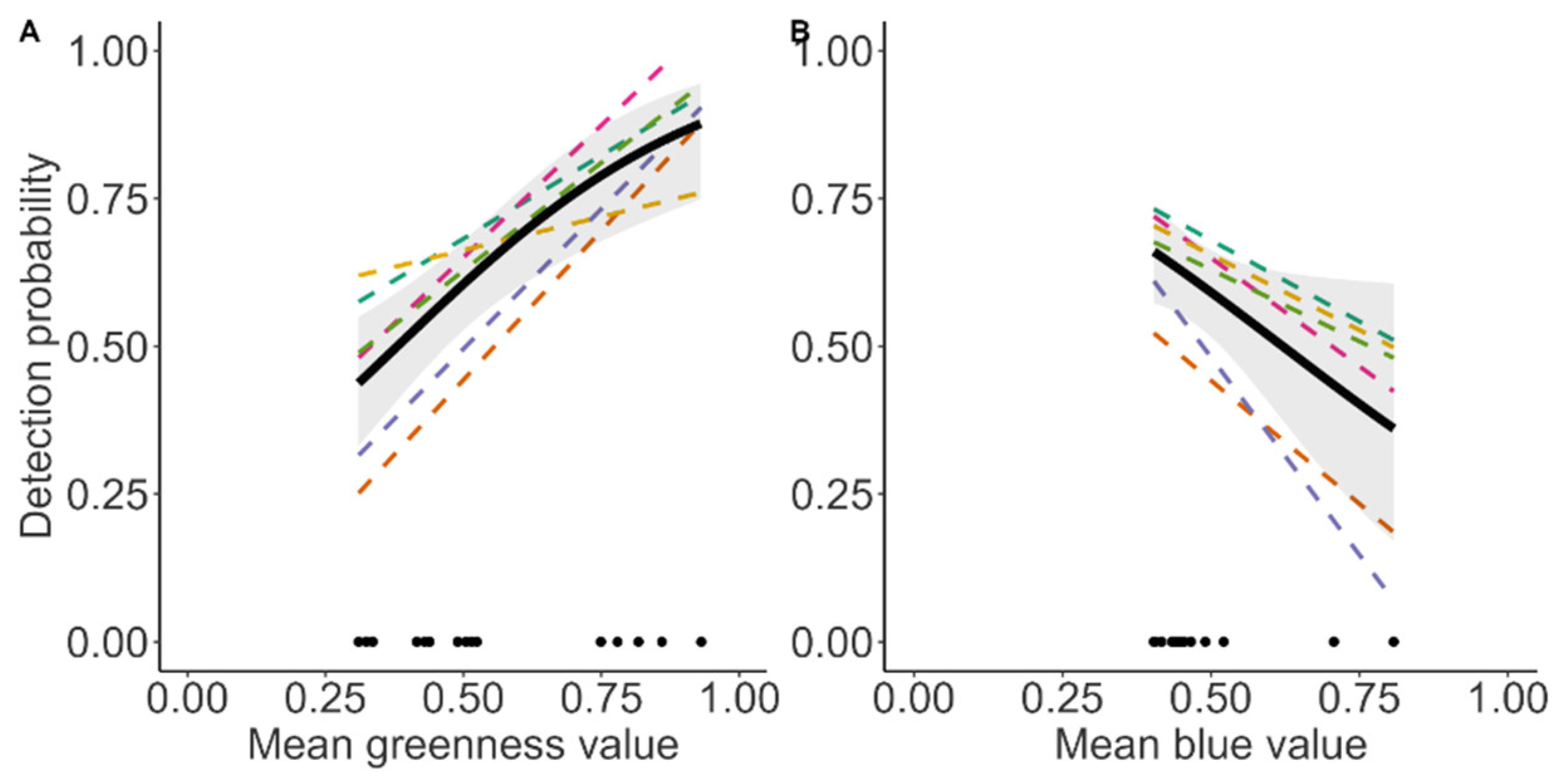
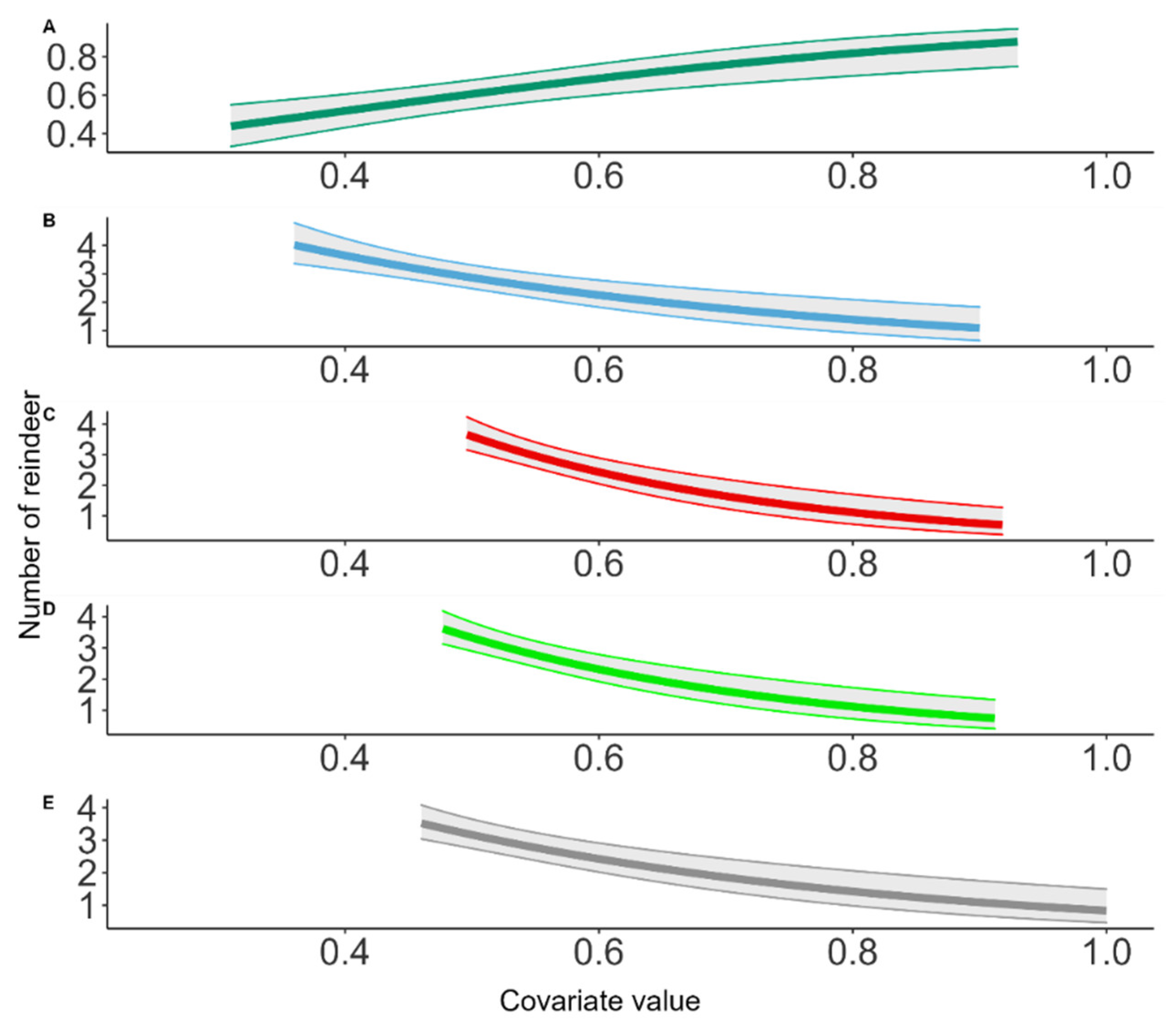
Appendix E. Detection Probability from UAV Imagery

The linear mixed effects models (glmer function), implemented in the lme4 package in R, were developed based on two sources of detection errors related to the probability that (1) an observer detects a reindeer in an image (presence/absence model) and (2) when they do, how many reindeer are detected in that image (counts model). The reason for this was also to develop detection models to fit the two-function process in the density model. For the presence/absence model, all reindeer detected by observers (verified as a reindeer (1) or not (0)) were given an ID based on their GPS coordinates. The image covariates median luminance, mean red, mean green, and mean blue channels were extracted from each image using the package imageR. High values in the red and blue channel indicated grey, gravely backgrounds. The RGB greenness index (G-B, [51]) was calculated to identify green background (low values = dark green, high values = light green). Due to multicollinearity in covariates, we ran separate models including each of the individual covariate as fixed effect and observer ID as a random effect.
Presence/absence model
  • Binomial linear mixed effect model (GLMER)
  • Five separate models with observer id as a random effect and each of the fixed effects median luminance, mean red, green, and blue channels per image. We only show the predicted effect plots for the fixed effects with a statistical significance (p > 0.05) below (intercepts and standard error in results section).
  • Response variable: Reindeer seen (1) or reindeer not seen (0) by observers
  • Sample size of reindeer n = 234
Count model
  • Poisson GLMER.
  • Five models with observer id as a random effect and each of the fixed effects median luminance, mean red, green, and blue channels per image (intercepts and standard error in results section). Below, we only show the predicted effect plots for the fixed effects with a statistical significance (p > 0.05)
  • Response variable: Number of reindeer observed in an image
  • Sample size of reindeer n = 179
Figure A7. Predicted effects of each covariate in the five separate GLMER counts model. (A) greenness index, (B) mean blue channel, (C) mean red channel, (D) mean green channel, (E) median luminance.
Remotesensing 15 00009 g0a7
Table A5. Model estimates from the ten separate GLMERs for UAV P/A (n = 234, 6 observers) and UAV count model (n = 179, 6 observers). The coefficients are on a logit scale for the P/A models and Poisson scale for the count models. Bold denotes significant covariate effects (p < 0.05). Random effect is reported as variance and standard deviation.
Fixed EffectRandom EffectCoefficientFixed Effect
(Β ± Se)
Random EffectAIC
P/A model~Greenness indexobserver IDIntercept
Covariate
−1.36 ± 0.48
3.57 ± 0.92
0.04, 0.20301.89
~mean blue channelobserver IDIntercept
Covariate
1.90 ± 0.73
−3.06 ± 1.48
0.03, 0.17315.10
~mean green channelobserver IDIntercept
Covariate
1.63 ± 0.85
−2.25 ± 1.58
0.03, 0.17317.43
~mean red channelobserver IDIntercept
Covariate
1.35 ± 0.89
−1.67 ± 1.61
0.03, 0.16318.40
~median luminanceobserver IDIntercept
Covariate
1.07 ± 0.68
−1.22 ± 1.28
0.03, 0.16318.57
Count model~mean red channelobserver IDIntercept
Covariate
−3.91 ± 0.76
−3.91 ± 0.76
0.02, 0.13709.63
~mean green channelobserver IDIntercept
Covariate
3.01 ± 0.38
−3.62 ± 0.72
0.02, 0.13712.19
~median luminanceobserver IDIntercept
Covariate
−2.66 ± 0.57
−2.66 ± 0.57
0.02, 0.14714.17
~mean blue channelobserver IDIntercept
Covariate
−2.41 ± 0.58
−2.41 ± 0.58
0.02, 0.13725.01
~Greenness indexobserver IDIntercept
covariate
1.40 ± 0.14
−0.52 ± 0.22
0.03, 0.18740.84

References

  1. Nichols, J.D.; Williams, B.K. Monitoring for conservation. Trends Ecol. Evol. 2006, 21, 668–673. [Google Scholar] [CrossRef] [PubMed]
  2. Williams, B.K.; Nichols, J.D.; Conory, M.J. Analysis and Management of Wildlife Populations; Academic Press: San Diego, CA, USA, 2002. [Google Scholar]
  3. Forsyth, D.M.; Comte, S.; Davis, N.E.; Bengsen, A.J.; Cote, S.D.; Hewitt, D.G.; Morellet, N.; Mysterud, A. Methodology matters when estimating deer abundance: A global systematic review and recommendations for improvements. J. Wildl. Manag. 2022, 86, e22207. [Google Scholar] [CrossRef]
  4. Thompson, W.L.; White, G.C.; Gowan, C. Chapter 3—Enumeration Methods. In Monitoring Vertebrate Populations; Thompson, W.L., White, G.C., Gowan, C., Eds.; Academic Press: San Diego, CA, USA, 1998; pp. 75–121. [Google Scholar]
  5. Gamelon, M.; Firth, J.A.; le Moullec, M.; Petry, W.K.; Salguero-Gòmez, R. Longitudinal demographic data collection. In Demographic Methods Across the Tree of Life; Roberto Salguero-Gomez, M.G., Ed.; Oxford Academic: Oxford, UK, 2021. [Google Scholar]
  6. ENETWILD consortium; Grignolio, S.; Apollonio, M.; Brivio, F.; Vicente, J.; Acevedo, P.; Palencia, P.; Petrovic, K.; Keuling, O. Guidance on estimation of abundance and density data of wild ruminant population: Methods, challenges, possibilities. EFSA Support. Publ. 2020, 17, 1876E. [Google Scholar] [CrossRef]
  7. Wang, D.L.; Shao, Q.Q.; Yue, H.Y. Surveying Wild Animals from Satellites, Manned Aircraft and Unmanned Aerial Systems (UASs): A Review. Remote Sens. 2019, 11, 1308. [Google Scholar] [CrossRef] [Green Version]
  8. Pereira, J.A.; Varela, D.; Scarpa, L.J.; Frutos, A.E.; Fracassi, N.G.; Lartigau, B.V.; Pina, C.I. Unmanned aerial vehicle surveys reveal unexpectedly high density of a threatened deer in a plantation forestry landscape. Oryx 2022, First View, 1–9. [Google Scholar] [CrossRef]
  9. Schofield, G.; Esteban, N.; Katselidis, K.A.; Hays, G.C. Drones for research on sea turtles and other marine vertebrates—A review. Biol. Conserv. 2019, 238, 108214. [Google Scholar] [CrossRef]
  10. Fettermann, T.; Fiori, L.; Gillman, L.; Stockin, K.A.; Bollard, B. Drone surveys are more accurate than boat-based surveys of bottlenose dolphins (Tursiops truncatus). Drones 2022, 6, 82. [Google Scholar] [CrossRef]
  11. Hodgson, J.C.; Mott, R.; Baylis, S.M.; Pham, T.T.; Wotherspoon, S.; Kilpatrick, A.D.; Raja Segaran, R.; Reid, I.; Terauds, A.; Koh, L.P. Drones count wildlife more accurately and precisely than humans. Methods Ecol. Evol. 2018, 9, 1160–1167. [Google Scholar] [CrossRef] [Green Version]
  12. Forsyth, D.M.; MacKenzie, D.I.; Wright, E.F. Monitoring ungulates in steep non-forest habitat: A comparison of faecal pellet and helicopter counts. N. Z. J. Zool. 2014, 41, 248–262. [Google Scholar] [CrossRef]
  13. Noyes, J.H.; Johnson, B.K.; Riggs, R.A.; Schlegel, M.W.; Coggins, V.L. Assessing aerial survey methods to estimate elk populations: A case study. Wildl. Soc. Bull. 2000, 28, 636–642. [Google Scholar]
  14. Poole, K.G.; Cuyler, C.; Nymand, J. Evaluation of caribou Rangifer tarandus groenlandicus survey methodology in West Greenland. Wildl. Biol. 2013, 19, 225–239. [Google Scholar] [CrossRef]
  15. Davis, K.L.; Silverman, E.D.; Sussman, A.L.; Wilson, R.R.; Zipkin, E.F. Errors in aerial survey count data: Identifying pitfalls and solutions. Ecol. Evol. 2022, 12, e8733. [Google Scholar] [CrossRef] [PubMed]
  16. Reilly, B.K.; van Hensbergen, H.J.; Eiselen, R.J.; Fleming, P.J.S. Statistical power of replicated helicopter surveys in southern African conservation areas. Afr. J. Ecol. 2017, 55, 198–210. [Google Scholar] [CrossRef]
  17. Dyal, J.; Miller, K.V.; Cherry, M.J.; D’Angelo, G.J. Estimating sightability for helicopter surveys using surrogates of white-tailed deer. J. Wildl. Manag. 2021, 85, 887–896. [Google Scholar] [CrossRef]
  18. Mansson, J.; Hauser, C.E.; Andren, H.; Possingham, H.P. Survey method choice for wildlife management: The case of moose Alces alces in Sweden. Wildl. Biol. 2011, 17, 176–190. [Google Scholar] [CrossRef] [Green Version]
  19. Gentle, M.; Finch, N.; Speed, J.; Pople, A. A comparison of unmanned aerial vehicles (drones) and manned helicopters for monitoring macropod populations. J. Wildl. Res. 2018, 45, 586–594. [Google Scholar] [CrossRef]
  20. Buckland, S.T.; Anderson, D.R.; Burnham, K.P.; Laake, J.L.; Borchers, D.L.; Thomas, L. Introduction to Distance Sampling: Estimating Abundance of Biological Populations; Oxford University Press: Oxford, UK, 2001; pp. 1–432. [Google Scholar]
  21. Le Moullec, M.; Pedersen, A.O.; Yoccoz, N.G.; Aanes, R.; Tufto, J.; Hansen, B.B. Ungulate population monitoring in an open tundra landscape: Distance sampling versus total counts. Wildl. Biol. 2017, 2017, 1–11. [Google Scholar] [CrossRef] [Green Version]
  22. Le Moullec, M.; Pedersen, Å.Ø.; Stien, A.; Rosvold, J.; Hansen, B.B. A century of conservation: The ongoing recovery of svalbard reindeer. J. Wildl. Manag. 2019, 83, 1676–1686. [Google Scholar] [CrossRef]
  23. Delplanque, A.; Foucher, S.; Lejeune, P.; Linchant, J.; Théau, J. Multispecies detection and identification of African mammals in aerial imagery using convolutional neural networks. Remote Sens. Ecol. Conserv. 2022, 8, 166–179. [Google Scholar] [CrossRef]
  24. Yang, F.; Shao, Q.; Jiang, Z. A population census of large herbivores based on UAV and its effects on grazing pressure in the Yellow-River-Source National Park, China. Int. J. Environ. Res. Public Health 2019, 16, 4402. [Google Scholar] [CrossRef] [Green Version]
  25. Butcher, P.A.; Colefax, A.P.; Gorkin, R.A.; Kajiura, S.M.; López, N.A.; Mourier, J.; Purcell, C.R.; Skomal, G.B.; Tucker, J.P.; Walsh, A.J.; et al. The drone revolution of shark science: A review. Drones 2021, 5, 8. [Google Scholar] [CrossRef]
  26. Descamps, S.; Aars, J.; Fuglei, E.; Kovacs, K.M.; Lydersen, C.; Pavlova, O.; Pedersen, A.O.; Ravolainen, V.; Strom, H. Climate change impacts on wildlife in a High Arctic archipelago—Svalbard, Norway. Glob. Chang. Biol. 2017, 23, 490–502. [Google Scholar] [CrossRef]
  27. van der Wal, R.; Bardgett, R.D.; Harrison, K.A.; Stien, A. Vertebrate herbivores and ecosystem control: Cascading effects of faeces on tundra ecosystems. Ecography 2004, 27, 242–252. [Google Scholar] [CrossRef]
  28. Peeters, B.; Pedersen, Å.Ø.; Veiberg, V.; Hansen, B.B. Hunting quotas, selectivity and stochastic population dynamics challenge the management of wild reindeer. Clim. Res. 2022, 86, 93–111. [Google Scholar] [CrossRef]
  29. Hansen, B.B.; Gamelon, M.; Albon, S.D.; Lee, A.M.; Stien, A.; Irvine, R.J.; Saether, B.E.; Loe, L.E.; Ropstad, E.; Veiberg, V.; et al. More frequent extreme climate events stabilize reindeer population dynamics. Nat. Commun. 2019, 10, 1–8. [Google Scholar] [CrossRef] [Green Version]
  30. Loe, L.E.; Liston, G.E.; Pigeon, G.; Barker, K.; Horvitz, N.; Stien, A.; Forchhammer, M.; Getz, W.M.; Irvine, R.J.; Lee, A.; et al. The neglected season: Warmer autumns counteract harsher winters and promote population growth in Arctic reindeer. Glob. Chang. Biol. 2021, 27, 993–1002. [Google Scholar] [CrossRef]
  31. Solberg, E.J.; STrand, O.; Veiberg, V.; Andersen, R.; Heim, M.; Rolandsen, C.M.; Langvatn, R.; Holmstrøm, F.; Solem, M.I.; Eriksen, R.; et al. Hjortevilt 1991–2011. Oppsummeringsrapport fra Overvåkingsprogrammet for hjortevilt. NINA Rapp. 2012, 885, 1–156. [Google Scholar]
  32. Governor of Svalbard. Plan for forvaltning av svalbardrein, kunnskaps- og forvaltningsstatus. Rapport 2009, 1, 2009. [Google Scholar]
  33. Hansen, B.B.; Pedersen, A.O.; Peeters, B.; Le Moullec, M.; Albon, S.D.; Herfindal, I.; Saether, B.E.; Grotan, V.; Aanes, R. Spatial heterogeneity in climate change effects decouples the long-term dynamics of wild reindeer populations in the high Arctic. Glob. Chang. Biol. 2019, 25, 3656–3668. [Google Scholar] [CrossRef] [Green Version]
  34. Albon, S.D.; Irvine, R.J.; Halvorsen, O.; Langvatn, R.; Loe, L.E.; Ropstad, E.; Veiberg, V.; Van Der Wal, R.; Bjørkvoll, E.M.; Duff, E.I.; et al. Contrasting effects of summer and winter warming on body mass explain population dynamics in a food-limited Arctic herbivore. Glob. Chang. Biol. 2017, 23, 1374–1389. [Google Scholar] [CrossRef] [Green Version]
  35. Pedersen, Å.Ø.; Bårdsen, B.J.; Veiberg, V.; Hansen, B.B. Jegernes egne data. Analyser av jaktstatistikk og kjevemateriale fra svalbardrein. Nor. Polarinst. Kortrapport. 2014, 27, 1504–3215. [Google Scholar]
  36. Ims, R.A.; Jepsen, J.U.; Stien, A.; Yoccoz, N.G. Science Plan for COAT: Climate-Ecological Observatory for Arctic Tundra; Fram Centre: Tromsø, Norway, 2013. [Google Scholar]
  37. Hann, R.; Altstädter, B.; Betlem, P.; Deja, K.; Dragańska-Deja, K.; Ewertowski, M.; Hartvich, F.; Jonassen, M.; Lampert, A.; Laska, M.; et al. Scientific Applications of Unmanned Vehicles in Svalbard; SESS report 2020; Svalbard Integrated Arctic Earth Observing System: Longyearbyen, Norway, 2021. [Google Scholar] [CrossRef]
  38. Johansen, B.E.; Karlsen, S.R.; Tommervik, H. Vegetation mapping of Svalbard utilising Landsat TM/ETM plus data. Polar Rec. 2012, 48, 47–63. [Google Scholar] [CrossRef]
  39. Elvebakk, A. A vegetation map of Svalbard on the scale 1:3.5 mill. Phytocoenologia 2005, 35, 951–967. [Google Scholar] [CrossRef]
  40. Elvebakk, A. Bioclimatic delimitation and subdivision of the Arctic. In The Species Concept in the High North—A Panarctic Flora Initiative; Nordal, I., Razzhivin, V.Y., Eds.; Norske Videnskaps-Akademi: Oslo, Norway, 1999; pp. 81–112. [Google Scholar]
  41. Derocher, A.E.; Wiig, O.; Bangjord, G. Predation of Svalbard reindeer by polar bears. Polar Biol. 2000, 23, 675–678. [Google Scholar] [CrossRef]
  42. Stempniewicz, L.; Kulaszewicz, I.; Aars, J. Yes, they can: Polar bears Ursus maritimus successfully hunt Svalbard reindeer Rangifer tarandus platyrhynchus. Polar Biol. 2021, 44, 2199–2206. [Google Scholar] [CrossRef]
  43. Solberg, E.J.; Jordhøy, P.; Strand, O.; Aanes, R.; Loison, A.; Sæther, B.E.; Linnell, J.D.C. Effects of density-dependence and climate on the dynamics of a Svalbard reindeer population. Ecography 2001, 24, 441–451. [Google Scholar] [CrossRef]
  44. Stien, A.; Ims, R.A.; Albon, S.D.; Fuglei, E.; Irvine, R.J.; Ropstad, E.; Halvorsen, O.; Loe, L.E.; Veiberg, V.; Yoccoz, N.G. Congruent responses to weather variability in high arctic herbivores. Biol. Lett. 2012, 8, 1002–1005. [Google Scholar] [CrossRef] [Green Version]
  45. Marques, T.A.; Buckland, S.T.; Bispo, R.; Howland, B. Accounting for animal density gradients using independent information in distance sampling surveys. Stat. Methods Appl. 2013, 22, 67–80. [Google Scholar] [CrossRef]
  46. Pettorelli, N.; Vik, J.O.; Mysterud, A.; Gaillard, J.M.; Tucker, C.J.; Stenseth, N.C. Using the satellite-derived NDVI to assess ecological responses to environmental change. Trends Ecol. Evol. 2005, 20, 503–510. [Google Scholar] [CrossRef]
  47. Karlsen, S.R.; Elvebakk, A.; Hogda, K.A.; Grydeland, T. Spatial and Temporal variability in the onset of the growing season on Svalbard, Arctic Norway—Measured by MODIS-NDVI Satellite Data. Remote Sens. 2014, 6, 8088–8106. [Google Scholar] [CrossRef] [Green Version]
  48. Karlsen, S.R.; Anderson, H.B.; van der Wal, R.; Hansen, B.B. A new NDVI measure that overcomes data sparsity in cloud-covered regions predicts annual variation in ground-based estimates of high arctic plant productivity. Environ. Res. Lett. 2018, 13, 12. [Google Scholar] [CrossRef]
  49. R Core Team. R: A Language and Environment for Statistical Computing; R Foundation for Statistical Computing: Vienna, Austria, 2021; Available online: https://www.R-project.org/ (accessed on 1 June 2021).
  50. Miller, D.L.; Burt, M.L.; Rexstad, E.A.; Thomas, L. Spatial models for distance sampling data: Recent developments and future directions. Methods Ecol. Evol. 2013, 4, 1001–1010. [Google Scholar] [CrossRef] [Green Version]
  51. Kawashima, S.; Nakatani, M. An algorithm for estimating chlorophyll content in leaves using a Video Camera. Ann. Bot. 1998, 81, 49–54. [Google Scholar] [CrossRef]
  52. Liu, Y.; Hatou, K.; Aihara, T.; Kurose, S.; Akiyama, T.; Kohno, Y.; Lu, S.; Omasa, K. A Robust Vegetation Index Based on Different UAV RGB Images to Estimate SPAD Values of Naked Barley Leaves. Remote Sens. 2021, 13, 686. [Google Scholar] [CrossRef]
  53. Skalski, J.R.; Ryding, K.E.; Millspaugh, J.J. 9—Estimating Population Abundance. In Wildlife Demography; Skalski, J.R., Ryding, K.E., Millspaugh, J.J., Eds.; Academic Press: Burlington, ON, Canada, 2005; pp. 435–539. [Google Scholar]
  54. Witczuk, J.; Pagacz, S.; Zmarz, A.; Cypel, M. Exploring the feasibility of unmanned aerial vehicles and thermal imaging for ungulate surveys in forests—Preliminary results. Int. J. Remote Sens. 2018, 39, 5504–5521. [Google Scholar] [CrossRef]
  55. Brack, I.V.; Kindel, A.; Oliveira, L.F.B. Detection errors in wildlife abundance estimates from Unmanned Aerial Systems (UAS) surveys: Synthesis, solutions, and challenges. Methods Ecol. Evol. 2018, 9, 1864–1873. [Google Scholar] [CrossRef]
  56. Acevedo, P.; Ruiz-Fons, F.; Vicente, J.; Reyes-García, A.R.; Alzaga, V.; Gortázar, C. Estimating red deer abundance in a wide range of management situations in Mediterranean habitats. J. Zool. 2008, 276, 37–47. [Google Scholar] [CrossRef]
  57. Sun, C.; Beirne, C.; Burgar, J.M.; Howey, T.; Fisher, J.T.; Burton, A.C. Simultaneous monitoring of vegetation dynamics and wildlife activity with camera traps to assess habitat change. Remote Sens. Ecol. Conserv. 2021, 7, 666–684. [Google Scholar] [CrossRef]
  58. Dujon, A.M.; Ierodiaconou, D.; Geeson, J.J.; Arnould, J.P.Y.; Allan, B.M.; Katselidis, K.A.; Schofield, G. Machine learning to detect marine animals in UAV imagery: Effect of morphology, spacing, behaviour and habitat. Remote Sens. Ecol. Conserv. 2021, 7, 341–354. [Google Scholar] [CrossRef]
  59. Ersts, P.J. DotDotGoose (version 1.5.1). American Museum of Natural History, Center for Biodiversity and Conservation. Available online: https://biodiversityinformatics.amnh.org/open_source/dotdotgoose (accessed on 7 December 2022).
Figure 1. Upper panel: Svalbard archipelago (left). Overview of spatial data coverage for the three survey methods; ground DS (green), UAV (black) and helicopter (yellow) in Sassendalen, Svalbard (right). Lower panel: Raw images of Svalbard reindeer from the three types of survey methods. Left to right: Ground distance sampling, UAV imagery at 120 m and helicopter (photograph from side window where one observer was placed).
Remotesensing 15 00009 g001
Figure 2. Visualisation of the workflow, including field survey design, postprocessing and data analysis of the four survey methods ground distance sampling (ground DS), UAV, helicopter, and independent ground total counts (independent ground TC).
Remotesensing 15 00009 g002
Figure 3. Probability of an observer to detect the presence of a Svalbard reindeer known to be present on a UAV image. Predicted estimates from linear mixed effect of presence/absence models (see Table A5 for the model selection). (left) Variation in detection probability based on the greenness index (G-B), (right) Variation in detection probability based on mean blue channel values. The figure shows mean detection probability with 95% confidence intervals (solid line and shaded area), individual observer differences (stippled coloured lines), and observed covariate values (black points).
Remotesensing 15 00009 g003
Figure 4. Predicted density of Svalbard reindeer (number of animals per km2) based on data from the three different survey methods (ground DS, drone, and independent total counts) as a function of maximum normalised difference vegetation index (maxNDVI, i.e., proxy of biomass production).
Remotesensing 15 00009 g004
Figure 5. Predicted density (number of animals per km2) of Svalbard reindeer based on density spatial models with maxNDVI as a covariate for the ground line transect distance sampling (upper), UAV survey (middle) and independent total counts model from a neighboring valley at the valley scale (lower). The map shows predicted densities at the valley scale for pixel resolution of 240 × 240 m.
Remotesensing 15 00009 g005
Table 1. Estimated Svalbard reindeer abundance ± SE in Sassendalen from density spatial models. Predicted abundance for each density model at three scales; Ground distance sampling (DS) scale (area covered by ground DS), UAV scale (area covered by UAV), the valley scale (ecologically relevant management area), and helicopter scale (area covered by helicopter). See Figure 1 for delineation of study areas. Coefficient of variations (CV) are in parentheses. Because the habitat characteristics and elevation ranges were different for the helicopter surveyed area (0.6–601 m) than for the ground and UAV transect area (0.7–317 m), we did not predict the ground DS and UAV density models to the helicopter surveyed area.
Estimated Abundance
Survey MethodUAV
Sampling Area
(16.2 km2)
Ground DS
Sampling Area
(42.7 km2)
Valley Scale
(161.7 km2)
Helicopter
Surveyed Area
(286.2 km2)
Ground DS164 ± 43
(CV = 0.26)
351 ± 84 (CV = 0.24)920 ± 202
(CV = 0.22)
-
UAV32 ± 9
(CV = 0.29)
77 ± 15 (CV = 0.19)243 ± 26
(CV = 0.11)
-
Helicopter---1559 *
Independent ground TC131 ± 32
(CV = 0.24)
311 ± 48
(CV = 0.15)
958 ± 82
(CV = 0.09)
1515 ± 101
(CV = 0.07)
* Actual reindeer number counted in the helicopter survey.
Disclaimer/Publisher’s Note: The statements, opinions and data contained in all publications are solely those of the individual author(s) and contributor(s) and not of MDPI and/or the editor(s). MDPI and/or the editor(s) disclaim responsibility for any injury to people or property resulting from any ideas, methods, instructions or products referred to in the content.

