Abstract
The generation of Digital Elevation Models (DEMs) through stereogrammetry of optical satellite images has gained great popularity across various disciplines. For the analysis of these DEMs, it is important to understand the influence of the input data and different processing steps and parameters employed during stereo correlation. Here, we explore the effects that image texture, as well as the use of different matching algorithms (Block Matching (BM) and More Global Matching (MGM)), can have on optical DEMs derived from the flexible, open-source Ames Stereo Pipeline. Our analysis relies on a ∼2700 km clip of a SPOT6 tristereo scene covering the hyperarid, vegetation-free Pocitos Basin and adjacent mountain ranges in the northwestern Argentine Andes. A large, perfectly flat salt pan (paleolake bed) that covers the center of this basin is characterized by strong contrasts in image texture, providing a unique opportunity to quantitatively study the relationship between image texture and DEM quality unaffected by topography. Our findings suggest that higher image texture, measured by panchromatic variance, leads to lower DEM uncertainty. This improvement continues up to ∼10 panchromatic variance, above which further improvements in DEM quality are independent of local image texture but instead may have sensor or geometric origins. Based on this behavior, we propose that image texture may serve as an important proxy of DEM quality prior to stereo correlation and can help to set adequate processing parameters. With respect to matching algorithms, we observe that MGM improves matching in low-texture areas and overall generates a smoother surface that still preserves complex, narrow (i.e., ridge and valley) features. Based on this sharper representation of the landscape, we conclude that MGM should be preferred for geomorphic applications relying on stereo-derived DEMs. However, we note that the correlation kernel selected for stereo-matching must be carefully chosen depending on local image texture, whereby larger kernels generate more accurate matches (less artifacts) at the cost of smoothing results. Overall, our analysis suggests a path forward for the processing and fusion of overlapping satellite images with suitable view-angle differences to improve final DEMs.
1. Introduction
Topographic data in the form of gridded digital elevation models (DEMs) are fundamental data for planetary science, geology, geomorphology, hydrology, glaciology, urban studies, and many other fields. DEMs have been developed from a variety of data sources, since the early days of digitized contour maps [1,2,3]. One of the most popular methods for modern DEM generation at <5 m spatial resolution for local (i.e., 10– km) study areas is stereogrammetry from optical satellite imagery (e.g., [4,5,6]), although these data can be extended to regional studies [7]. Higher quality DEMs with sub-meter resolution can be obtained from UAV flights or lidar surveys (e.g., [8,9]), but such techniques typically cover much smaller areas (<10 km) and may not be feasible in remote or larger study areas [10].
The accuracy and precision of DEMs are vital statistics for any use case [2,3,11,12]. Thus, researchers strive for higher quality (high accuracy and precision) DEMs from available data sources. For optical satellite DEM generation, quality can vary widely depending on sensor- or orbital-related artifacts and biases [7,13,14,15] and also from processing-related issues. Both can lead to systematic or random errors [3]. Processing issues can be caused by both poor matching between scenes in areas of lower image texture (the local variability in digital number value) and by the selection of algorithm and associated parameters used to carry out the matching. Poor quality in optical DEMs resulting from these issues is particularly concerning for geomorphic studies. Derivatives of elevation (e.g., slope and curvature) are the basis for many geomorphic analyses. However, noise in the initial elevation model propagates or even amplifies in the data products derived from it [12]. This can detrimentally impact flow routing, flood modelling, and tectonic geomorphic assessments, among other applications (e.g., [4,16,17,18,19,20,21]).
The utility of DEMs generated from wide-coverage (single scenes often >10 km), high-resolution (panchromatic pixel ground resolutions <2 m) satellite imagery has led to a growing patchwork of techniques, algorithms, and software (both open- and closed-source) for stereogrammetry. Much of this represents a back-and-forth between the computer vision community, often concerned with robotic guidance and autonomous driving, and the photogrammetry community, concerned with topographic representation of urban, mountain, cryosphere, and even extraterrestrial environments [22]. All of these developments are concerned with obtaining the highest DEM quality from available overlapping images.
In this study, we rely on a popular open-source software for optical DEM generation, which incorporates many of the varied algorithms and techniques of several decades of ongoing developments in the computer vision and satellite stereogrammetry communities: NASA’s Ames Stereo Pipeline (ASP) [23,24,25]. We use a ∼2700 km SPOT6 tristereo scene from 2014 and focus on smooth, diffusive mountainous landscapes that are vegetation-free and of interest for studying geomorphic processes. Our study area covers a topographically diverse region, providing a unique opportunity to better understand the relationship between image texture and DEM uncertainty. It is well-known that the success of matching two images is highly dependent on the presence of unique features within them [26,27]. The impact of image texture, however, is often mixed with other influencing factors, such as topography and its derivatives, making it difficult to disentangle. The salt flats on the Altiplano-Puna Plateau—large, paleolake beds with virtually no relief but strong variations in image texture—serve as an ideal natural laboratory to study the quality of stereo-derived DEMs independent of topography. We provide a detailed assessment of the relationship between DEM quality and image texture in our study area and use our findings to optimize the output from available algorithms and parameters contained in the ASP. With this, we aim to reduce errors and artifacts in stereo-derived DEMs which may significantly impact subsequent topographic analyses. We demonstrate the effect of DEM quality issues with a geomorphic application of the generated DEMs by assessing landscape curvature. Our work shows that identifying optimal stereo-processing techniques will reduce noise and enhance sharp ridge and valley features.
2. Study Area
The SPOT6 study area is located on the high elevation, internally drained Altiplano-Puna Orogenic Plateau [28] in the Southern Central Andes at ∼24.5S and 67W (Figure 1A). The SPOT6 data are centered on the Pocitos Basin, about 100 km west of the Eastern Cordillera in northwestern Argentina, with a minimum elevation of ∼3600 m and enclosed by steep, high-relief mountains, such as the Nevado Queva with a peak elevation of 6140 m (Figure 1B). The Eastern Cordillera forms an orographic barrier on the windward, eastern sides, generating hyperarid conditions to the west [29,30]. Vegetation cover is high on the eastern flanks of the Cordillera, and high fluvial erosion rates drive landscape evolution. In contrast, erosion rates on the Altiplano-Puna are low, and landscape evolution is partly controlled by diffusive processes [17,31]. The basin hosts a large salt flat (Salar de Pocitos), covering ∼375 km. In contrast to its steep surroundings, the salar has no relief (Figure 1B,C) but does have large textural variations due to salt patches and wind-blown dust. This diverse environment makes the Pocitos Basin an ideal target for investigating the influence of image texture on stereo-derived DEMs on large areas of flat and mountainous terrain. Further, the absence of cloud and vegetation cover provides optimal conditions for studying the bare Earth’s surface with optical remote sensing data, and, for this reason, we have carried out other DEM quality studies in this region [10,15].
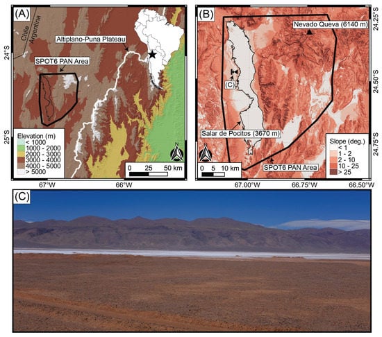
Figure 1.
The study area in northwestern Argentina: (A) topography from Copernicus 30 m DEM [32]. The eastern area of the map shows steep east-to-west gradients in topography to the drainage boundary of the hyperarid, internally drained Altiplano-Puna Plateau (shown in white), where elevation is ≥3000 m. SPOT6 panchromatic (PAN) area shows the stereo–data extent; (B) zoom on the SPOT6 data area centered on the Salar de Pocitos dry paleolake bed (salt flat) with steep surrounding mountains and a ∼2500 m elevation gradient between the salar (lowest elevation) and highest volcanic mountain (Nevado Queva). Slope map indicating the flat salar and steep mountains is derived from the Copernicus 30 m DEM; (C) photograph identified in (B), demonstrating the flat salar (photo taken on low–slope alluvial fan, white area in middle ground is salt flat), and the smooth, vegetation–free topography of the surrounding mountains characteristic of the study area, with localized bedrock outcrops and incised valleys.
3. Data and Methods
Our analysis is based on tristereo data from the SPOT6 satellite. The three overlapping optical scenes are processed using the ASP version 3.0 [25]. Previously used differential Global Navigation Satellite System (dGNSS) geodetic measurements [10] are also presented in the results section but primarily can be found in the Supplemental Material. The DEM quality and its relation to image texture is explored on the Salar de Pocitos. Finally, landscape curvature is used to compare results of different stereo matching algorithms and processing parameters for geomorphic applications.
3.1. SPOT6/7 Satellite Data
The SPOT6/7 satellites, launched in 2012 and 2014, offer high-resolution optical satellite imagery with a stereo and tristereo capacity. We work with a clip of a SPOT6 stereo triplet that covers an area of ∼2700 km (Figure 2A). All images were acquired from a single pass on 13 April 2014 and come as 12-bit panchromatic (PAN) scenes with a ground resolution of 1.5 m. The scenes are corrected for radiometric and sensor distortions but have not undergone any geometric correction or orthorectification (Level 1A format). To carry out the geometric correction autonomously, the user is provided with a set of Rational Polynomial Coefficients (RPCs). These replace a physical sensor model through a mathematical model that allows mapping the image-to-ground coordinates without revealing the intrinsic parameters of the sensor [22]. However, we do note that SPOT6/7 data are delivered with a rigorous sensor model in addition to RPC data [33], but only the RPCs can be read by the ASP, and these are the most general method of geometric correction for satellite data (e.g., WorldView, GeoEye, Planet). The stereoscopic acquisition mode of the SPOT6/7 satellites collects two or three images from different viewpoints which allows us to reconstruct the terrain through stereogrammetry. The acquisitions (herein labelled as scene A, B, and C) used in this study have the following along-track angles: A = −14.96 (southward view); B = 0.3 (near-nadir view); and C = 15.8 (northward view). With the satellite flying at a height of 694 km, the Base/Height (B:H) ratio for the AB and BC pair is ∼0.25 and ∼0.5 for the AC pair (Figure S1). The optimum B:H ratio for generating DEMs depends on the relief of the captured area. An increased B:H ratio is beneficial for matching large flat areas with little topography. Smaller B:H ratios reduce the ability to measure parallax between two features but also reduce the risk of having hidden areas in steep terrain. Greater similarity of the images from smaller B:H ratios can furthermore aid the stereo-matching process [33].
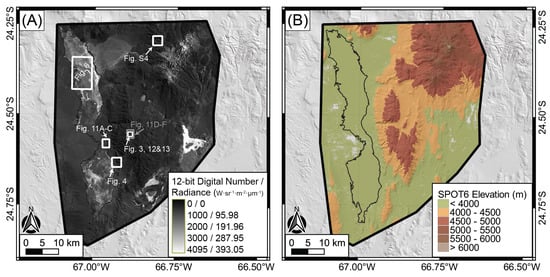
Figure 2.
Same area shown in Figure 1B overlain with SPOT6 data: (A) SPOT6 panchromatic (PAN) B-scene shown in grayscale as 12-bit digital numbers (values of 0-4095) and converted to top-of-atmosphere radiance (units of W/m/sr/m) by dividing the digital number by the gain constant value of 10.4186 and adding the bias constant value of 0, both found in the SPOT6 metadata. Note the spectral range of the SPOT6 PAN channel is 0.450–0.745 m. Boxes and labels indicate the areas of subsequent figures in the main text and Supplemental Material; (B) topography from SPOT6 DEM BM-ck25 (cf. Table 1) following ASP processing. Holes in the DEM are shown by gray colors, particularly prominent on alluvial fans where image texture is low.
3.2. DEM Generation with the Ames Stereo Pipeline
All SPOT6 tristereo scenes are processed in the ASP version 3.0 [25] using a custom pipeline to generate DEMs, such as the example shown in Figure 2B. A shell-script version of the processing is available on the GitHub page associated with this paper: https://github.com/UP-RS-ESP/Ames-Stereo-Pipeline-SPOT, last accessed 28 September 2022. The ASP is a flexible tool for DEM generation first developed by NASA’s Ames Research Center for the Mars Pathfinder Mission. It can handle robotic, satellite, aerial, and historical stereo imagery and is open-source, and mostly automated, requiring little manual input aside from initial pipeline design and testing [23,24,25]. Other studies have detailed the robustness and flexibility of the ASP for a variety of terrestrial satellite and aerial data for primarily cryospheric applications (e.g., [7,23,34,35]), and these studies are complementary to ours, which is concerned with snow- and ice-free mountain landscapes. We report on the main algorithms and parameters tested in this study, which can largely be found in the ASP manual: https://stereopipeline.readthedocs.io/en/latest/, last accessed 28 September 2022 [25]. We do not detail all of the myriad parameters in the ASP, but we do qualitatively mention some relevant tests we carried out. We conclude this section with step-by-step details of our pipeline, but we emphasize that similar findings and observations can be reproduced by other stereo-matching software packages.
3.2.1. Bundle Adjustment and Map-Projection
Prior to image correlation, camera or sensor parameters and positions need to be corrected and adjusted. This step is referred to as bundle adjustment and relies on correlating features in 2D image space and 3D object location: the least squares bundle adjustment minimizes the error between the 3D location of image features. This results in parameters stored in matrices containing the new camera orientations and positions, which are later used to improve the correlation and triangulation results. Self-consistent cameras also reduce blunders during stereo triangulation of point clouds.
In a second step, the left and right image of a given image pair are roughly aligned (i.e., rectified) to each other before correlation begins. In the classic computer vision approaches relying on images taken with optical cameras, this is often achieved by translating and rotating the images against each other to form a homography that generates epipolar lines across the images. This means that after the rotation and translation, points (pixels) on one row of a warped left image correspond exactly to the points along the same row in the warped right image. Finding matching pixel patterns only along the same row greatly increases computational efficiency. In the case of satellite or aerial imagery of a planetary surface, another option exists for initial left and right image rectification: map-projection. This is preferable for line-based scanners, such as most satellite images.
Map-projection takes each individual image (e.g., the SPOT6 A scene) and uses the results of the bundle adjustment step along with the associated RPC metadata from the scene to project the image onto a provided, often coarser (30 m), DEM. Rather than intersecting the SPOT6 images with each other for rectification in the classic computer vision method, map-projection intersects each image with the smooth DEM; both images are independently orthorectified resulting in a pair of similar images that differ only in small perspective differences, which are the features detected during stereo correlation. This is somewhat comparable to differential interferometric synthetic aperture radar approaches, where an interferogram is formed by removing the topographic phase from both radar scenes to end up with a cleaner deformation signal without the topographic component. A map-projection of the satellite or aerial images is strongly recommended, and an initial smooth DEM is required for the study area.
3.2.2. Stereo-Correlation Algorithms and Parameters
Stereo correlation, the process of matching pixels between overlapping images, is the main processing step in optical DEM generation in the ASP or any other software. The map of matching pixels is the disparity map, which contains the vertical and horizontal offsets from the right image pixels (usually treated as moving, or secondary) to the left image pixels (usually treated as reference, or primary). These disparity values between each overlapping pixel are refined and fed into a triangulation phase, where the depth is retrieved and eventually converted to the final elevation values. Many correlation algorithms exist, which were often originally developed in the computer vision communities and later applied to stereogrammetry, leading to further refinement and changes specific to the issues of stereo correlation for satellite imagery. Below, we detail the main popular algorithms that we tested, but we also refer the reader to studies describing the algorithms [36,37] and the ASP manual [25] section on stereo algorithms (https://stereopipeline.readthedocs.io/en/latest/stereo_algorithms.html, last accessed 28 September 2022). Unless mentioned, other processing parameters in the ASP remain at their default settings.
The most widely used and well studied [36] correlation algorithm is Block Matching (BM), and it is the default option in the ASP. In this approach, a small window of pixels centered on the pixel of interest is taken from the left image, and a corresponding window is passed locally over the right image to find the matching pixel to calculate the disparity. The window is referred to as the Correlation Kernel (CK) and is by default 25 × 25 pixels in size. The pixel selection is performed using a cost function calculated for all pixels, where the minimum cost is selected as the matching pixel. The BM algorithm uses the Normalized Cross Correlation (NCC) to obtain the pixel costs. This results in integer disparity values for all pixels which then need to be refined ina second step to obtain sub-pixel precision. During the sub-pixel refinement stage, a slightly larger Sub-pixel Kernel (SK) is centered on the initial disparity match to improve the pixel matches; however, rather than taking the cost function minimum, improvements are typically achieved using either parabola fitting to the correlation cost surface or a Bayes expectation maximum (Bayes EM) weighted affine adaptive window [25,38,39]. The SK defaults to 35 × 35 pixels for the BM algorithm.
The second correlation algorithm that we investigated in detail is known as More Global Matching (MGM). The MGM algorithm, developed by Facciolo et al. [40], is a slight improvement on the Semi-Global Matching (SGM) algorithm originally by Hirschmuller [37]. MGM differs significantly from the BM approach, in that it takes 8 cost pathways (original implementations can take 2, 4, 8, or 16 pathways) meeting symmetrically at the pixel of interest through the correlation search windows and is able to use much smaller CK and SK windows, both leading to improved matching in areas of low texture or repetitive features. For MGM, the cost function is not restricted to the classic NCC but can use census or ternary census [41] functions for each of the 8 cost pathways. Census cost functions maintain the local ordering of radiometric intensity in a given window, thus improving disparity matches in similar left and right image windows with differences in contrast. As opposed to a traditional census, a ternary census uses 2-bit encoding, and full details of the algorithm can be found in Hu et al. [41]. By default, the MGM CK is set to 7 × 7 pixels in the ASP, and the SK is set to 15 × 15 pixels. Many computer vision applications of SGM or MGM involve searching in 1D along epipolar lines from the rectified images. However, the ASP implements a 2D disparity search, which is more computationally expensive, but also more flexible and helps find matches in map-projected images when the alignment along the image y-axis (rows of pixels) is imperfect.
In initial tests using both the MGM and BM algorithms, we used a small clip of the full PAN SPOT6 images and processed them iteratively by changing parameters suggested in the ASP documentation, and in the online ASP forum: https://groups.google.com/g/ames-stereo-pipeline-support, last accessed 28 September 2022. The resulting DEMs were checked by visual inspection of the hillshade image and through differencing DEM and dGNSS heights measured within the study area (cf. Figure S2 for dGNSS coverage). We found that the Bayes EM sub-pixel refinement approach had the best results (least hillshade artifacts, lowest differences compared to dGNSS) and used this in all further runs. We also varied some key parameters associated with filtering matches for the MGM algorithm (median-filter, texture-smooth-size, texture-smooth-scale) but found minimal differences in the outputs even doubling or halving the defaults due to the high radiometric resolution of the SPOT6 imagery (12-bit), which leads to high texture. Overall, during initial testing, we found the largest difference in results from the size of the CK and SK and the cost function (NCC or ternary census) used. For the cost functions, the BM approach is limited to the NCC method, but we saw improvement in the MGM results when the NCC was exchanged for the ternary census. Additionally, in the ASP, the maximum allowable size of the MGM CK is 9 × 9 pixels when using the ternary census cost function [25]. These tests and limitations led us to a detailed investigation of six final DEMs generated with the parameters listed in Table 1. Our SK sizes were selected to follow the conventions of the defaults, which are +10 pixels for BM and approximately double for MGM. Varying the SK ±2–5 around these values did not change results appreciably.

Table 1.
Parameters and names used herein for the SPOT6 DEMs. All DEMs were generated using the AC pair and output to 3 m resolution; BM = Block Matching; MGM = More Global Matching; NCC = Normalized Cross Correlation; CK = Correlation Kernel; SK = Sub-pixel Kernel.
Thus far, we refer only to the correlation of image pairs (e.g., SPOT6 A and C scenes). The ASP can also accept three or more images (e.g., SPOT6 A, B, and C scenes) and carry out correlation using the chosen algorithm from the first image kept as reference to all other images. However, when using three or more images, the triangulation step takes a multi-view stereo approach, which provides worse results compared to pairwise stereo due to averaging of triangulated points from different image pairs in common locations [35]. Bhushan et al. [35] found that stereo quality is lowest along overlapping image boundaries, but these effects may be reduced with large-swath SPOT imagery. We report on the differences between pairwise runs (e.g., SPOT6 AB pair versus AC pair) in Section 4.
3.2.3. Example of ASP Processing and Outputs
While there is no theoretical limit to the output DEM resolution following stereo correlation and triangulation, the ASP documentation and some studies (e.g., [23,34]) suggest a 4× DEM output with respect to the input image resolution (1.5 m for SPOT6), with the goal of smoothing artifacts and improving DEM quality. Here, we seek to generate the highest possible resolution DEM to better represent geomorphically important features, such as ridge crests and valley bottoms [42], which represent process changes in the landscape. Thus, we output DEMs at 2× the input resolution (i.e., 3 m DEMs), but we also generate a 6, 12, and 24 m DEM (4, 8, and 16× input resolution) for the default BM-ck25 output for comparative purposes. Below, we detail our custom processing steps (the shell-script version can be found online: https://github.com/UP-RS-ESP/Ames-Stereo-Pipeline-SPOT, last accessed 28 September 2022):
- SPOT6 Level 1A images in their native, tiled format are converted to GeoTiffs with RPC information contained in the file header, using the external GDAL command gdal_translate.
- An initial bundle adjustment is carried out on all three (A, B, and C) images using the bundle_adjust tool. In this way, satellite positions and orientations are adjusted relative to each other to improve the self-consistency of observations in all three images.
- Stereo correlation is performed on the AC image pair with the parallel_stereo tool and default BM parameters. Since the images are not yet map-projected, the initial rectification is done using the default affine epipolar approach. This step results in a low-quality preliminary matching.
- A low-quality 3 m DEM is generated from the preliminary matching using the point2dem tool.
- The low-quality preliminary AC BM-ck25 DEM is aligned to a reference 30 m DEM using the pc_align tool. We use the Copernicus 30 m global DEM, as it is of highest available quality for the study area [10]. This results in improved alignment of the preliminary DEM with the smoothed topography. Alternatively, the low-resolution point cloud of matches obtained during bundle adjustment could be coarsely gridded and aligned to a reference DEM to avoid the initial stereo correlation and reduce processing time.
- Another run of bundle_adjust is performed on the original SPOT6 images, now passing the results of the first bundle adjustment and the results of the 30 m DEM alignment in the previous step as initial conditions for camera positioning. This results in additional improvements in camera positioning with respect to tie-points observed in each image and with the smoothed topography from the Copernicus DEM.
- Using the final bundle adjustment parameters from the previous step, each SPOT6 image (A, B, and C) is independently map-projected onto the reference 30 m DEM (Copernicus) using the mapproject tool. This results in orthorectified SPOT6 images in a WGS84 decimal degree projection with pixel resolutions of 1.5 m, equivalent to SPOT6 Level 2A data.
- The map-projected scenes are run pairwise (AC, AB, BC) through parallel_stereo using all tested algorithms and parameters. Each parallel_stereo output is converted to a 3 m DEM (or 6, 12, and 24 m for the BM-ck25 output) with point2dem.
The majority of the processing in Steps 1–7 insure the best possible map-projection of the images. Improved map-projection results in improved disparity searching and best-possible results in the final SPOT6 DEMs, which can be iteratively generated for many correlation algorithms and parameters in Step 8. Given the large size of the SPOT6 scenes (2700 km), all processing was carried out on a Linux server with 80 CPUs and 1 TB of RAM. Typical processing times for our ∼1.5 GB scenes were 10 to 20 h. Processing can be carried out on less powerful machines, but this requires the user to reduce the ASP tile size and memory limits (the corr-tile-size and corr-memory-limit-mb arguments passed to parallel_stereo) and would lead to longer computation times.
In addition to DEMs output by point2dem, we also retrieve the triangulation error map (a.k.a. the intersection error). The intersection error provides an indirect, relative metric of DEM quality at every pixel, measured as the shortest distance between the rays emanating from the pixel to each camera, with lower values indicating higher quality matching [21,24]. At any pixel where the intersection error exceeds the input image resolution (1.5 m), we constrain the point2dem tool to place a no data hole and do not interpolate these holes in our results. This is to avoid any interpolation artifacts and focus our results on the differences in stereo-correlation algorithms and parameters—including the number of holes.
3.3. Comparison of DEM Quality with Image Texture
Typically, DEM quality is assessed with external geodetic measurements by observing hillshade images and by other techniques looking at inter-pixel variability (e.g., [2,15]). Numerous studies detail statistical analyses of DEM quality (e.g., [3,43]), and here we present an approach unique to our study area that has the goal of demonstrating a chief cause of DEM quality difference between different algorithms and parameters: image texture.
Image texture, or the local difference in digital number values (converted to PAN radiance in Figure 2A using SPOT6 metadata), is known to cause issues with image correlation and has been defined mathematically in a number of ways (e.g., [26,41]). Some authors define image texture with respect to the orientation and magnitude of changes in pixel value (e.g., [44,45]). Here, we define image texture at a pixel independent of orientation as the variance of the PAN 12-bit digital numbers in a local window (3 × 3, 5 × 5, 7 × 7, or 9 × 9 pixels). Prior to calculation of the PAN variance, we resample the orthorectified (map-projected) PAN images to match the DEM resolution (e.g., 3 m), so that all pixel variances match between the PAN image and output DEM. For the texture calculation, we use only the SPOT6 B-scene as this is near the nadir, but results using the A or C scene are comparable.
In addition to the PAN variance variable, we also find the DEM variance in the same pixel window on the salar. The salar is locally a perfectly flat surface and should have near zero variability in height (cf. Figure 1C). To retrieve the matching DEM variance at a pixel, we employ a least squares plane fitting procedure in the same window (3 × 3, 5 × 5, 7 × 7, or 9 × 9 pixels) as the PAN variance and then calculate the point-to-plane distance of all elevation pixels in the window and take the variance of these distances. In effect, this corrects for any local tilting of the salar, and only looks at the erroneous height variations, which we assume should be near zero.
The combination of these variables on the salar allows us to explore the relationship between DEM quality (measured here as DEM variance on a flat surface, akin to the “runway” method of DEM quality estimation using flat airport runways [46]) and image texture (measured here as PAN variance) on a smooth, flat, vegetation-free surface. We note the salar has highly variable image texture due to 10–1000 m length-scale variations in salt patches and wind-blown dust.
3.4. Curvature Dependence on Matching Algorithms
Since most geomorphic studies are not concerned with flat surfaces, such as our salar, we use curvature as a proxy for examining DEM quality compared to a correlation algorithm and parameters on the off-salar (i.e., steeper) parts of our study area. Nevertheless, the DEM variance vs. PAN variance relationship from the salar does provide information on where higher and lower-quality results may be expected on the entire DEM. Aside from image texture issues, low-quality DEM results can also be caused by geometric issues with the satellite view angles compared to an object’s orientation, local processing blunders in the correlation, and systematic errors or biases caused by the sensor. We are not able to untangle or investigate all of these factors from our available data, but we can provide results to suggest optimal processing parameters for stereo matching to improve SPOT6 DEMs for geomorphic application.
To explore the DEM quality for geomorphic application, we calculate the landscape curvature in the mountainous parts of our study area. As the second derivative of elevation, curvature is highly sensitive to DEM noise. Since our study area contains diffusive and smooth, vegetation-free hillslopes, with only small, localized rocky outcrops (Figure 1C), spiky curvature across the landscape should be the result of lower-quality matches and not a true topographic signal.
Curvature was calculated in a 3 × 3 pixel window using the free and open-source LSDTopoTools software [47] on all DEMs projected to UTM coordinates with 3 m resolution. Many options exist for curvature [48], but here we choose the tangential curvature as output by LSDTopoTools via a quadratic-fitting approach [49]. This was selected since tangential curvature (measured perpendicular to the steepest topographic slope direction) is important for the identification and analysis of sharp features in the landscape (i.e., ridge crests, valley bottoms, channel heads), and we seek the DEM processing parameters that best preserve these features.
4. Results
We generated six DEMs (Table 1) using different processing parameters as described above. The quality of these results is assessed with respect to the following measures: absence of artifacts and voids, differences with respect to dGNSS reference data, the relationship between DEM variance and PAN variance on the salar, and sharpness of the landscape (i.e., the ability to preserve high curvatures). Unless otherwise noted, all DEMs are from the AC pairwise correlation. Section 4.3.1 deals with the alternative pairwise results from neighboring images (e.g., AB).
4.1. Visual Assessment of DEM Quality
Hillshaded images of the DEMs resulting from different correlation algorithms and parameters (Table 1) differ greatly (Figure 3). For either algorithm, increasing CKs correspond to a smoother surface. At the same time, voids in the output are reduced as larger and thus more distinct CKs aid the matching process. Reduced CK sizes appear to preserve sharper features in the landscape, which may be of interest to geomorphic studies looking at sharp ridge crests and valley bottoms. However, this occurs at the cost of a rising number of holes and apparent DEM noise due to false matches.
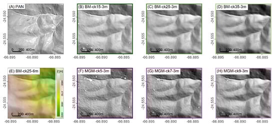
Figure 3.
Comparing the map-projected SPOT6 PAN B-scene (A) to the resulting stereo DEMs (Table 1) derived from AC pair; (B–D) hillshaded DEMs generated using the ASP BM algorithm at increasing CK sizes gridded to a 3 m resolution; (E) local topography with an elevation range of ∼500 m, taken from the DEM generated using the ASP default parameters and gridded to a 6 m resolution (4× input-image resolution); (F–H) the hillshaded DEMs based on the MGM algorithm with different CK sizes. See Figure 2A for location in study area. Green and purple frame colors correspond to colors in Figures 8 and 9.
DEMs generated with the BM algorithm are characterized by a surface with regular horizontally and vertically oriented artifacts, giving it a linen-cloth-like structure (Figure 3B–D). MGM artifacts can be described by a salt-and-pepper, or sandpaper, structure that is particularly apparent at low CK sizes (Figure 3F–H). Based on field knowledge, our hillshades should show smoothly varying topography (Figure 1C) and not the rough sandpaper-like appearance that becomes prominent with our smallest CK used for the MGM algorithm (5 × 5 CK size; Figure 1F). Such artifacts can be partially smoothed out by gridding the point cloud of pixel correspondences to a lower resolution (i.e., 6 m; Figure 3E), but this comes at the expense of losing smaller details and mixing DEM noise with reliable matches. A larger CK size also smooths these sandpaper-like artifacts, but as noted, this also smooths real sharp features (i.e., ridges and valleys).
A key difference we note between the BM and MGM algorithms is that the MGM results appear to better capture the particularly sharp (incised or eroded) portions of the study area, even at large CK sizes. In Figure 3, the deeply incised valleys are more clearly represented by the MGM DEMs, whereas they are increasingly smoothed out when using BM. This may be partially due to the larger CK sizes that the BM algorithm requires (CK sizes <15 × 15 were initially tested but led to many holes in the output DEM).
4.2. Comparison of DEM Heights to dGNSS Measurements
We compared SPOT6 DEM heights to dGNSS field measurements collected during field campaigns in 2015, 2016, 2017, and 2019. The validation of DEM heights with n ≈ 75,000 dGNSS points (accuracy <0.1 m horizontally and vertically) indicates that DEMs generated with large CKs are closer to the ground control (narrower distribution) than smaller CKs (Figure S3). For the BM algorithm, the normalized mean absolute deviation (NMAD), which measures the accuracy of the DEM elevations [43], ranges from 1.4 m (15 × 15 pixel CK) to 1.2 m (35 × 35 pixel CK); for MGM from 1.9 m (5 × 5 pixel CK) to 1.3 m (9 × 9 pixel CK). However, we do not consider the dGNSS difference as our primary indicator for DEM quality, as the absolute height difference does not reflect on the sharpness or smoothness of a landscape [15,21]. Furthermore, these reference points are limited to flat and easy-to-access parts of the study area (i.e., roads; Figure S2). Particularly flat areas are difficult to match without sufficient image texture. In these regions, a larger CK size is beneficial to reduce the number of false matches and artifacts. We suggest that the elevation comparison with dGNSS data reflects precisely this: in areas of low relief, a larger CK size producing a continuous smooth surface will better approximate ground truth. These observations, however, cannot be extrapolated to the steeper parts of the landscape, where larger CKs can blur complex features and average estimated 3D positions.
4.3. Image Texture as a Proxy for DEM Quality
In addition to hillshade images for an inter-DEM comparison, we examine the underlying SPOT6 PAN image texture (PAN variance calculated in a local window). We find strong correspondences between image texture and appearance of the resulting DEM. A side-by-side comparison of the PAN image, PAN variance, and hillshaded DEMs (Figure 4A–D) clearly shows that stereo correlation in the area of the texturally variable salar to the west yields a much smoother DEM surface. Here, the previously described linen-cloth-like structure inherent to the ASP BM algorithm is less apparent. In contrast, the homogeneous texture of the adjacent alluvial fan in the center relates to a much rougher part of the DEM. Here, stereo correlation is more likely to fail or produce false matches resulting in a larger number of artifacts and DEM noise (i.e., lower DEM quality). In regions with higher relief, this relationship between image texture and DEM quality is less distinct. Figure 4E,F also indicate that, in general, higher intersection error values also correspond to areas of lower PAN variance, although this is overprinted by horizontal banding caused by jitter of the SPOT6 satellite during flight, leading to pushbroom sensor artifacts.
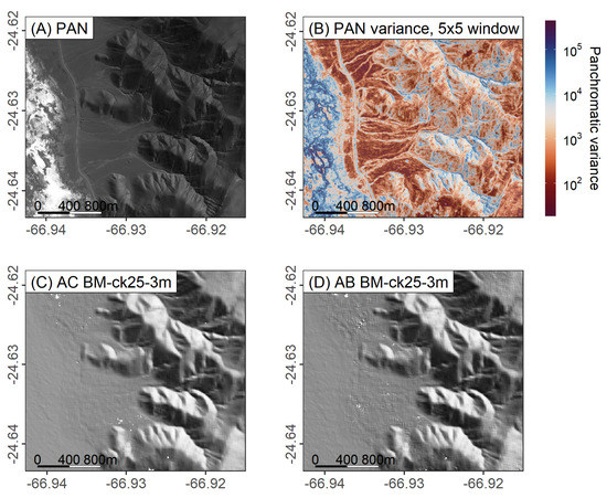
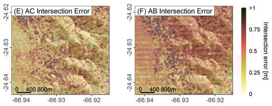
Figure 4.
(A) Map–projected SPOT6 PAN B–scene. The white color to the west is the edge of the salar (white is from salt patches), and there is an alluvial fan in the center of the view, which emanates from the steep mountains to the east; (B) the PAN variance calculated on (A) in a 5 × 5 window, and logarithmically scaled; (C) resulting SPOT6 DEM from pairwise correlation of the AC scenes and for the AB neighboring scenes (D); (E) Intersection error output by the ASP for the AC DEM and for the AB DEM (F); See Figure 2A for location in study area.
4.3.1. AC versus Neighboring Pairs
Comparing DEMs generated from neighboring pairs (AB/BC) and the pair with maximum view-angle difference (AC), we observe that neighboring pairs produce DEMs with more artifacts and a rougher surface (Figure 4C,D). The higher quality of the AC pair is further supported by the intersection error (Figure 4E,F): the AC pair has a much lower intersection error overall than the AB pair. The reason for this is the weaker stereo geometry of neighboring pairs—matching pixels/points from the AB pair cannot be triangulated as well due to a smaller parallax (disparity). The striped pattern of satellite jitter is also apparent, more so for the AB pair (Figure 4F) compared to the AC pair (Figure 4E). The decrease in DEM quality is also confirmed by the elevation differences to the dGNSS measurements (Figure S3C), where the NMAD values are 2.2 m (AB) and 1.5 m (BC) compared to 1.3 m for the AC pair.
Based on these findings, we conclude that the AC pair alone provided better DEM results than a mix of all pair combinations in this study area. Particularly, the low-sloping salar is better reconstructed through a larger B:H ratio, which is why we base subsequent analyses solely on DEMs generated from the AC pair. However, the nadir image is certainly useful when imaging deeply incised valleys or narrow alleys in urban areas where occlusions occur. This is highlighted in the Supplemental Figure S4, where the neighboring image pair (AB) shows a lower intersection error in the narrow valley bottom, while the oblique view images are not able to fully capture this area, resulting in more gaps in the final output. In such areas, combining the stereo correlation of AB, AC, and BC pairs may improve results.
4.3.2. Where Image Correlation Fails
Beyond visual assessments of hillshades and comparisons with local PAN variance, the holes associated with no-data values in the output SPOT6 DEMs provide insight into the performance of the algorithms and parameters. In Figure 5, we compare the PAN variance in pixels of no data to pixels with elevation values, and we compare the number of output holes with respect to both the stereo algorithms and output DEM resolution.
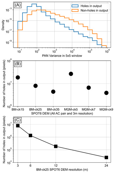
Figure 5.
(A) Comparison of PAN variance in DEM pixels with elevation values versus no-data holes (shown here for the BM-ck25 3 m DEM); (B) holes in output DEM for each of the 3 m DEMs generated from the AC image pair (cf. Table 1); (C) holes in output DEM for the BM-ck25 at 3, 6, 12, and 24 m resolution, which is 2, 4, 8, and 16× the input PAN image resolution, respectively.
In the comparison of 5 × 5 pixel window PAN variance in holes versus non-holes in the output AC BM-ck25 3 m DEM (Figure 5A), we note significant differences in the histograms: the distribution of PAN variance in the holes is skewed to lower values compared to non-holes. We remind the reader that holes in the SPOT6 DEM occur anywhere that the intersection error produced during stereo correlation exceeds the SPOT6 map-projected PAN resolution of 1.5 m. In other words, holes occur in the areas of highest stereo-correlation uncertainty, which Figure 5A shows is predominantly in the areas of lower PAN variance.
The differences in holes with respect to stereo algorithm and CK size are highlighted in Figure 5B. Most importantly, we see that as the CK size is increased, the number of holes decreases, which confirms the qualitative results in Figure 3. Additionally, increasing output resolution—as performed in the point2dem function of the ASP following stereo correlation and triangulation—significantly decreases the number of holes (Figure 5C). Of interest to the question of neighboring versus widest view-angle pairs, Figure S5 in the Supplemental Material depicts the decrease in holes in the AB and BC DEMs compared to the AC output. This is because the neighboring images are more similar and have fewer occlusions; thus, they can match more pixels, but, as previously noted, the parallax is smaller, and triangulation suffers.
4.3.3. Flat-Area DEM Variance versus Image Texture
The impression of PAN variance (i.e., image texture) compared to DEM quality as viewed in hillshaded images (Figure 4) and the lower PAN variance in output DEM holes (Figure 5A) lead us to a quantitative analysis of PAN variance versus DEM quality measured on the flat-lying salar. We emphasize that this unique, perfectly flat surface in our study area allows us to extract DEM quality as measured by DEM variance in local, plane-detrended windows matching the windows for PAN variance calculation. In Figure 6A, we selected a 2000 × 3000 pixel clip of the PAN B image from the central salar. Each pixel is 3 m resolution, where the orthorectified PAN B-scene was resampled from the original 1.5 m to match the output SPOT6 DEM resolution, and the number of pixels analyzed excluding holes in the DEM is ∼6 × , or an area of ∼54 km. The PAN variance, calculated here in a 5 × 5 window, spans ∼5 orders of magnitude due to variations in salt patches and wind-blown dust on the salar, providing a large range for comparison (Figure 6B). The DEM variance, also in a 5 × 5 pixel window, spans ∼5 orders of magnitude (Figure 6C) showing the large variability in DEM quality on the flat salar.
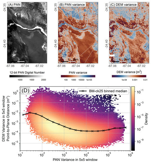
Figure 6.
(A) 2000 × 3000 pixel (6000 × 9000 m) clip of the SPOT6 PAN B-scene from the central salar (cf. Figure 2A). Grayscale variations (image texture) caused by salt and wind-blown dust; (B) variance calculated in a 5 × 5 pixel window from the original PAN scene; (C) DEM variance for the SPOT6 BM-ck25 3 m DEM, also calculated in a 5 × 5 pixel window using plane-fitting and the variance of point-to-plane distances. Note the reversed color scales in (B) (low to high, red to blue) compared to (C) (low to high, blue to red), in order to highlight the fact that lower PAN variance values (red colors in (B)) correspond to higher DEM variance values (red colors in (C)), and vice versa; (D) the variables shown in map view in (B,C) plotted graphically using a 2D histogram to highlight density of the ∼6 × underlying pixels (not plotted), as well as median bins calculated from all pixels.
The map-view comparison in Figure 6B,C is plotted graphically in Figure 6D. DEM variance is in units of m, but this can be viewed as a standard deviation uncertainty measurement (i.e., the variability of height in the window) by taking the square root. For instance, , , , , and m DEM variance are equivalent to standard deviation DEM uncertainties of 1, 0.3, 0.1, 0.03, and 0.01 m, respectively. Rather than plotting every DEM variance (y-axis) and PAN variance (x-axis) pixel value, we instead use a 2D histogram to represent the point density. A clear, banana-like shape emerges from the densest part of this 2D histogram (brightest colors), and plotting a binned median taken from all pixels (not plotted) further confirms this overall pattern in the DEM variance vs. PAN variance relationship. At PAN variances of ∼10–10, there is a continual decrease in DEM variance, but this begins to plateau around PAN variance, where we do not see continual improvement in DEM quality (further decreasing DEM variance).
The scattered nature of the relationship between DEM variance and PAN variance is apparent in Figure 6D by the wide spread of the 2D histogram. The density is logarithmically scaled, and we see that darker parts of the 2D histogram are several orders of magnitude less common; nevertheless, the densest area still exhibits significant spread across values. Thus, to better characterize the relationship between our variables, we employ an additional smoothing step, achieved by blocking the map-view PAN variance and DEM variance in 50 × 50 pixel areas, and obtaining the median value in these blocks (Figure 7A,B). Following this, the median values are plotted graphically for all blocks (∼2400 values), and a binned median is taken through these blocked points (Figure 7D). Under this smoothing, the banana shape of the relationship becomes apparent, with a steeply dipping improvement in DEM quality (DEM variance) with increasing image texture (PAN variance) that plateaus at high image texture.
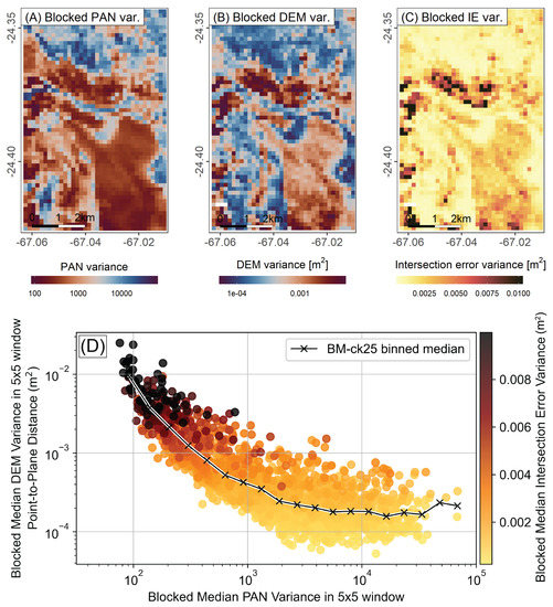
Figure 7.
(A) 5 × 5 pixel windowed PAN variance and (B) 5 × 5 pixel windowed DEM variance for the SPOT6 BM-ck25 3 m DEM, both blocked into 50 × 50 pixel (150 × 150 m) areas, with the median value in each block given by the color scale; (C) the same 5 × 5 pixel variance calculation and blocking carried out on the intersection error output from the ASP; (D) the blocked variables in (A) and (B) plotted against each other and colored by (C), with a binned median taken through all ∼2400 blocks.
We further highlight the relationship between PAN variance, DEM variance, and the intersection error (shown as blocked values in Figure 7C), by coloring the points by intersection error variance in each block (Figure 7D). We use the variance of intersection error rather than the raw intersection error for consistency with our other variance variables plotted. The point here is to highlight that areas of lower PAN variance and higher DEM variance (i.e., lower-quality parts of the DEM) are also associated with a mix of very high and very low intersection error values (high intersection error variance). This further emphasizes the high stereo-correlation uncertainties and resulting lower DEM quality in areas of low image texture and confirms observations made on the maps and hillshades in Figure 4.
When reducing the scatter by blocking and taking a binned median line as in Figure 7D for all SPOT6 DEMs (Table 1), the parameter’s relationships can be plotted together to view differences between stereo-matching algorithms and processing parameters. This is shown in Figure 8 for the DEM and PAN variance calculations in a 5 × 5 pixel window. These relationships are almost identical (only translated within ∼1 order of magnitude on the x- and y-axes) for 3 × 3, 7 × 7, or 9 × 9 window calculations. We note the reduction in DEM variance (i.e., improvement in quality on the flat salar) as the CK size is increased for both the BM (Figure 8A) and MGM (Figure 8B) algorithms. The BM algorithm also has a much steeper decrease in DEM variance with increasing PAN variance, exhibiting the plateau at ∼10 PAN variance across all tested CK sizes. On the other hand, the MGM approach exhibits a more gentle (less steep) shape, but we do still observe a slight breakpoint in slope at ∼10 PAN variance, followed by a plateauing behavior. For the MGM-ck5 DEM (the smallest CK tested), the DEM variance never falls below 10 m (0.03 m standard deviation).
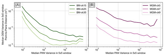
Figure 8.
Median binned line generated in Figure 7D for BM-ck25, here shown for (A) all BM DEMs and (B) all MGM DEMs (cf. Table 1). The BM algorithm has a more steeply dipping relationship, but both BM and MGM have a plateauing behavior above ∼10 PAN variance. Larger CK sizes preserve the shape of the relationship but result in lower DEM variance for the same PAN variance.
4.4. Curvature Distributions
To investigate the effect of differing ASP algorithms and parameters on the mountainous parts of the landscape, we plot the distributions of tangential curvature for all SPOT6 DEMs (Figure 9). From the distribution of curvatures from 0–0.5 m in Figure 9A, we see that the 6 m DEM (output from the BM-ck25 run) has lower magnitudes compared to the 3 m DEMs, all of which follow a similar pattern. For Figure 9B, the MGM-ck5 DEM has significantly higher magnitude curvatures compared to the larger CK runs (7 × 7 and 9 × 9 pixel windows). However, curvatures >0.05 m represent the >99th (often >99.9th) percentile for all DEMs, indicating that these may largely be noise in the DEM, localized sheer cliffs, rocky outcrops, or road cuts. Therefore, we zoom in on the 0–0.05 m range in Figure 9C,D. Here, we clearly observe for both algorithms that increasing the CK size leads to lower magnitude curvature distributions.
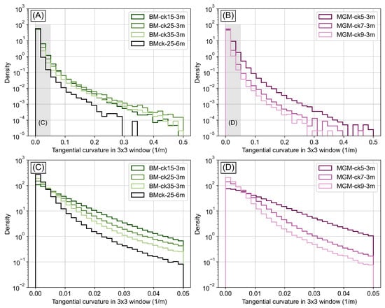
Figure 9.
Distributions of tangential curvature calculated in a 3 × 3 pixel window for the entire area of DEMs (including mountains in the study area; cf. Figure 1B). Distribution in the 0–0.5 m range for (A) BM results and (B) MGM results, with gray bar showing the 0–0.05 m zoomed areas in (C) for the BM results and (D) for the MGM results.
The higher curvatures observed with smaller CK may be the result of higher DEM variability (i.e., DEM noise) leading to spiky curvature measurements. However, we cannot preclude that these higher curvatures are not also caused by the ability of a smaller CK to preserve finer features, such as sharp ridge crests and valley bottoms, where curvature is expected to peak. This is further investigated in the discussion section, where we highlight noise versus signal for the various SPOT6 DEMs produced.
5. Discussion
Hillshade images, comparisons between DEM quality and input PAN image texture, and landscape curvature allow us to characterize differences in SPOT6 DEMs derived from the ASP using different stereo-correlation algorithms and parameters. In the ensuing discussion, we utilize our salar-based observations of DEM variance vs. PAN variance to generate relative DEM quality maps, which are based only on input image texture. We then discuss in more detail the implications of our different DEM outputs for geomorphic application, returning to curvature and looking at the results in map view. Finally, we report ideal processing steps and parameters for SPOT6/7 data in the ASP and mention caveats of the processing.
We note, although our dGNSS data (Figures S2 and S3) provides an initial quality assessment, these data do not present the full picture of DEM quality for geomorphic applications, since they are mostly restricted to flat roads and do not highlight the issues with elevation derivatives or inter-pixel consistency (cf. [15]). In addition, our SPOT DEMs are initially aligned to the Copernicus Global DEM; therefore dGNSS uncertainties related to Copernicus will be propagated to our SPOT DEMs. We expect the high-quality Copernicus DEM to closely match our dGNSS data, but propagating uncertainty effects are difficult to account for. We could have used a subset of the dGNSS in either bundle_adjust or pc_align and then compared SPOT DEM heights with the remaining dGNSS points, but the selection and placement of these points is challenging in our large, rugged study area. Because of these considerations, we only present our dGNSS data in the Supplemental Material to focus attention on other measures of DEM quality here.
5.1. Predicting DEM Quality from Image Texture
We are able to build a quantitative relationship between optical DEM quality and image texture on the flat, multi-textured salar surface unique to our study area (Figure 6, Figure 7 and Figure 8). As expected, areas with lower image texture (i.e., ⪅10 PAN variance) had lower-quality DEM results (i.e., a rough surface, whereas the true salar is smooth and flat). In the following, we present further analysis of this relationship in order to generate maps of DEM quality (i.e., per-pixel DEM uncertainty maps) from input images alone.
One way to analyze the banana plots in Figure 8 would be fitting functional relationships to the lines (e.g., exponential, powerlaw, etc.) to generate a predictive model of DEM quality. However, model selection and parameter tuning is a complex process, and the model will likely differ between correlation algorithms (differently shaped relationships). Furthermore, the observed relationship may be specific to our data (SPOT6 1.5 m PAN images) and study area. Given these caveats, we instead choose a simple approach to this analysis by fitting a piecewise function made up of two linear segments. This was chosen based on the graphical view of the relationships, where we observe a steeply dipping curve followed by a plateauing behavior in Figure 8 (noting the log-scaled y-axis). We seek an approximate breakpoint (location where two linear segments meet) in the PAN variance, below which DEM quality is increasingly worse and above which quality from image texture alone is high (i.e., correlation between images has high accuracy).
The piecewise fitting breakpoint analysis is demonstrated in Figure 10 for the BM-ck25 3 m DEM. For this, we take the blocked values shown in Figure 7D and iterate over them in a bootstrapping approach that provides us with a distribution of breakpoints. This is performed for each of the pixel window variance calculations (3 × 3, 5 × 5, 7 × 7, and 9 × 9), resulting in an even larger distribution of potential PAN variance breakpoints to choose from (Figure 10B). From this distribution, we selected the median value (rounded to the nearest hundred), which was 1300 PAN variance.
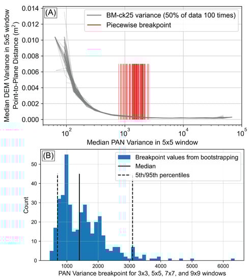
Figure 10.
(A) Piecewise fitting, using two linear segments, carried out on 50% of blocked values shown in Figure 7D, bootstrapped 100 times (with replacement). The vertical red lines represent the breakpoints found in each fitting iteration. Results are shown for the BM-ck25 DEM and 5 × 5 pixel variance window calculations. Note a linear y-scale is used here (as opposed to the logarithmic scale in Figure 8) to highlight the steep limb and plateau in the piecewise fitted relationship; (B) histogram of breakpoints taken from all variance window sizes (3 × 3, 5 × 5, 7 × 7, and 9 × 9 pixels) and iterations of piecewise fitting (n = 400 breakpoints), with median (1300 PAN variance) and 5th/95th percentiles identified.
Using this PAN variance value as our breakpoint, we are able to generate DEM quality maps from the input image alone, both on the salar (Figure 11A–C) and off-salar in the mountainous parts of our study area (Figure 11D–F). Given the shape of the relationship between DEM variance and PAN variance on the salar, we may expect that all PAN variance values above 1300 would lead to high-quality DEM results because this is where the DEM quality begins to plateau (Figure 10A), and further improvements in local standard deviation are ≪0.03 m. On the other hand, as we move farther below 1300 PAN variance, DEM quality rapidly degrades in the steep limb of the relationship shown in Figure 10A. Thus, in Figure 11, the solid blue color indicates values above our PAN variance breakpoint (higher expected DEM quality), and the shades of red indicate values below (lower expected DEM quality).
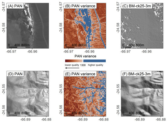
Figure 11.
Relative DEM quality maps based on the PAN variance breakpoint found in Figure 10B: (A) map-projected SPOT6 PAN B-scene from an area bordering the salar. (B) 5 × 5 pixel window PAN variance for the same region, with the color bar centered on the breakpoint value (1300 PAN variance). Red colors indicate lower DEM quality (increasingly worse, as shown by the arrow), and the solid blue color indicates higher DEM quality (plateau in DEM variance vs. PAN variance relationship in Figure 10A; (C) hillshade from the same salar area for the BM-ck25 DEM; (D–F) the same results shown for a more mountainous part of the study area. See Figure 2A for location in study area.
These quality differences are clear on the salar in a hillshade view (Figure 11C), where there is a much rougher surface and more holes observable in the low PAN variance areas (red colors in Figure 11B). On the other hand, in the mountainous terrain the difference is more subtle to observe, but, from the quality map in Figure 11E, it appears that the more highly textured ridges and valley areas may be expected to have higher quality DEM results (solid blue color), whereas many hillslopes have lower texture and thus worse DEM results. Taking the mode of the histogram in Figure 10B would provide a value of 1000 (our previously quoted 10), but the 5th–95th percentiles of breakpoint values fall between ∼800–3000 (i.e., within ∼1 order of magnitude) and moving the breakpoint in this range does not have an appreciable effect on resulting map quality (noting that PAN variance can generally cover a range of 5+ orders of magnitude in our study area but has no theoretical limit).
In this discussion, the breakpoint analysis and quality maps only offer a relative view of DEM quality, complementary to the intersection error map produced by the ASP following stereo correlation. We only present results for the BM-ck25 3 m DEM, since it is closest to the default parameter ASP output, but we note that a similar breakpoint analysis on the other SPOT6 DEMs produced similar values near 10 PAN variance. This method ignores other causes of poor DEM quality, such as geometric issues with the terrain compared to satellite view angles, and reduces quality entirely to the input image texture. It is highly unlikely that image texture alone impacts DEM quality, and many other factors also influence the results (e.g., striping pattern of the intersection error in Figure 4 caused by sensor and satellite motion).
In an attempt to elucidate these other issues and present a method for DEM quality assessment in study areas that may not have a large, flat, multi-textured surface such as our salar, we also tried to form a DEM variance versus PAN variance relationship off of the salar. We found that even when using very small (3 × 3 pixel, or 9 × 9 m) windows for the DEM variance calculation via plane fitting, the influence of true topographic signal (hillslopes in our study area are rarely perfectly planar at the 9 × 9 m scale), overprints the DEM variance versus PAN variance relationship (Figure S6), making a breakpoint analysis infeasible on non-flat terrain.
Despite these caveats, the breakpoint and quality maps presented here may serve as starting points for future research seeking to disentangle quality issues on optical DEMs produced via stereo correlation. It is clear that image texture has a very large influence on the quality of DEMs produced via stereo correlation, as qualitatively observed by many authors (e.g., [22,27,35,40]). We suggest that at local (3 × 3–9 × 9 pixels) image variance values ⪅10, stereo correlation has rapidly degrading results. Above this approximate threshold, remaining DEM quality issues are independent of image texture (e.g., may be caused by sensor biases or geometric issues).
5.2. Implications for Geomorphic Analysis
Our analysis of DEM quality with respect to image texture is restricted to the flat salar. Here, quality suffers primarily from lack of image texture, leading to correlation blunders across all algorithms and parameters. Although increasing the CK size appears to reduce DEM variance (improve DEM quality) on the flat salar, we also see that these larger CKs smooth the landscape and reduce high curvatures (Figure 9). However, the question remains: where are these high curvatures actually occurring on the landscape, and do their spatial patterns inform us on the DEM quality for geomorphic applications from the different algorithms and parameters?
Figure 11D–E show that there is higher PAN variance in valleys, ridges, and even on some hillslopes, which indicates higher quality DEM results in these geomorphically relevant locations. Higher image texture here is caused by erosive features and lighting differences at these areas of high curvature and changing aspect. This is a good sign, and to answer the posed question in greater detail, we analyze the noise patterns in the tangential curvature. Our study area is geomorphically smooth, with only localized rocky outcrops and no vegetation that could lead to widespread rough optical DEM texture (Figure 1). Therefore, high curvatures should mostly be restricted to ridge crests and valley bottoms.
To identify the high curvature locations, we took the 3 × 3 pixel window tangential curvature map for each SPOT6 DEM and differenced it with a Gaussian-smoothed (standard deviation of 1 and cutoff at 5 × 5 pixels) version of itself. In Figure 12, we observe orthogonal (approximately N-S and E-W oriented) artifacts in the BM algorithm (the linen-cloth hillshade texture previously referenced), which obscure the ridge and valley high curvature areas. These artifacts are somewhat reduced (lower magnitude difference compared to the Gaussian-smoothed version) at larger CK sizes (Figure 12F) but are still visible, and there are still many high curvature areas apparent on smooth hillslopes. In the MGM results (Figure 13), we see the smallest CK (5 × 5 pixels. Figure 13B) produces many localized blunders (spikes and pits shown as dark salt-and-pepper colors scattered randomly). However, going up to the 9 × 9 pixel CK (Figure 13F), these blunders are smoothed, and the darker colors (high curvature) in deeply incised valleys become apparent, with minimal high curvatures on hillslopes. This implies that the MGM is producing a less noisy, more geomorphically useful result, particularly with a larger CK in our landscape, where the hillslopes have lower texture (Figure 11E). For a side-by-side comparison of the curvature differences for the two matching algorithms, see Figure S7.
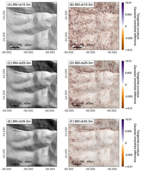
Figure 12.
Difference between tangential curvature calculated in a 3 × 3 pixel window and a Gaussian-smoothed version of this curvature map for the BM DEMs. Same area as is shown in Figure 3 (see Figure 2A for location in study area); (A) hillshade of the BM DEM with a CK of 15 × 15 pixels; (B) curvature difference map for this DEM. Larger differences occur in areas with more spiky DEM curvature; (C–F) similar pairwise (hillshade and curvature difference) results for the CK 25 × 25 and 35 × 35 pixel BM DEMs.
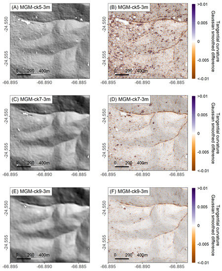
Figure 13.
Difference between tangential curvature calculated in a 3 × 3 pixel window and a Gaussian-smoothed version of this curvature map for the MGM DEMs. Same area as is shown in Figure 3 (see Figure 2A for location in study area); (A) hillshade of the MGM DEM with a CK of 5 × 5 pixels; (B) curvature difference map for this DEM. Larger differences occur in areas with more spiky DEM curvature; (C–F) similar pairwise (hillshade and curvature difference) results for the CK 7 × 7 and 9 × 9 pixel MGM DEMs.
The finer features identified with a smaller CK used in the MGM algorithm are in agreement with Dehecq et al. [34], who also noted similar blunders (spikes and pits) in DEMs produced with the MGM approach in low-texture areas where the algorithm interpolates disparity values. We cannot say what the true landscape curvature is without additional data (e.g., lidar), but we can say that there is a trade-off between smoothing and identifying the sharper features in the landscape, and the MGM algorithm appears (from the curvature difference map view) to better identify ridges and valleys, where we know the highest curvatures should be in the absence of bedrock outcrops or other high-curvature hillslope features. It is well-known that higher resolution DEMs (e.g., from lidar) are able to discern finer scale features of geomorphic interest (e.g., [42,50,51,52,53,54,55]); thus, the limits of satellite data should continue to be pressed.
Studies comparing high-resolution (i.e., ≤5 m) optical satellite DEM quality for geomorphic applications are few; DEM generation is typically carried out in less flexible software compared to the ASP, and processing parameters are not analyzed in detail (e.g., [6]). A notable exception is the recent work of Atwood and West [56], who used the Surface Extraction from TIN Space-search Minimization (SETSM; [57])—an alternative algorithm to those contained in the ASP—to generate WorldView DEMs at 2 m resolution for geomorphic application. These authors found high quality from these stereo DEMs, and similarly evaluated the quality based on derivatives of elevation, such as slope and curvature. This work, along with our previous [21] and present study, may serve as a basis for future work seeking to optimize optical DEM quality for geomorphic applications in mountainous regions. Optical satellite data have a rich and growing archive and are valuable data sources for Earth surface analyses. Additionally, the remote sensing and computer vision communities continue to develop and improve algorithms for high-quality depth retrieval from overlapping images. Higher resolution satellites (e.g., ≤0.5 m, such as those used by Atwood and West [56]) will likely contribute to vastly improved DEM quality given the increase in image texture that comes with the ability to discern finer features compared to the 1.5 m resolution data used here. Optical DEMs will also be affected by land cover, particularly vegetation, but these effects are avoided in our bare-Earth study area in order to isolate the image-texture uncertainty component. Future studies in vegetated regions could use these findings as a starting point for uncertainty analyses.
5.3. Best Practices for Generating DEMs in Ames for SPOT6/7
Recent studies using the ASP highlight some key parameters for DEM generation. These studies had cryospheric applications, seeking to measure changes in snow and ice on time series of optically derived DEMs from satellites including: sub-meter ∼0.3–0.9 m WorldView, GeoEye, Quickbird, and Planet SkySat-C [7,23,35]; 15 m ASTER [7,58]; and ∼6 m declassified KH-9 Hexagon data [34]. This work, in addition to our previous experiences with SPOT7 data in the ASP in a nearby region [21], guided our initial parameter selection, with a focus on vegetation- and ice-free mountainous terrain. Our results extend to SPOT7 data (the twin satellite to SPOT6) and may be generalized to other imagery used in steep mountain studies.
Orthorectification (map-projection) is a vital step prior to stereo correlation, and, in line with other work (e.g., [21,23,34]), we found dramatic improvements using our orthorectification processing detailed in Steps 1–7 in Section 3.2.3. These steps are similar to those in Dehecq et al. [34], who found that careful map-projection of KH-9 historical spy images increased DEM coverage by reducing the parallax (i.e., disparity) on features identified in overlapping scenes. A pair of GIFs on the GitHub repository associated with our work (https://github.com/UP-RS-ESP/Ames-Stereo-Pipeline-SPOT, last accessed 28 September 2022) depict the result of map-projection and the parallax between two map-projected scenes. Recent work by Bhushan et al. [35] and Dehecq et al. [34] have highlighted improvements when using the MGM algorithm compared to BM, and here we further investigated the cost functions used in these algorithms (NCC, census, ternary census) and found that the ternary census algorithm (which can only be used in MGM processing and preserves radiometric intensity ordering) leads to high-quality results (smoother DEM, less artifacts, lower difference to dGNSS). We note that Dehecq et al. [34] referred to NCC as a correlation algorithm, but this is rather a processing parameter (cost function) that lies at the heart of the BM stereo-correlation algorithm. We did not test the stddev filter in point2dem (which follows stereo correlation) as in the work of Dehecq et al. [34], since their study used this filter to bring out low-texture regions in images from Hexagon, which had a low 8-bit radiometric resolution.
In agreement with previous work, the most important selection in stereo correlation, aside from the algorithm and cost function, is the CK size [34,35]. While the CK size is not directly comparable between the two algorithms (BM and MGM) and therefore does not represent a true continuum of sizes (because the algorithms differ significantly), it should be noted that the most holes are produced by the smallest CK (5 × 5 pixels for MGM; Figure 5B). Furthermore, Figure 5C demonstrates that in addition to larger CK sizes, which improve correlation in areas of lower texture (lower PAN variance; Figure 8), a similar effect (smoother DEM with fewer holes) can be achieved by outputting the correlation and triangulation results at a coarser resolution. However, the coarser resolution output by the point2dem tool has no effect on the stereo correlation, which is always performed for every overlapping pixel at the input PAN image resolution (cf. ASP manual; [25]). Rather, these different output resolutions represent different averaging of the triangulated values at every pixel. In essence, naively outputting the DEM at a coarser resolution (e.g., here 6 m, or 4× the input resolution), has the effect of smoothing results and reducing artifacts [23], but this can also be achieved using larger CK sizes and outputting a finer DEM (e.g., here 3 m, or 2× the input resolution). Larger CKs have been suggested by previous studies in areas of low image texture (i.e., glaciers and ice-sheets; [34,35]), and we find quantitative evidence for this through our salar analysis (Figure 8). Further, we found that for our study area with low texture (i.e., ⪅10) on many hillslopes (Figure 11E), larger CK sizes in the MGM algorithm led to smoother DEMs that better represented high curvatures in valley bottoms compared to smooth hillslopes (Figure 13F).
An ASP parameter that we have not yet mentioned is the xcorr-threshold, which allows stereo correlation to proceed for the left image as reference and then again for the right image as reference, doubling processing time. Similar to previous work [23,34], we found significant improvements from allowing both correlation directions to refine the disparity map, and this is recommended for the highest quality results.
Finally, similar to previous work (e.g., [35,59]), we found that the highest quality correlation and triangulation results can be achieved from image pairs with a larger convergence angle (e.g., AC). Utilizing neighboring pairs of tristereo imagery (e.g., AB) may improve coverage in steep canyons (Figure S4) or urban areas with tall buildings that cause occlusions, but blending these results into final DEMs is not recommended in other locations. This is in contrast to the ASP manual [25], which suggests using the pc_merge and/or dem_mosaic tools to blend results from different image pairs. We note that the nadir scene was used in our previous work [21] in an area with very steep mountains and incised gorges, but blending outside of these gorges may have reduced the final quality. This may benefit future research in mountain environments where there are limited steep bedrock gorges, since the nadir tristereo image does not need to be acquired (i.e., purchased), and just the forward and backward pointing scenes may be sufficient. In agreement with other work [59], this demonstrates that the optimal image pairs with a larger difference in viewing angle will lead to better quality elevation measurements, and stacking many optimal image pairs with good geometry (even if the images are from different dates) may lead to further improved results.
We found that the overall flexibility of the ASP, including its incorporation and refinement of many stereo-correlation algorithms and their parameters, make this open-source software a suitable tool for optical DEM generation. We note that other recently presented techniques offer somewhat less flexibility and more specific applications, e.g., MicMac [14], SETSM [56,57], and Metashape software [60]. Continued development of structure-from-motion multiview stereo (SfM-MVS) methods may lead to satellite DEMs generated from vastly different pipelines compared to traditional stereogrammetry [22]; but, SfM-MVS results for satellite stereo imagery are still nascent and of generally lower quality compared to using carefully selected image pairs for stereo correlation [35,59,61]. Indeed, we found that initial tests of DEM generation using Agisoft Metashape [62] led to poor results, albeit in much faster processing times and with fewer parameters to tune compared to the ASP. Future studies of optical DEMs could benefit from a rigorous quality analysis using advanced statistical approaches (e.g., [3]); however, this requires reference DEMs (e.g., from high-quality lidar datasets), which were not available in the present study.
6. Conclusions
Optical satellite images from SPOT6/7 (tri)stereo, and other similar <2 m resolution satellites, offer a rich trove of past and ongoing Earth observations from which elevation models can be derived. These DEMs suffer from many errors (both systematic and random), which are concerning for geomorphic applications seeking to analyze fine landscape features such as ridges and valleys. Quality issues can be partly mitigated by carefully chosen processing steps, including appropriate software, pre-processing, stereo-correlation algorithm, and parameters. In this study, we have used the open-source Ames Stereo Pipeline [23,24,25] to generate DEMs from SPOT6 tristereo imagery on a smooth, mountainous, vegetation-free study area. Our ASP results extend to other software that uses similar algorithms and parameters. We can summarize our findings in the following:
- The unique salar (salt flat) in our study area allowed us to explore the relationship between image texture and DEM uncertainty. Higher image texture (measured by local panchromatic variance) improved DEM quality due to better stereo matching up to a certain point (∼10 panchromatic variance), beyond which other factors such as satellite view geometry and sensor biases may dominate.
- Compared to the Block Matching stereo-correlation algorithm, the More-Global Matching algorithm (with the ternary census cost function) preserved smaller scale features using smaller correlation kernels and had improved matching in low-texture areas.
- Larger correlation kernels improved matching (less holes) at the cost of smoothing the landscape. Increasing the kernel size will lead to more reliable matches and the ability to output a DEM at 2× the input image resolution and should be preferred in geomorphic applications to a naive smoothing by downsampling the final DEM to 4× the input image resolution.
- Using only the AC image pair (widest view-angle difference) for stereo-DEM generation produced higher-quality results than using the neighboring (AB, BC) pairs with the nadir scene (B). Mixing them (e.g., by median blending) likely degrades overall quality. However, the neighboring pairs with the nadir image are useful for filling holes (e.g., in steep canyons with occluded views). Images with optimal, wide viewing angles (even if they are from different dates) are therefore recommended for high-quality DEM generation.
- The higher curvature that we found using a smaller correlation kernel available in the More-Global Matching algorithm (9 × 9 pixels) likely demonstrates the preservation of landscape sharpness. Smaller kernels may also preserve even finer features, but this comes at the expense of more noise on hillslopes and other low-texture areas.
Taken together, our findings show a path forward for optical DEM fusion, whereby different parts of the landscape have different processing parameters (e.g., adaptive correlation kernels in areas of low vs. high image texture, use of the nadir image in areas with steep gorges). However, we did not present such a DEM fusion method here (e.g., using several outputs from different parameters), as this is beyond the scope of the current study. Overall, we find that the Ames Stereo Pipeline is a very suitable tool for the generation of optical DEMs for geomorphic applications and encourage the wider community of topographic data users to adopt it for their research.
Supplementary Materials
The following supporting information can be downloaded at: https://www.mdpi.com/article/10.3390/rs15010085/s1.
Author Contributions
Conceptualization, B.P. and B.B.; methodology, B.P., B.B. and A.M.; formal analysis and investigation, B.P.; resources, B.B.; data curation, B.P.; writing—original draft preparation, B.P. and A.M.; writing—review and editing, B.P., A.M. and B.B.; visualization, B.P. and A.M. All authors have read and agreed to the published version of the manuscript.
Funding
The SPOT6 tristereo scenes were received by B.P. from the ESA Third Party Mission project proposal ID 67754. Additional funding was sourced from DFG BO 2933/3-1 (B.B.), DFG funded IRTG-StRATEGy (IGK 2018) to M.R. Strecker and B.B., and BMBF LIDAR and NEXUS funded through the MWFK Brandenburg, Germany, both for B.B. The APC was funded by the Deutsche Forschungsgemeinschaft (DFG, German Research Foundation)—Projektnummer 491466077.
Data Availability Statement
The SPOT6 data were received through a proposal and cannot be distributed.
Acknowledgments
Members of the Geological Remote Sensing group at the University of Potsdam are thanked for conversations and suggestions that led to the improvement of this work. Members of the online Ames Stereo Pipeline community, including in particular developer Oleg Alexandrov, are thanked for technical support and suggestions to improve results. We thank four anonymous reviewers for their feedback, which helped to improve the manuscript.
Conflicts of Interest
The authors declare no conflict of interest.
References
- Taud, H.; Parrot, J.F.; Alvarez, R. DEM generation by contour line dilation. Comput. Geosci. 1999, 25, 775–783. [Google Scholar] [CrossRef]
- Polidori, L.; El Hage, M. Digital Elevation Model Quality Assessment Methods: A Critical Review. Remote Sens. 2020, 12, 3522. [Google Scholar] [CrossRef]
- Hugonnet, R.; Brun, F.; Berthier, E.; Dehecq, A.; Mannerfelt, E.S.; Eckert, N.; Farinotti, D. Uncertainty Analysis of Digital Elevation Models by Spatial Inference From Stable Terrain. IEEE J. Sel. Top. Appl. Earth Obs. Remote Sens. 2022, 15, 6456–6472. [Google Scholar] [CrossRef]
- Bagnardi, M.; González, P.J.; Hooper, A. High-resolution digital elevation model from tri-stereo Pleiades-1 satellite imagery for lava flow volume estimates at Fogo Volcano. Geophys. Res. Lett. 2016, 43, 6267–6275. [Google Scholar] [CrossRef]
- Bessette-Kirton, E.K.; Coe, J.A.; Zhou, W. Using Stereo Satellite Imagery to Account for Ablation, Entrainment, and Compaction in Volume Calculations for Rock Avalanches on Glaciers: Application to the 2016 Lamplugh Rock Avalanche in Glacier Bay National Park, Alaska. J. Geophys. Res. Earth Surf. 2018, 123, 622–641. [Google Scholar] [CrossRef]
- Wang, S.; Ren, Z.; Wu, C.; Lei, Q.; Gong, W.; Ou, Q.; Zhang, H.; Ren, G.; Li, C. DEM generation from Worldview-2 stereo imagery and vertical accuracy assessment for its application in active tectonics. Geomorphology 2019, 336, 107–118. [Google Scholar] [CrossRef]
- Shean, D.E.; Bhushan, S.; Montesano, P.; Rounce, D.R.; Arendt, A.; Osmanoglu, B. A Systematic, Regional Assessment of High Mountain Asia Glacier Mass Balance. Front. Earth Sci. 2020, 7, 363. [Google Scholar] [CrossRef]
- Brasington, J.; Vericat, D.; Rychkov, I. Modeling river bed morphology, roughness, and surface sedimentology using high resolution terrestrial laser scanning. Water Resour. Res. 2012, 48, W11519. [Google Scholar] [CrossRef]
- Eltner, A.; Kaiser, A.; Castillo, C.; Rock, G.; Neugirg, F.; Abellán, A. Image-based surface reconstruction in geomorphometry—Merits, limits and developments. Earth Surf. Dyn. 2016, 4, 359–389. [Google Scholar] [CrossRef]
- Purinton, B.; Bookhagen, B. Validation of digital elevation models (DEMs) and comparison of geomorphic metrics on the southern Central Andean Plateau. Earth Surf. Dyn. 2017, 5, 211–237. [Google Scholar] [CrossRef]
- Schumann, G.J.P.; Bates, P.D. The Need for a High-Accuracy, Open-Access Global DEM. Front. Earth Sci. 2018, 6, 225. [Google Scholar] [CrossRef]
- Smith, T.; Rheinwalt, A.; Bookhagen, B. Determining the optimal grid resolution for topographic analysis on an airborne lidar dataset. Earth Surf. Dyn. 2019, 7, 475–489. [Google Scholar] [CrossRef]
- Nuth, C.; Kääb, A. Co-registration and bias corrections of satellite elevation data sets for quantifying glacier thickness change. The Cryosphere 2011, 5, 271–290. [Google Scholar] [CrossRef]
- Girod, L.; Nuth, C.; Kääb, A.; McNabb, R.; Galland, O. MMASTER: Improved ASTER DEMs for Elevation Change Monitoring. Remote Sens. 2017, 9, 704. [Google Scholar] [CrossRef]
- Purinton, B.; Bookhagen, B. Beyond Vertical Point Accuracy: Assessing Inter-pixel Consistency in 30 m Global DEMs for the Arid Central Andes. Front. Earth Sci. 2021, 9, 758606. [Google Scholar] [CrossRef]
- Ouimet, W.B.; Whipple, K.X.; Granger, D.E. Beyond threshold hillslopes: Channel adjustment to base-level fall in tectonically active mountain ranges. Geology 2009, 37, 579–582. [Google Scholar] [CrossRef]
- Bookhagen, B.; Strecker, M.R. Spatiotemporal trends in erosion rates across a pronounced rainfall gradient: Examples from the southern Central Andes. Earth Planet. Sci. Lett. 2012, 327–328, 97–110. [Google Scholar] [CrossRef]
- Schwanghart, W.; Scherler, D. Bumps in river profiles: Uncertainty assessment and smoothing using quantile regression techniques. Earth Surf. Dyn. 2017, 5, 821–839. [Google Scholar] [CrossRef]
- Hawker, L.; Bates, P.; Neal, J.; Rougier, J. Perspectives on Digital Elevation Model (DEM) Simulation for Flood Modeling in the Absence of a High-Accuracy Open Access Global DEM. Front. Earth Sci. 2018, 6, 233. [Google Scholar] [CrossRef]
- Gailleton, B.; Mudd, S.M.; Clubb, F.J.; Peifer, D.; Hurst, M.D. A segmentation approach for the reproducible extraction and quantification of knickpoints from river long profiles. Earth Surf. Dyn. 2019, 7, 211–230. [Google Scholar] [CrossRef]
- Mueting, A.; Bookhagen, B.; Strecker, M.R. Identification of Debris-Flow Channels Using High-Resolution Topographic Data: A Case Study in the Quebrada del Toro, NW Argentina. J. Geophys. Res. Earth Surf. 2021, 126, e2021JF006330. [Google Scholar] [CrossRef]
- Zhang, K.; Sun, J.; Snavely, N. Leveraging Vision Reconstruction Pipelines for Satellite Imagery. arXiv 2019, arXiv:1910.02989. [Google Scholar] [CrossRef]
- Shean, D.E.; Alexandrov, O.; Moratto, Z.M.; Smith, B.E.; Joughin, I.R.; Porter, C.; Morin, P. An automated, open-source pipeline for mass production of digital elevation models (DEMs) from very-high-resolution commercial stereo satellite imagery. ISPRS J. Photogramm. Remote Sens. 2016, 116, 101–117. [Google Scholar] [CrossRef]
- Beyer, R.A.; Alexandrov, O.; McMichael, S. The Ames Stereo Pipeline: NASA’s Open Source Software for Deriving and Processing Terrain Data. Earth Space Sci. 2018, 5, 537–548. [Google Scholar] [CrossRef]
- Beyer, R.; Alexandrov, O.; McMichael, S.; Broxton, M.; Lundy, M.; Husmann, K.; Edwards, L.; Nefian, A.; Smith, B.; Shean, D.; et al. NeoGeographyToolkit/StereoPipeline 3.0.0. 2021. Available online: https://zenodo.org/record/5140581#.Y6FiCBVBy70 (accessed on 28 September 2022).
- Crespi, M.; De Vendictis, L. A Procedure for High Resolution Satellite Imagery Quality Assessment. Sensors 2009, 9, 3289–3313. [Google Scholar] [CrossRef]
- Poli, D.; Remondino, F.; Angiuli, E.; Agugiaro, G. Radiometric and geometric evaluation of GeoEye-1, WorldView-2 and Pléiades-1A stereo images for 3D information extraction. ISPRS J. Photogramm. Remote Sens. 2015, 100, 35–47. [Google Scholar] [CrossRef]
- Allmendinger, R.W.; Jordan, T.E.; Kay, S.M.; Isacks, B.L. The evolution of the altiplano-puna plateau of the central andes. Annu. Rev. Earth Planet. Sci. 1997, 25, 139–174. [Google Scholar] [CrossRef]
- Strecker, M.; Alonso, R.; Bookhagen, B.; Carrapa, B.; Hilley, G.; Sobel, E.; Trauth, M. Tectonics and Climate of the Southern Central Andes. Annu. Rev. Earth Planet. Sci. 2007, 35, 747–787. [Google Scholar] [CrossRef]
- Bookhagen, B.; Strecker, M.R. Orographic barriers, high-resolution TRMM rainfall, and relief variations along the eastern Andes. Geophys. Res. Lett. 2008, 35. [Google Scholar] [CrossRef]
- Luna, L.V.; Bookhagen, B.; Niedermann, S.; Rugel, G.; Scharf, A.; Merchel, S. Glacial chronology and production rate cross-calibration of five cosmogenic nuclide and mineral systems from the southern Central Andean Plateau. Earth Planet. Sci. Lett. 2018, 500, 242–253. [Google Scholar] [CrossRef]
- Leister-Taylor, V.; Jacob, P.; Schrader, H.; Kahabka, H. Copernicus Digital Elevation Model Product Handbook; Technical Report GEO.2018-1988-2; AIRBUS: Potsdam, Germany, 2020. [Google Scholar]
- AIRBUS. SPOT Imagery User Guide; Technical Report; AIRBUS and ESA: 2022. Available online: https://earth.esa.int/eogateway/documents/20142/37627/SPOT-6-7-imagery-user-guide.pdf (accessed on 28 September 2022).
- Dehecq, A.; Gardner, A.S.; Alexandrov, O.; McMichael, S.; Hugonnet, R.; Shean, D.; Marty, M. Automated Processing of Declassified KH-9 Hexagon Satellite Images for Global Elevation Change Analysis Since the 1970s. Front. Earth Sci. 2020, 8, 566802. [Google Scholar] [CrossRef]
- Bhushan, S.; Shean, D.; Alexandrov, O.; Henderson, S. Automated digital elevation model (DEM) generation from very-high-resolution Planet SkySat triplet stereo and video imagery. ISPRS J. Photogramm. Remote Sens. 2021, 173, 151–165. [Google Scholar] [CrossRef]
- Huang, Y.W.; Chen, C.Y.; Tsai, C.H.; Shen, C.F.; Chen, L.G. Survey on block matching motion estimation algorithms and architectures with new results. J. VLSI Signal Process. Syst. Signal Image Video Technol. 2006, 42, 297–320. [Google Scholar] [CrossRef]
- Hirschmuller, H. Stereo Processing by Semiglobal Matching and Mutual Information. IEEE Trans. Pattern Anal. Mach. Intell. 2008, 30, 328–341. [Google Scholar] [CrossRef]
- Broxton, M.J.; Nefian, A.V.; Moratto, Z.; Kim, T.; Lundy, M.; Segal, A.V. 3D Lunar Terrain Reconstruction from Apollo Images. In International Symposium on Visual Computing; Bebis, G., Boyle, R., Parvin, B., Koracin, D., Kuno, Y., Wang, J., Wang, J.X., Wang, J., Pajarola, R., Lindstrom, P., et al., Eds.; Springer: Berlin/Heidelberg, Germany, 2009; pp. 710–719. [Google Scholar]
- Nefian, A.V.; Husmann, K.; Broxton, M.; To, V.; Lundy, M.; Hancher, M.D. A bayesian formulation for sub-pixel refinement in stereo orbital imagery. In Proceedings of the 2009 16th IEEE International Conference on Image Processing (ICIP), Cairo, Egypt, 7–10 November 2009; pp. 2361–2364. [Google Scholar] [CrossRef]
- Facciolo, G.; Franchis, C.D.; Meinhardt, E. MGM: A Significantly More Global Matching for Stereovision. In British Machine Vision Conference 2015 (BMVC 2015); BMVA Press: Swansea, UK, 2015. [Google Scholar] [CrossRef]
- Hu, H.; Chen, C.; Wu, B.; Yang, X.; Zhu, Q.; Ding, Y. Texture-aware dense image matching using ternary census transform. ISPRS Ann. Photogramm. Remote Sens. Spat. Inf. Sci. 2016, III-3, 59–66. [Google Scholar] [CrossRef]
- Grieve, S.W.D.; Mudd, S.M.; Milodowski, D.T.; Clubb, F.J.; Furbish, D.J. How does grid-resolution modulate the topographic expression of geomorphic processes? Earth Surf. Dyn. 2016, 4, 627–653. [Google Scholar] [CrossRef]
- Höhle, J.; Höhle, M. Accuracy assessment of digital elevation models by means of robust statistical methods. ISPRS J. Photogramm. Remote Sens. 2009, 64, 398–406. [Google Scholar] [CrossRef]
- Haralick, R.M.; Shanmugam, K.; Dinstein, I. Textural Features for Image Classification. IEEE Trans. Syst. Man Cybern. 1973, SMC-3, 610–621. [Google Scholar] [CrossRef]
- Trevisani, S.; Rocca, M. MAD: Robust image texture analysis for applications in high resolution geomorphometry. Comput. Geosci. 2015, 81, 78–92. [Google Scholar] [CrossRef]
- Becek, K. Assessing global digital elevation models using the runway method: The advanced spaceborne thermal emission and reflection radiometer versus the shuttle radar topography mission case. IEEE Trans. Geosci. Remote Sens. 2014, 52, 4823–4831. [Google Scholar] [CrossRef]
- Mudd, S.M.; Clubb, F.J.; Grieve, S.W.D.; Milodowski, D.T.; Hurst, M.D.; Gailleton, B.; Valters, D.A. LSDTopoTools2. 2019. Available online: https://zenodo.org/record/3245041#.Y6FeVhVBy70 (accessed on 28 September 2022).
- Minár, J.; Evans, I.S.; Jenčo, M. A comprehensive system of definitions of land surface (topographic) curvatures, with implications for their application in geoscience modelling and prediction. Earth-Sci. Rev. 2020, 211, 103414. [Google Scholar] [CrossRef]
- Hurst, M.D.; Mudd, S.M.; Walcott, R.; Attal, M.; Yoo, K. Using hilltop curvature to derive the spatial distribution of erosion rates. J. Geophys. Res. Earth Surf. 2012, 117. [Google Scholar] [CrossRef]
- Grieve, S.W.; Mudd, S.M.; Hurst, M.D. How long is a hillslope? Earth Surf. Process. Landf. 2016, 41, 1039–1054. [Google Scholar] [CrossRef]
- Grieve, S.W.D.; Mudd, S.M.; Hurst, M.D.; Milodowski, D.T. A nondimensional framework for exploring the relief structure of landscapes. Earth Surf. Dyn. 2016, 4, 309–325. [Google Scholar] [CrossRef]
- Clubb, F.J.; Mudd, S.M.; Milodowski, D.T.; Hurst, M.D.; Slater, L.J. Objective extraction of channel heads from high-resolution topographic data. Water Resour. Res. 2014, 50, 4283–4304. [Google Scholar] [CrossRef]
- Clubb, F.J.; Mudd, S.M.; Attal, M.; Milodowski, D.T.; Grieve, S.W. The relationship between drainage density, erosion rate, and hilltop curvature: Implications for sediment transport processes. J. Geophys. Res. Earth Surf. 2016, 121, 1724–1745. [Google Scholar] [CrossRef]
- Clubb, F.J.; Bookhagen, B.; Rheinwalt, A. Clustering River Profiles to Classify Geomorphic Domains. J. Geophys. Res. Earth Surf. 2019, 124, 1417–1439. [Google Scholar] [CrossRef]
- Rheinwalt, A.; Goswami, B.; Bookhagen, B. A Network-Based Flow Accumulation Algorithm for Point Clouds: Facet-Flow Networks (FFNs). J. Geophys. Res. Earth Surf. 2019, 124, 2013–2033. [Google Scholar] [CrossRef]
- Atwood, A.; West, A.J. Evaluation of high-resolution DEMs from satellite imagery for geomorphic applications: A case study using the SETSM algorithm. Earth Surf. Process. Landf. 2022, 47, 706–722. [Google Scholar] [CrossRef]
- Noh, M.J.; Howat, I.M. Automated stereo-photogrammetric DEM generation at high latitudes: Surface Extraction with TIN-based Search-space Minimization (SETSM) validation and demonstration over glaciated regions. GISci. Remote Sens. 2015, 52, 198–217. [Google Scholar] [CrossRef]
- Brun, F.; Berthier, E.; Wagnon, P.; Kääb, A.; Treichler, D. A spatially resolved estimate of High Mountain Asia glacier mass balances from 2000 to 2016. Nat. Geosci. 2017, 10, 668–673. [Google Scholar] [CrossRef] [PubMed]
- Facciolo, G.; De Franchis, C.; Meinhardt-Llopis, E. Automatic 3D Reconstruction from Multi-date Satellite Images. In Proceedings of the 2017 IEEE Conference on Computer Vision and Pattern Recognition Workshops (CVPRW), Honolulu, HI, USA, 21–26 July 2017; pp. 1542–1551. [Google Scholar] [CrossRef]
- Aati, S.; Avouac, J.P. Optimization of Optical Image Geometric Modeling, Application to Topography Extraction and Topographic Change Measurements Using PlanetScope and SkySat Imagery. Remote Sens. 2020, 12, 3418. [Google Scholar] [CrossRef]
- Lastilla, L.; Belloni, V.; Ravanelli, R.; Crespi, M. DSM Generation from Single and Cross-Sensor Multi-View Satellite Images Using the New Agisoft Metashape: The Case Studies of Trento and Matera (Italy). Remote Sens. 2021, 13, 593. [Google Scholar] [CrossRef]
- Agisoft. Agisoft Metashape Professional. 2022. Available online: https://www.geoscan.aero/en/software/agisoft/metashape_pro (accessed on 28 September 2022).


Disclaimer/Publisher’s Note: The statements, opinions and data contained in all publications are solely those of the individual author(s) and contributor(s) and not of MDPI and/or the editor(s). MDPI and/or the editor(s) disclaim responsibility for any injury to people or property resulting from any ideas, methods, instructions or products referred to in the content. |
© 2022 by the authors. Licensee MDPI, Basel, Switzerland. This article is an open access article distributed under the terms and conditions of the Creative Commons Attribution (CC BY) license (https://creativecommons.org/licenses/by/4.0/).