Article

Enriching Point Clouds with Implicit Representations for 3D Classification and Segmentation

1
College of Surveying and Geo-Informatics, Tongji University, Shanghai 200092, China
2
3D Geoinformation Research Group, Delft University of Technology, 2628 BL Delft, The Netherlands
*
Author to whom correspondence should be addressed.
Remote Sens. 2023, 15(1), 61; https://doi.org/10.3390/rs15010061
Submission received: 20 October 2022 / Revised: 12 December 2022 / Accepted: 20 December 2022 / Published: 22 December 2022
(This article belongs to the Special Issue New Perspectives on 3D Point Cloud)

Abstract

:
Continuous implicit representations can flexibly describe complex 3D geometry and offer excellent potential for 3D point cloud analysis. However, it remains challenging for existing point-based deep learning architectures to leverage the implicit representations due to the discrepancy in data structures between implicit fields and point clouds. In this work, we propose a new point cloud representation by integrating the 3D Cartesian coordinates with the intrinsic geometric information encapsulated in its implicit field. Specifically, we parameterize the continuous unsigned distance field around each point into a low-dimensional feature vector that captures the local geometry. Then we concatenate the 3D Cartesian coordinates of each point with its encoded implicit feature vector as the network input. The proposed method can be plugged into an existing network architecture as a module without trainable weights. We also introduce a novel local canonicalization approach to ensure the transformation-invariance of encoded implicit features. With its local mechanism, our implicit feature encoding module can be applied to not only point clouds of single objects but also those of complex real-world scenes. We have validated the effectiveness of our approach using five well-known point-based deep networks (i.e., PointNet, SuperPoint Graph, RandLA-Net, CurveNet, and Point Structuring Net) on object-level classification and scene-level semantic segmentation tasks. Extensive experiments on both synthetic and real-world datasets have demonstrated the effectiveness of the proposed point representation.

1. Introduction

The rapid advances in LiDAR and photogrammetry techniques have made 3D point clouds a popular data source for various remote sensing and computer vision applications, e.g., urban reconstruction [1,2], heritage digitalization [3], autonomous driving [4], and robot navigation [5]. As a point cloud is essentially a collection of unstructured points, point cloud analysis is necessary before further applications can be developed.
Similar to image processing, 3D point cloud analysis has been dominated by deep learning techniques recently [6]. PointNet [7] has set a new trend of directly learning from point clouds by addressing the challenge of permutation invariance. Since then, novel point-based network architectures [8,9,10,11,12,13,14,15,16,17,18,19,20,21,22] have been continuously developed and have led to year-over-year accuracy improvements on benchmark datasets [23,24,25]. Most existing work represents the shapes of objects by solely the point cloud coordinates. This is insufficient to directly describe the local geometry due to the irregularity, randomness (in the organization of the points), and inability to convey rich geometric details of point clouds [26,27].
Apart from this explicit representation (i.e., point cloud), a shape can also be represented implicitly as a zero-level isosurface described by a continuous implicit function. Such an implicit representation can express a shape at an arbitrary resolution and thus convey important geometric information. Therefore, it has gained attention from the research community and demonstrated significant performance in reconstructing individual objects [28,29,30] and indoor scenes [31,32]. Despite its effectiveness in reconstruction tasks, its potential for 3D classification and segmentation tasks has not been fully explored. The major challenge lies in that continuous implicit fields do not match the discrete and irregular data structure of point clouds and are thus incompatible with existing point-based deep learning architectures designed for analysis purposes. A few existing studies [33,34] address this issue by discretizing implicit fields using predefined grids or sampling positions. They cannot guarantee the transformation invariance of the locally captured shape information, which prevents them from performing scene-level analysis tasks.
In this paper, we propose a more expressive point representation for 3D shapes and scenes by enriching point clouds with local geometric information encapsulated in implicit fields. We parameterize the unsigned distance field (UDF) around each point in the point cloud into a unique, compact, and canonical feature vector. Then the point coordinates and the feature vector are concatenated to obtain the new representation that combines both positional and geometrical information and thus can better describe the underlying 3D shape or scene. The proposed method can serve as a module without trainable weights and can be plugged into existing deep networks. In addition, we propose a novel local canonicalization approach to ensure that the encoded implicit features are invariant to transformations. We investigate the benefits of the proposed point representation using five well-known baseline architectures for 3D classification and segmentation tasks on both synthetic and real-world datasets. Extensive experiments have demonstrated that our method can deliver more accurate predictions than the baseline methods alone. Our contributions are summarized as follows.
  • A simple yet effective implicit feature encoding module that enriches point clouds with local geometric information to improve 3D classification and segmentation. Our implicit feature encoding is an efficient and compact solution that does not require any training. This allows it to be integrated directly into deep networks to improve both accuracy and efficiency.
  • A novel local canonicalization approach to ensure the transformation-invariance of implicit features. It projects sample spheres (rather than raw point clouds) to their canonical poses, which can be applied to both individual objects and large-scale scenes.

2. Related Work

In this section, we present a brief overview of recent studies closely related to our approach. As our work strives to exploit implicit representations of point cloud data for better 3D analysis using deep networks, we review deep-learning techniques for point cloud processing and commonly used implicit representations of 3D shapes. Since one of the advantages of our method is the transformation invariance of the encoded implicit features, we also discuss research that aims to achieve transformation invariance.

2.1. Deep Learning on Point Clouds

Neural networks for point cloud analysis have gained considerable attention and have been rapidly developed over the past years. Based on the representation of the data, these techniques can be divided into three categories: multiview-based [35,36,37,38], voxel-based [23,39,40], and point-based [7,8,9,10,11,12,13,14,15,16,17,18,19,20,21,22] methods. Multiview-based and voxel-based approaches represent unorganized point clouds using highly structured data structures, namely 2D images and 3D voxels, respectively. 2D and 3D CNN architectures are then exploited to analyze the structured data. Since the multiview-based approaches project the 3D data into a set of 2D views, useful geometric information is inevitably lost during the projection. The voxel-based 3D CNN architectures require subdividing the space into regular 3D voxels; thus, their performance is limited by the resolution of the voxels.
Compared to the multiview-based and voxel-based approaches, the point-based methods can directly process raw point clouds without converting the data into a structured representation and are thus gaining increasing popularity. The seminal work of PointNet [7] achieves permutation-invariant representations via a symmetric function, which paves the way for point-based deep learning. Since PointNet learns pointwise features independently and then aggregates them into a global point cloud signature, it cannot capture local geometric structures. The majority of its follow-up studies focus on designing effective local aggregation operators (e.g., neighboring feature pooling [8,9,10,11], point convolutions [12,13,14,15,41], and attention mechanisms [16,17,18]) to capture rich local geometric information. Despite the accuracy improvements of these efforts, most of these works are limited to small-scale data due to their high memory and computational demands. When handling point clouds of large-scale scenes, the point clouds have to be split into small blocks (e.g., 1 m × 1 m with 4096 points), which not only leads to overhead in computation but also limits contextual information to a small area. A few works [19,20] develop lightweight frameworks that can consume a large number of points in a single pass. These methods employ either over-segmentation or random downsampling, which often results in the loss of local structural information. Following previous studies, our work also seeks to capture the intrinsic local geometric information of point clouds, but we strive to avoid involving computationally expensive aggregation operations [8,9,10,11,12,13,14,15,16,17,18]. We achieve this by sampling the unsigned distance field around each point into a compact feature vector in an unsupervised manner. The proposed approach can be integrated into existing networks as a module without trainable weights.

2.2. Implicit Representations of 3D Shapes

Apart from explicit representations such as point clouds, meshes, and voxels, implicit representations express 3D shapes as a zero-level isosurface of a continuous implicit field. Because of their flexibility and compactness, implicit representations have demonstrated effectiveness in the 3D reconstruction of both individual objects [28,29,30] and indoor scenes [31,32] from sparse and noisy input. Few studies have also investigated implicit representations to analyze 3D shapes. Juhl et al. [33] propose a novel implicit neural distance representation that captures the global information of a shape by embedding its UDF into a low-dimensional latent space. The presented representation has been successfully applied to cluster complex anatomical structures and to categorize the gender of human faces. Fujiwara and Hashimoto [34] propose to transform a point cloud to a canonical shape representation by embedding the local UDF of every point into the network weights of an extreme learning machine (a specific type of neural network). These approaches have demonstrated promising performance in the classification and segmentation of individual objects. However, they rely on object-based canonicalization steps and are therefore not appropriate for challenging segmentation tasks at the scene level. In this work, we generalize the idea of utilizing implicit representations for 3D point cloud analysis from single objects to complex real-world scenes.

2.3. Transformation-Invariant Analysis

For 3D point cloud processing, deep neural networks have to learn effective features that are invariant to affine transformations applied. The effects of translation and scaling can be eliminated effectively by centralization and normalization. Achieving rotation invariance, however, is more challenging and remains an open problem [42].
An intuitive solution to achieve rotation invariance is to rotate the training data randomly so that the trained model sees more data in different rotational poses. However, it is impractical to cover all possible rotations, resulting in limited analysis performance. Along with this data-augmentation strategy, spatial transformations [7,8] are employed to convert point clouds to their optimal poses in a learning manner to increase the robustness against random rotations. Unfortunately, these networks have limited capacity in processing 3D point clouds because the learned features are sensitive to rotations [43]. An alternative solution is to encode the raw point cloud data into rotation-invariant relative features (e.g., angles and distances [44,45,46]), which inevitably results in the loss of geometrical information. Compared to the direct use of point coordinates, using pure relative features as input does not bring promising performance gains. Recent works [33,34,42,43,47,48,49] transform the input point cloud into its intrinsic canonical pose for rotation-invariant analysis. Unlike methods based on relative features, the canonicalization process preserves the intact shape information of the input point clouds.
The existing studies canonicalize point clouds globally, which limits their application scenarios to single objects only. Inspired by these studies, we propose a local canonicalization mechanism to ensure rotation invariance of the encoded implicit features. Different from existing object-based canonicalization methods, our approach transforms locally sampled spheres rather than the entire raw points, making it suitable for processing both individual objects and complex real-world scenes.

3. Methodology

Our goal is to improve the performance of existing point cloud-based deep networks by exploiting the rich geometric information. To this end, the point coordinates and implicit feature vectors derived from its distance field are concatenated and are fed into the network (see Figure 1). In the following, we first describe how we compute the implicit features and then explain how transformation invariance of the features is achieved.

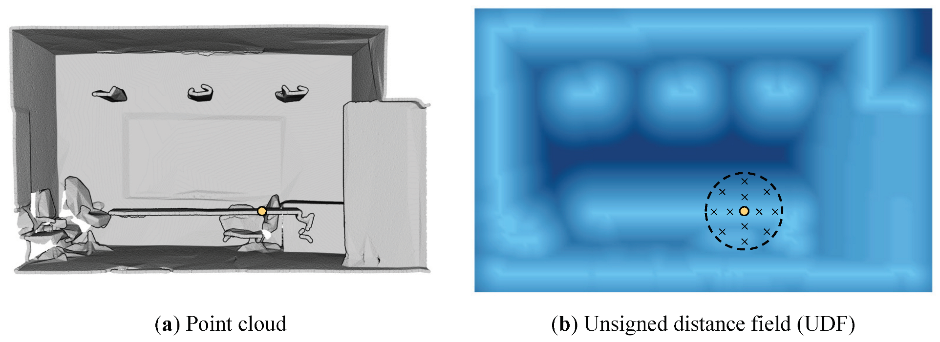
3.1. Implicit Feature Encoding

We choose UDF among shape implicit representations since it can represent both closed objects and open scenes. Given the point cloud of a shape P = { p | p R 3 } , its UDF is a continuous function d P ( · ) that specifies the magnitude of a position x R 3 within the field as the shortest distance between x and P , i.e.,
d P ( x ) = min p P x p .
This function returns a zero value when x is a point of P , and d P ( x ) = 0 defines the point cloud P itself.
To obtain pointwise discrete implicit features from the continuous distance field given by Equation (1), we sample the distance function around each point and concatenate their values in a specific order (see Figure 2). In our implementation, we construct a sample sphere S = { x i , 1 i M } with M positions distributed evenly inside a sphere centered at the origin and with a given radius r. When computing the implicit features of a query point q , S is first placed on q by aligning the center of S with q : S q = { x i + q , 1 i M } . Next, S q is transformed to its canonical pose considering the local geometry of q , which is used to achieve rotation invariance of the computed features and will be detailed in Section 3.2. Finally, the distance field values of the M sampled positions are concatenated sequentially (in the same order as their sampled positions) to form the M-dimensional implicit feature vector for q . For simplicity, we use one identical sample sphere for the entire dataset. This way, the spatial relationships of the sampled positions remain consistent for every point in different point clouds within the dataset, which ensures that the resulting implicit features can be compared to differentiate different objects.
A straightforward way to compute an element of a distance field, i.e., the shortest distance between a given position x and a point cloud P , is to first calculate distances from x to all points in P and then find the minimum one. Despite the simplicity of this brute-force algorithm, it can lead to prohibitively long times when processing large point clouds. For efficiency, we cast the calculation of distance field elements as the nearest neighbor search problem. By building a kd-tree from P , we retrieve the nearest point of x to obtain its respective distance value. We normalize each shortest distance value to the unit scale by dividing it by the radius of the sample sphere r. The process of our implicit feature encoding is summarized in Algorithm 1.
Algorithm 1 Implicit feature encoding
Input: a point cloud P R N × 3 and a sample sphere S R M × 3 with a radius r
Output: an augmented point cloud P R N × ( 3 + M )
  1: Initialization: build a kd-tree from P
  2: for each p P  do
  3:  place S on p
  4:  transform S to its canonical pose S can considering the local geometry of p
  5:  for each x S can  do
  6:   calculate the shortest distance d P ( x ) using the kd-tree
  7:   concatenate the normalized distance d P ( x ) / r to p
  8:  end for
  9: end for

3.2. Transformation Invariance

We expect the encoded implicit features to remain consistent concerning transformations, i.e., translating, scaling, or rotating a point cloud should not influence the calculated features.
Translation and scale invariance. Translation and scale invariance are relatively easy to achieve. On the one hand, our encoded implicit features are already invariant to translations because the positions are sampled from the UDF for each point. On the other hand, we eliminate scaling effects for synthetic datasets by fitting point cloud instances with different scales into a unit sphere before implicit feature encoding. For real-world datasets, we can ignore the scaling issue on practical grounds. Point clouds in a real-world dataset do not change in scale because the entire dataset is typically collected using a single instrument (e.g., a depth camera or a LiDAR scanner).
Rotation invariance. To achieve rotation invariance, we propose to transform each sample sphere S q to its canonical pose based on the local geometry of the query point q . First, we construct a spherical neighborhood P q by searching points within the radius r from q . P q is zero-centered by subtracting q from every point in P q . Then, we calculate the intrinsic orthogonal bases, namely the three principal axes, of P q via principal component analysis (PCA) [50,51]. We implement PCA by performing singular value decomposition (SVD) given its high numerical accuracy and stability [51]. Specifically, P q , when viewed as an N q × 3 matrix (where N q is the number of points in P q ), can be decomposed into two orthogonal matrices U and V , and a diagonal matrix Σ , i.e.,
P q = U Σ V ,
where the columns of V are the three principal axes v 1 , v 2 , v 3 . To eliminate the possible sign ambiguity, we orient every principal axis towards a predefined anchor point p a :
v i = v i , v i · ( q p a ) < 0 v i , otherwise .
In our experiments, the anchor point is chosen as the farthest point from q in its spherical neighborhood P q . Finally, we obtain the canonical sample sphere S can by aligning the three principal axes of the initial sphere with the world coordinate system:
S can = S q · V .
S can is a rotation-equivariant representation, and it remains relatively stationary to the point cloud under external rotations (please refer to Appendix A for a proof). This ensures that encoded implicit features are invariant to rotations.
In real-world datasets, the Z axis of a point cloud typically points vertically upward. We can exploit this a priori information by performing 2D PCA using only the x and y coordinates of the points. In this case, the anchor point can be defined as the farthest neighboring point from the query point in the vertical direction, e.g., the local highest point.
The presented local canonicalization differs significantly from conventional canonicalization methods in two respects.
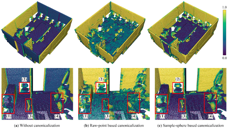
  • We calculate the canonical pose based on local neighborhoods rather than an entire point cloud instance. Therefore, our approach can be applied to not individual objects but also large scenes containing multiple objects.
  • We transform sample spheres instead of raw points, which guarantees the continuity of the encoded features (see Figure 3c). On the contrary, converting raw points of local neighborhoods to their canonical poses will destroy the original geometry of shapes and thus lead to inconsistent features (see Figure 3b). Moreover, canonicalizing sample spheres allows us to employ the pre-built kd-tree structure to accelerate feature encoding.

4. Results and Evaluation

4.1. Implementation Details

We have implemented our implicit feature encoding algorithm in C++ based on the Point Cloud Library [52]. For efficiency, we have parallelized implicit feature encoding using OpenMP [53]. All experiments were carried out on a single NVIDIA GeForce RTX 2080 Ti graphics card.

4.2. Experiment Setup

The goal of our experiments is to validate if the proposed point representation can improve the performance of a range of existing 3D deep neural networks rather than achieve state-of-the-art performance on individual datasets. For this purpose, we have evaluated our method on two classic point cloud analysis tasks: individual object classification and scene-level semantic segmentation. The former aims to determine a category label for a point cloud of a given object as a whole, while the latter intends to assign a category label to each point in a point cloud of a given scene.
First, we employed PointNet [7], Point Structuring Net [22], and CurveNet [21] as our backbones to classify point clouds of individual objects from the ModelNet dataset [23]. PointNet is the foremost deep network that can consume 3D points directly. Point Structuring Net and CurveNet are up-to-date methods that improve point cloud geometry learning through novel feature aggregation paradigms. We compared the results with and without our implicit features in terms of overall accuracy (OA) and mean class accuracy (mAcc).
We then validated our approach for the 3D semantic segmentation task. On the one hand, we tested our method on the large-scale indoor scene dataset S3DIS [24] using three baseline methods: PointNet [7], Superpoint Graph [19], and RandLA-Net [20]. The last two networks are state-of-the-art architectures designed for processing large-scale point clouds. On the other hand, we examined our method on the urban-scale outdoor scene dataset SensatUrban [25] based on the RandLA-Net backbone [20]. Following previous studies, we evaluated network performance quantitatively using three evaluation metrics, i.e., OA, mAcc, and mean intersection over union (mIoU). We also reported per-class IoU for better interpretation of the results.
Table 1 and Table 2 summarize the experimental setting and evaluation metrics, respectively. To ensure a fair comparison, we have trained two models for each baseline network, one with and the other one without our implicit feature encoding. The hyperparameters and training setups of all baselines remain the same as suggested in their original papers (or code repositories [54]). For the RandLA-Net backbone, we have increased the dimension of its first fully connected layer and corresponding decoder layer from 8 to 32 to preserve more information from our implicit features.

4.3. 3D Classification of Individual Objects

We first evaluated our method for the 3D object classification task by comparing the performance of the PointNet [7], Point Structuring Net [22], and CurveNet [21] backbones with and without our implicit features on the ModelNet dataset [23]. ModelNet is the most widely used benchmark dataset for 3D point cloud classification. It contains 40 common classes of CAD models with a total of 12,311 individual objects, of which 9843 and 2468 form the training and test sets, respectively. Each point cloud instance consists of 10,000 points sampled from its synthetic CAD model. Objects of the same category are pre-aligned to a common upward and forward orientation. Before feeding each point cloud into the networks, we uniformly sampled 1024 points from its original point cloud and normalized the points into a unit sphere.
We have conducted two types of experiments to evaluate the effectiveness of our implicit feature encoding and local canonicalization.
  • Pre-aligned. We utilized the a priori orientation information provided by the data in the same way as in the previous studies [7,8,15,21,22,41,55], and we directly calculated implicit features from the data without canonicalizing sample spheres.
  • Randomly rotated. We intentionally introduced random 3D rotation to all point clouds in both training and test sets, and we apply our local canonicalization before implicit feature encoding. We used 3D random rotations as data augmentation for the training.
Table 3 reports the classification results. Our method consistently improved the performance of all three baselines in both types of experiments. When classifying pre-aligned objects, we have observed performance boosts of 2.5% in OA and 2.6% in mAcc for PointNet, 1.1% in OA and 1.3% in mAcc for Point Structuring Net, and 1.0% in OA and 0.3% in mAcc for CurveNet, respectively. The performance gains are more significant for the classification of objects with random poses, with increases of 15.3% in OA and 14.8% in mAcc for PointNet, 6.4% in OA and 8.3% in mAcc for Point Structuring Net, and 2.3% in both OA and mAcc for CurveNet, respectively. It is also worth noting that classifying objects in arbitrary poses is more challenging, resulting in performance drops for both baseline and our method. Nevertheless, our method effectively enriches point cloud data with canonical geometric information, and it thus substantially improved the robustness of the baseline network against unknown rotations. Compared to NerualEmbedding [34] that exploits implicit representations for 3D object analysis, our method plugging the most basic PointNet backbone yielded more accurate predictions with an approximate improvement of 1.1% in terms of both OA and mAcc.

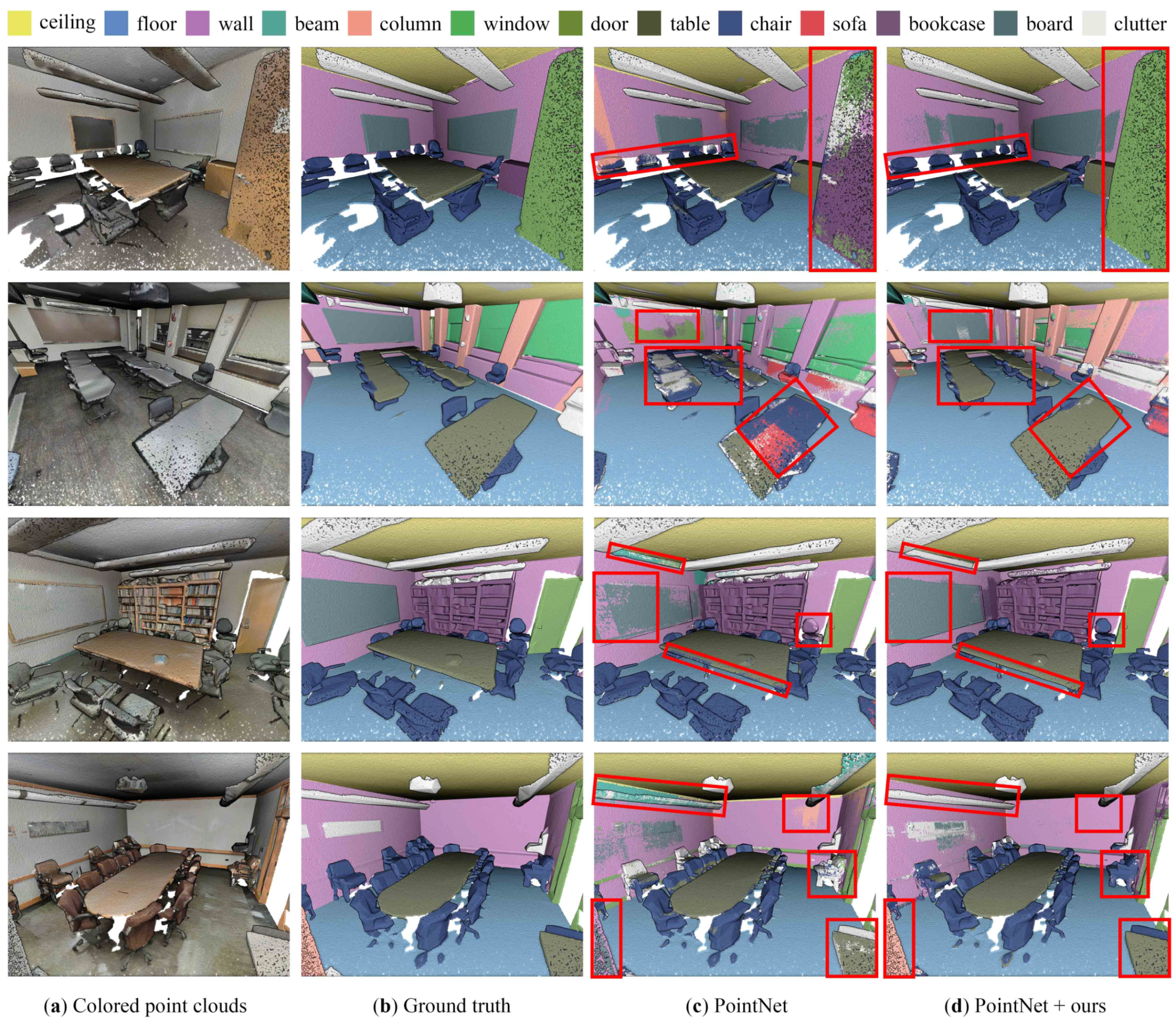
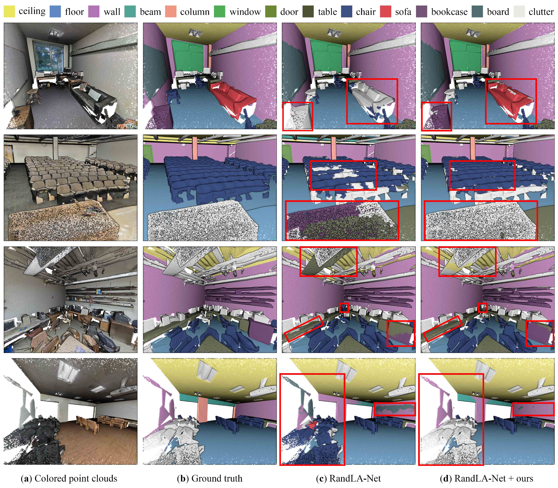
4.4. 3D Semantic Segmentation of Indoor Scenes

Next, we evaluated our method for the 3D semantic segmentation task using three baseline methods, namely PointNet [7], SuperPoint Graph [19], and RandLA-Net [20], on the S3DIS dataset [24]. S3DIS is a large-scale 3D indoor scene dataset that contains six areas with 272 rooms covering approximately 6000 m 2 . The entire dataset comprises 273 million points captured by a Matterport scanner. Each point has its x y z coordinates and several attributes, i.e., an R G B color and a label representing one of the 13 semantic categories. Following the previous studies [7,9,11,15,16,19,20], we have conducted both one-fold experiments using Area 5 as the test set and six-fold cross-validation experiments.
Figure 4 and Figure 5 visualize some qualitative results, from which we can see that our method has successfully corrected the erroneous predictions made by the baseline methods for quite a few categories, such as chair, door, desk, column, sofa, bookcase, wall, and clutter. Besides, the regions of tables in the second row of Figure 4 and those of chairs and clutter in the second row of Figure 5 exemplify better continuity of the predictions generated using our method. Note that Figure 4 and Figure 5 only illustrate the major differences between our predictions and those of the baselines. Due to the random nature of neural networks, our method does not always outperform baselines at every single point prediction. For an accurate comparison, we perform a detailed quantitative analysis.
Table 4 presents the quantitative results of all methods tested on Area 5. We can see that our approach has improved the performance of all three baseline methods in terms of all three evaluation metrics. As PointNet is not designed to capture local information, our implicit features complement this deficiency and thus have enhanced its performance significantly, with increases of 4.1%, 10.5%, and 9.7% in OA, mAcc, and mIoU, respectively. Though SuperPoint Graph and RandLA-Net both exploit local aggregation operations, using our implicit features can still improve their performance. Specifically, using our implicit features has increased the OA, mAcc, and mIoU by 2.1%, 1.3%, and 3.3% for the SuperPoint Graph baseline, and by 1.2%, 3.1%, and 2.7% for the RandLA-Net baseline, respectively. In terms of per-class IoU, enhancing PointNet, SuperPoint Graph, and RandLA-Net by our implicit features has enabled more accurate predictions in 12, 10, and 9 (out of 13) categories, respectively.
Figure 4. Qualitative comparison between the semantic segmentation results of PointNet [7] and ours on the S3DIS dataset [24]. The red rectangles highlight the major differences between the results of PointNet and ours.
Remotesensing 15 00061 g004
Figure 5. Qualitative comparison between the semantic segmentation results of RandLA-Net [20] and ours on the S3DIS dataset [24]. The red rectangles highlight the major differences between the results of RandLA-Net and ours.
Remotesensing 15 00061 g005
Table 5 provides a quantitative comparison of all methods using six-fold cross-validation. Similarly, by feeding our implicit features, all three baseline methods have been improved in all three evaluation metrics. Specific improvements regarding OA, mAcc, and mIoU are 5.2%, 11.0%, and 10.8% for PointNet, 1.4%, 1.7%, and 1.9% for SuperPoint Graph, and 0.5%, 0.7%, and 1.3% for RandLA-Net, respectively. Using our implicit feature encoding, PointNet predicted more accurately in all 13 categories, while SuperPoint Graph and RandLA-Net improved in 10 (out of the 13) categories.

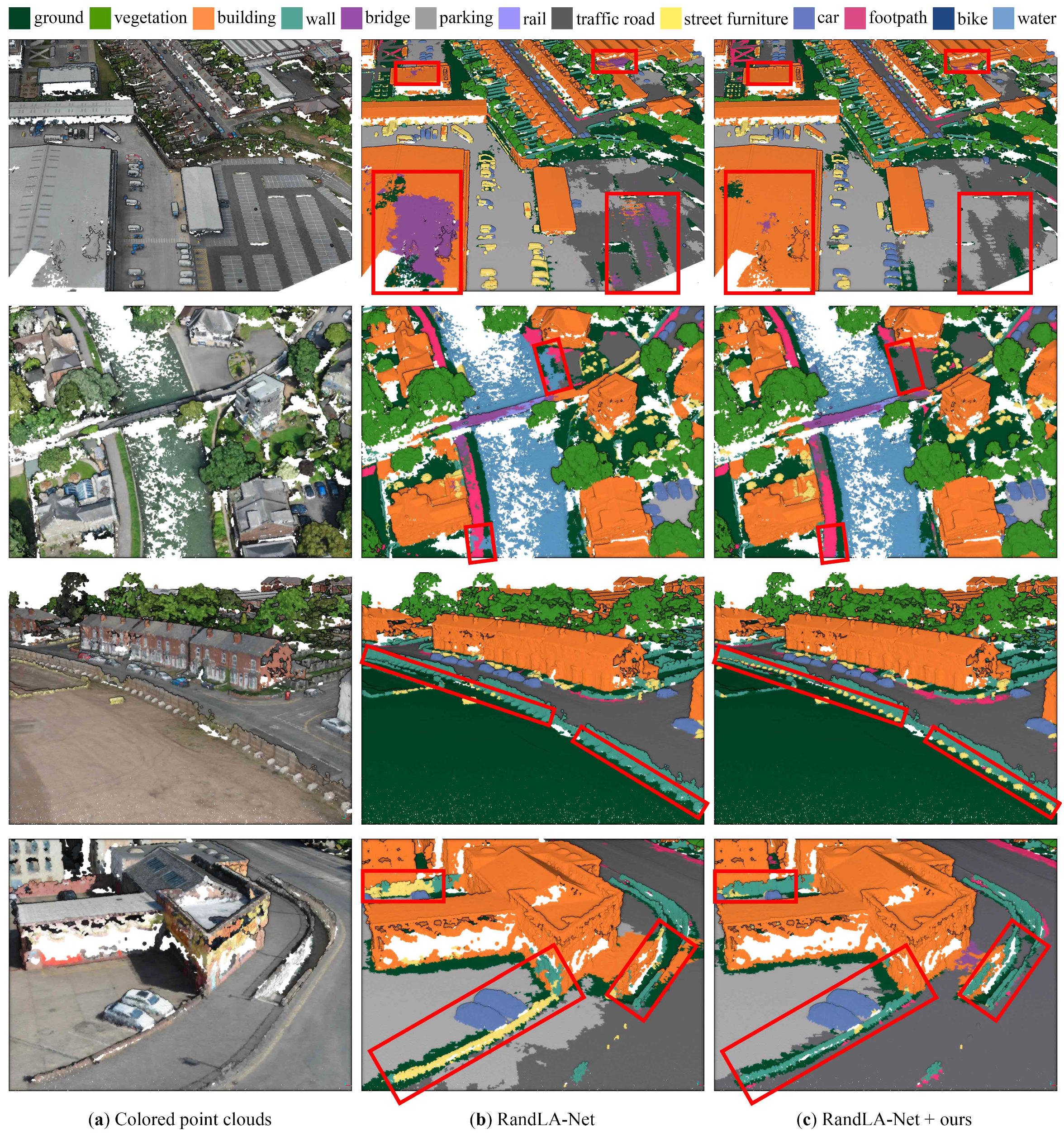
4.5. 3D Semantic Segmentation of Outdoor Scenes

For the 3D semantic segmentation task, we further evaluated our approach on the outdoor scenes from the SensatUrban dataset [25]. SensatUrban covers a total area of 7.6 km 2 across Birmingham, Cambridge, and York. It consists of 37 training blocks and 6 test blocks, totaling approximately 2.8 billion points. Each point has seven dimensions (i.e., x y z coordinates, R G B color, and a label with one of 13 semantic categories). Compared to the indoor dataset S3DIS [24], SensatUrban has urban-scale spatial coverage, a greater number of points, a severer imbalance between categories, and a larger number of missing regions, posing more challenges for semantic segmentation tasks. Because of the large-scale coverage, we used RandLA-Net as our backbone architecture.
Figure 6 visualizes some segmentation results (randomly chosen) of the test set. Due to the unavailable ground-truth labels for the test set, we visually inspected and compared the results by referring to the original-colored point clouds (see Figure 6a). To understand the effect of our implicit features, we manually marked the areas where our predictions differed from those of the baseline method. From these visual results, we can observe that the rich local geometric information encoded by our implicit features enables segmentation at a finer granularity. For example, in the first row of Figure 6, our method substantially reduced the misclassification of points from the ground and roofs as bridges. In the second row of Figure 6, some water segments have been misclassified by the baseline method, while introducing our implicit features has greatly reduced the errors and resulted in more accurate and continuous boundaries between the categories of ground and water. In the third and fourth rows of Figure 6, the walls and street furniture are better separated.
We report the quantitative evaluation on the SensatUrban dataset in Table 6, from which we can see that our segmentation results are superior to those produced by the baseline in 9 out of the 13 categories, leading to a total performance gain of 2.1% in mIoU. There are particularly considerable improvements in IoU for the categories of walls, bridges, and rails, with an increase of 7.1%, 23.1%, and 4.4%, respectively. These improvements are consistent and meanwhile explain the superior quality of our visual results demonstrated in Figure 6.
Figure 6. Visual comparison of semantic segmentation results on the SensatUrban dataset [25]. The red rectangles highlight the major differences in the results between the baseline method and ours.
Remotesensing 15 00061 g006

5. Discussion

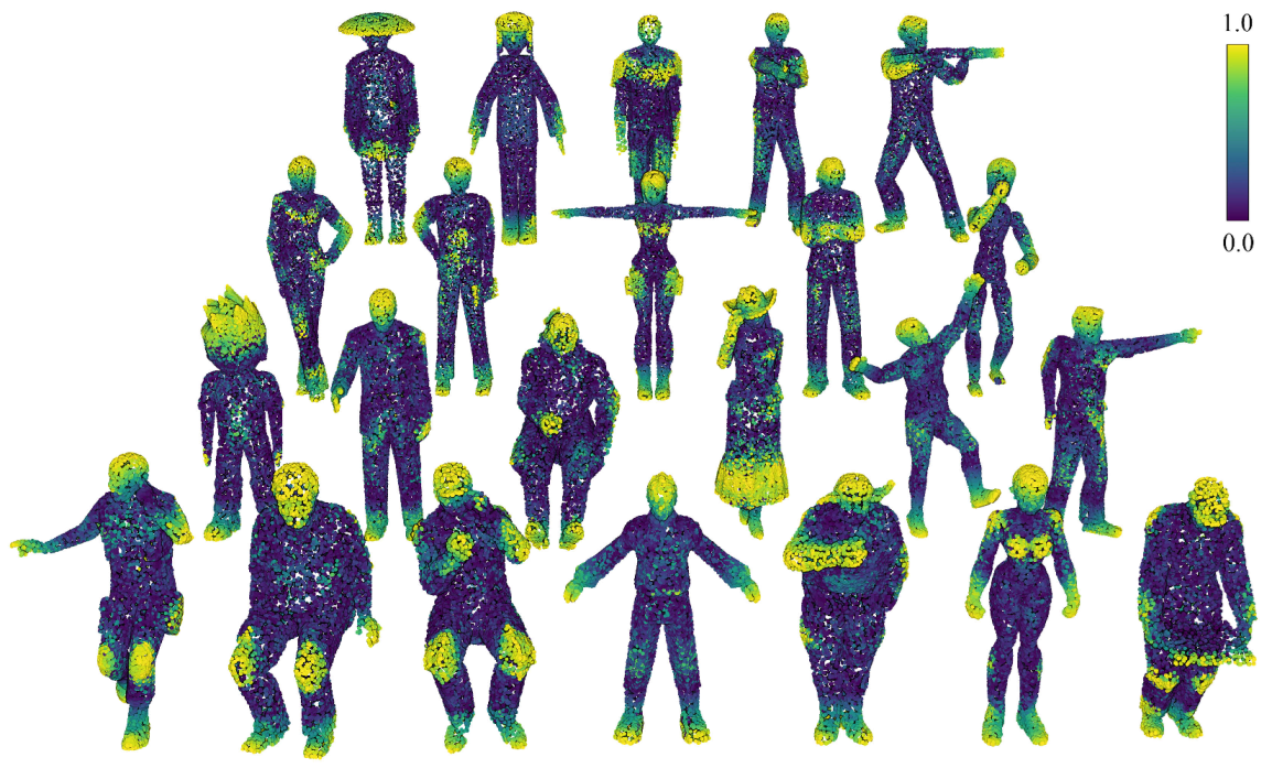
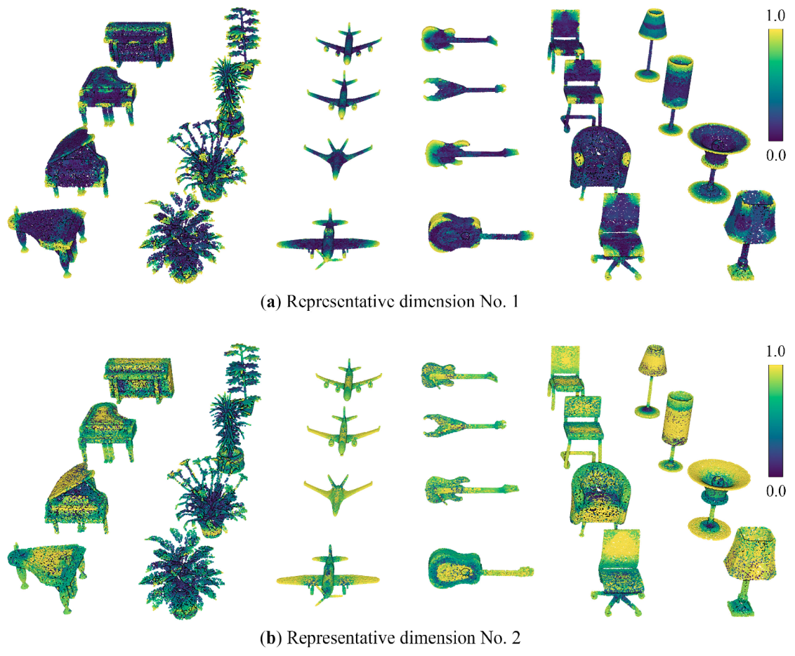
5.1. Feature Visualization
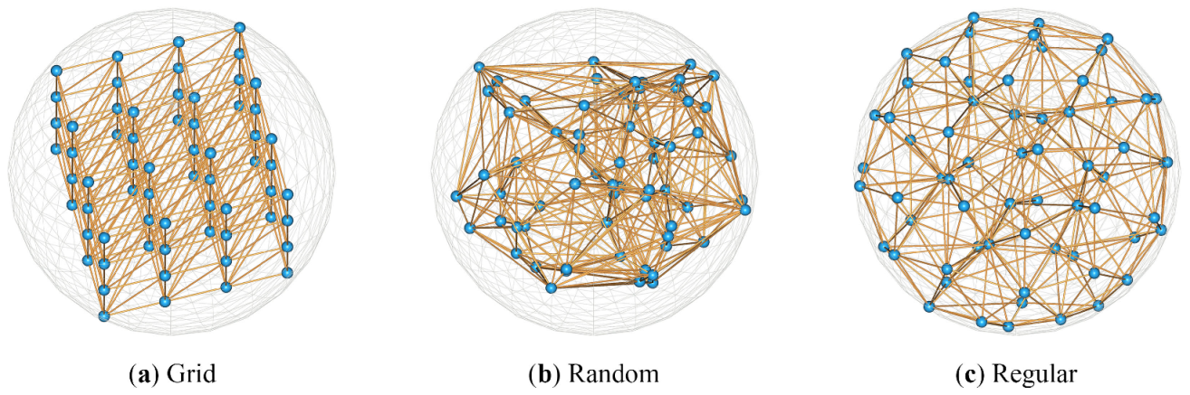
In Section 4, we have demonstrated the effectiveness of our implicit features in both classification and segmentation tasks. In this section, we visualize a few representative dimensions of our implicit features to better understand their effect. Figure 7 shows one (manually chosen) dimension of the implicit features of different persons from the ModelNet dataset [23]. Despite the non-rigid transformations between the persons, this dimension of implicit features captures the same prominent body parts (e.g., head, hands, feet, knees, chest, etc.) highlighted by the brighter color.
To understand how the implicit features distinguish object classes, we visualize in Figure 8 two different dimensions of implicit features for six categories of objects from the ModelNet dataset. From these visualizations, it is interesting that the two dimensions of features capture corners and planar structures, respectively. Besides, the same dimension of the features highlights similar patterns across objects from the same category, and it differentiates objects of different classes.

5.2. Parameters

Our method involves several parameters related to the sample spheres, including the radius of spheres and the number and distribution of the sample positions. The radius of the sample spheres specifies the scale of the local region on which the implicit features are defined, so it is the scale of the locally encoded geometric information. The value of the radius depends on both the point density and the nature of tasks and thus varies across datasets. For the semantic segmentation task, we empirically set the radius to five times the average point density. For the object classification task, as the network treats an entire point cloud instance as a whole, we found that it was beneficial to encode shape information on a relatively larger scale. Specifically, we empirically set the radius to 35 cm for ModelNet [23], 15 cm for S3DIS [24], and 1 m for SensatUrban [25] in our experiments. The number of sample positions determines the dimensionality of our implicit features, and the distribution of sample positions defines the relative spatial relationship among feature dimensions. Figure 9 illustrates three different distributions of sample positions: grid, random, and regular. In Table 7, we report the impact of different parameter settings on the performance of classifying randomly rotated ModelNet objects using the PointNet backbone [7]. For all experiments in this work, we empirically chose 32 regularly distributed sample positions.

5.3. Efficiency

The proposed implicit features encoding does not involve additional networks or training, and they can be efficiently computed from the point clouds. Table 8 reports the running times of implicit feature embedding for the three test datasets. On average, it runs at approximately 290,000 points/s.
In our experiments, we have also observed that involving the proposed implicit feature encoder enables faster convergence of the baseline backbones. To demonstrate this effect, we have trained more epochs for PointNet models both with and without the implicit feature encoder in the task of classifying randomly rotated ModelNet objects. Curves of the training loss and evaluation accuracy of the two models are plotted in Figure 10. The large gap between the corresponding curves indicates that incorporating our implicit features improved the network performance in terms throughout the entire training process. More significantly, our training curves are steeper and converge faster than the corresponding curves of the baseline method. Specifically, the baseline method only shows signs of convergence after Epoch 250, whereas ours starts to converge at Epoch 125. It indicates that our implicit feature encoding transforms point clouds into easier-to-learn representations, thereby increasing the training efficiency.
Table 8. Running times of the proposed implicit feature encoding. The SuperPoint Graph [19] and RandLA-Net [20] backbones use voxel-based downsampling as a pre-processing step, so we calculated implicit features on the downsampled point clouds. As the PointNet backbone [7] does not follow such a procedure, we calculated implicit features on the original input point clouds. #Files and #Points denote the number of files and points, respectively.
Dataset#FilesDownsampled#PointsRunning Times
ModelNet [23]12,311 objects-123,110,0008.7 min
S3DIS [24]272 rooms-273,546,48723.8 min
4 cm18,610,64258 s
SensatUrban [25]43 blocks20 cm220,671,92912.6 min

5.4. Comparison with Point Convolution

Our implicit feature encoding shares the spirit of point convolution methods that exploit local geometric information. Specifically, our method samples values from implicit fields that convey the local geometry of shapes, whereas the point convolution methods strive to enlarge the receptive fields of neurons. We have incorporated our implicit features into the state-of-the-art point convolution method KPConv [15] and tested it in the semantic segmentation task on S3DIS (Area 5). The results are reported in Table 9, from which our implicit features slightly degrade the performance of KPConv. We believe this is due to that the local information captured by point convolution largely overlaps with but is superior to ours. However, it is worth noting that KPConv has high memory and computational requirements, and thus it cannot scale up to large scenes directly. In contrast, our implicit feature encoding is simple, efficient, and can be integrated into network architectures that can directly process point clouds of large-scale scenes, improving both effectiveness and efficiency.

6. Conclusions

We have presented implicit feature encoding, which parameterizes unsigned distance fields into compact point-wise implicit features. Our idea is to transform a point cloud into an easier-to-learn representation by enriching it with local geometric information. We have also introduced a novel local canonicalization approach that ensures the encoded implicit features are transformation-invariant. Our implicit feature encoding is efficient and training-free, which is suitable for both classification of individual objects and the semantic segmentation of large-scale scenes. Extensive experiments on various datasets and baseline architectures have demonstrated the effectiveness of the proposed implicit features.
Our current implementation adopts traditional distance fields that are data-driven and can only represent single-point cloud instances. By contrast, neural distance representations learn to summarize the information of an entire category of point cloud instances, resulting in more powerful descriptiveness and superior robustness against imperfections in the data. In future work, we plan to explore joint implicit feature learning and point cloud classification/segmentation using a multi-task learning framework.

Author Contributions

Z.Y. performed the study, implemented the algorithms, and drafted the original manuscript. Q.Y. and J.S. provided constructive comments and suggestions. L.N. proposed this topic, provided daily supervision, and revised the paper with Z.Y. All authors have read and agreed to the published version of the manuscript.

Funding

Zexin Yang was supported by the China Scholarship Council and International Exchange Program for Graduate Students, Tongji University. Qin Ye was supported by the National Natural Science Foundation of China (No. 41771480).

Data Availability Statement

The source code of our method is publicly available at https://github.com/zexinyang/ImplicitFeatureEncoding, accessed on 23 November 2022. All three datasets used in this study are publicly available. Please refer to ModelNet at https://modelnet.cs.princeton.edu, accessed on 28 July 2022, S3DIS at http://buildingparser.stanford.edu/dataset.html, accessed on 1 March 2022, and SensatUrban at https://github.com/QingyongHu/SensatUrban, accessed on 17 May 2022.

Acknowledgments

We would like to thank Xufei Wang for proofreading the manuscript.

Conflicts of Interest

The authors declare no conflict of interest.

Abbreviations

The following abbreviations are used in this manuscript:
LiDARLight Detection And Ranging
UDFUnsigned Distance Field
CNNConvolutional Neural Network
PCAPrincipal Component Analysis
SVDSingular Value Decomposition
CADComputer-Aided Design

Appendix A

Here we prove that our canonical sample sphere S can is rotation-equivariant w.r.t. its local neighborhood P q .
Proof. 
By applying a random rotation R S O ( 3 ) on P q , its rotated version P q can be obtained as
P q = P q · R .
Similarly to Equations (2) and (4), the SVD of P q can be derived as
P q = P q · R = ( U Σ V ) · R = U Σ ( V R ) = U Σ ( R V ) ,
where the three columns of R V become the axes of the canonical coordinate system. Thus, the canonical sphere S can for P q can be computed as
S can = S q · ( R V ) = ( S q V ) · R = S can · R .
According to Equations (A2) and (A3), we can obtain
S can P q = S can R P q R = S can P q ,
showing that the external rotation matrix R does not affect the relative spatial relationship between a canonical sample sphere and its local neighborhood. □

References

  1. Huang, J.; Stoter, J.; Peters, R.; Nan, L. City3D: Large-Scale Building Reconstruction from Airborne LiDAR Point Clouds. Remote Sens. 2022, 14, 2254. [Google Scholar] [CrossRef]
  2. Peters, R.; Dukai, B.; Vitalis, S.; van Liempt, J.; Stoter, J. Automated 3D reconstruction of LoD2 and LoD1 models for all 10 million buildings of the Netherlands. Photogramm. Eng. Remote Sens. 2022, 88, 165–170. [Google Scholar] [CrossRef]
  3. Luo, L.; Wang, X.; Guo, H.; Lasaponara, R.; Zong, X.; Masini, N.; Wang, G.; Shi, P.; Khatteli, H.; Chen, F.; et al. Airborne and spaceborne remote sensing for archaeological and cultural heritage applications: A review of the century (1907–2017). Remote Sens. Environ. 2019, 232, 111280. [Google Scholar] [CrossRef]
  4. Li, Y.; Ma, L.; Zhong, Z.; Liu, F.; Chapman, M.A.; Cao, D.; Li, J. Deep learning for lidar point clouds in autonomous driving: A review. IEEE Trans. Neural Netw. Learn. Syst. 2020, 32, 3412–3432. [Google Scholar] [CrossRef]
  5. Yousif, K.; Bab-Hadiashar, A.; Hoseinnezhad, R. An overview to visual odometry and visual SLAM: Applications to mobile robotics. Intell. Ind. Syst. 2015, 1, 289–311. [Google Scholar] [CrossRef]
  6. Guo, Y.; Wang, H.; Hu, Q.; Liu, H.; Liu, L.; Bennamoun, M. Deep learning for 3d point clouds: A survey. IEEE Trans. Pattern Anal. Mach. Intell. 2020, 43, 4338–4364. [Google Scholar] [CrossRef]
  7. Qi, C.R.; Su, H.; Mo, K.; Guibas, L.J. Pointnet: Deep learning on point sets for 3d classification and segmentation. In Proceedings of the IEEE Conference on Computer Vision and Pattern Recognition, Honolulu, HI, USA, 21–26 July 2017; pp. 652–660. [Google Scholar]
  8. Qi, C.R.; Yi, L.; Su, H.; Guibas, L.J. Pointnet++: Deep hierarchical feature learning on point sets in a metric space. Adv. Neural Inf. Process. Syst. 2017, 30, 5099–5108. [Google Scholar]
  9. Zhao, H.; Jiang, L.; Fu, C.W.; Jia, J. Pointweb: Enhancing local neighborhood features for point cloud processing. In Proceedings of the IEEE/CVF Conference on Computer Vision and Pattern Recognition, Long Beach, CA, USA, 15–20 June 2019; pp. 5565–5573. [Google Scholar]
  10. Jiang, M.; Wu, Y.; Zhao, T.; Zhao, Z.; Lu, C. Pointsift: A sift-like network module for 3d point cloud semantic segmentation. arXiv 2018, arXiv:1807.00652. [Google Scholar]
  11. Engelmann, F.; Kontogianni, T.; Schult, J.; Leibe, B. Know what your neighbors do: 3D semantic segmentation of point clouds. In Proceedings of the European Conference on Computer Vision (ECCV) Workshops, Munich, Germany, 8–14 September 2018. [Google Scholar]
  12. Hua, B.S.; Tran, M.K.; Yeung, S.K. Pointwise convolutional neural networks. In Proceedings of the IEEE Conference on Computer Vision and Pattern Recognition, Salt Lake City, UT, USA, 18–22 June 2018; pp. 984–993. [Google Scholar]
  13. Wang, S.; Suo, S.; Ma, W.C.; Pokrovsky, A.; Urtasun, R. Deep parametric continuous convolutional neural networks. In Proceedings of the IEEE Conference on Computer Vision and Pattern Recognition, Salt Lake City, UT, USA, 18–23 June 2018; pp. 2589–2597. [Google Scholar]
  14. Engelmann, F.; Kontogianni, T.; Leibe, B. Dilated point convolutions: On the receptive field of point convolutions. arXiv 2019, arXiv:1907.12046. [Google Scholar]
  15. Thomas, H.; Qi, C.R.; Deschaud, J.E.; Marcotegui, B.; Goulette, F.; Guibas, L.J. Kpconv: Flexible and deformable convolution for point clouds. In Proceedings of the IEEE/CVF International Conference on Computer Vision, Seoul, Republic of Korea, 27 October–2 November 2019; pp. 6411–6420. [Google Scholar]
  16. Yang, J.; Zhang, Q.; Ni, B.; Li, L.; Liu, J.; Zhou, M.; Tian, Q. Modeling point clouds with self-attention and gumbel subset sampling. In Proceedings of the IEEE/CVF Conference On Computer Vision and Pattern Recognition, Long Beach, CA, USA, 15–20 June 2019; pp. 3323–3332. [Google Scholar]
  17. Chen, L.Z.; Li, X.Y.; Fan, D.P.; Wang, K.; Lu, S.P.; Cheng, M.M. LSANet: Feature learning on point sets by local spatial aware layer. arXiv 2019, arXiv:1905.05442. [Google Scholar]
  18. Zhao, C.; Zhou, W.; Lu, L.; Zhao, Q. Pooling scores of neighboring points for improved 3D point cloud segmentation. In Proceedings of the 2019 IEEE International Conference on Image Processing (ICIP), Taipei, Taiwan, 22–25 September 2019; pp. 1475–1479. [Google Scholar]
  19. Landrieu, L.; Simonovsky, M. Large-scale point cloud semantic segmentation with superpoint graphs. In Proceedings of the IEEE Conference on Computer Vision and Pattern Recognition, Salt Lake City, UT, USA, 18–23 June 2018; pp. 4558–4567. [Google Scholar]
  20. Hu, Q.; Yang, B.; Xie, L.; Rosa, S.; Guo, Y.; Wang, Z.; Trigoni, N.; Markham, A. Learning semantic segmentation of large-scale point clouds with random sampling. IEEE Trans. Pattern Anal. Mach. Intell. 2021, 44, 8338–8354. [Google Scholar] [CrossRef] [PubMed]
  21. Xiang, T.; Zhang, C.; Song, Y.; Yu, J.; Cai, W. Walk in the cloud: Learning curves for point clouds shape analysis. In Proceedings of the IEEE/CVF International Conference on Computer Vision, Montreal, QC, Canada, 11–17 October 2021; pp. 915–924. [Google Scholar]
  22. Li, L.; He, L.; Gao, J.; Han, X. PSNet: Fast Data Structuring for Hierarchical Deep Learning on Point Cloud. IEEE Trans. Circuits Syst. Video Technol. 2022, 32, 6835–6849. [Google Scholar] [CrossRef]
  23. Wu, Z.; Song, S.; Khosla, A.; Yu, F.; Zhang, L.; Tang, X.; Xiao, J. 3d shapenets: A deep representation for volumetric shapes. In Proceedings of the IEEE Conference on Computer Vision and Pattern Recognition, Boston, MA, USA, 7–12 June 2015; pp. 1912–1920. [Google Scholar]
  24. Armeni, I.; Sax, S.; Zamir, A.R.; Savarese, S. Joint 2d-3d-semantic data for indoor scene understanding. arXiv 2017, arXiv:1702.01105. [Google Scholar]
  25. Hu, Q.; Yang, B.; Khalid, S.; Xiao, W.; Trigoni, N.; Markham, A. Sensaturban: Learning semantics from urban-scale photogrammetric point clouds. Int. J. Comput. Vis. 2022, 130, 316–343. [Google Scholar] [CrossRef]
  26. Michalkiewicz, M.; Pontes, J.K.; Jack, D.; Baktashmotlagh, M.; Eriksson, A. Implicit surface representations as layers in neural networks. In Proceedings of the IEEE/CVF International Conference on Computer Vision, Seoul, Republic of Korea, 27 October–2 November 2019; pp. 4743–4752. [Google Scholar]
  27. Ran, H.; Liu, J.; Wang, C. Surface Representation for Point Clouds. In Proceedings of the IEEE/CVF Conference on Computer Vision and Pattern Recognition, New Orleans, LA, USA, 19–20 June 2022; pp. 18942–18952. [Google Scholar]
  28. Tretschk, E.; Tewari, A.; Golyanik, V.; Zollhöfer, M.; Stoll, C.; Theobalt, C. Patchnets: Patch-based generalizable deep implicit 3d shape representations. In Proceedings of the European Conference on Computer Vision, Glasgow, UK, 23–28 August 2020; Springer: Berlin/Heidelberg, Germany, 2020; pp. 293–309. [Google Scholar]
  29. Michalkiewicz, M.; Pontes, J.K.; Jack, D.; Baktashmotlagh, M.; Eriksson, A. Deep level sets: Implicit surface representations for 3d shape inference. arXiv 2019, arXiv:1901.06802. [Google Scholar]
  30. Park, J.J.; Florence, P.; Straub, J.; Newcombe, R.; Lovegrove, S. Deepsdf: Learning continuous signed distance functions for shape representation. In Proceedings of the IEEE/CVF Conference on Computer Vision and Pattern Recognition, Long Beach, CA, USA, 15–20 June 2019; pp. 165–174. [Google Scholar]
  31. Peng, S.; Niemeyer, M.; Mescheder, L.; Pollefeys, M.; Geiger, A. Convolutional occupancy networks. In Proceedings of the European Conference on Computer Vision, Glasgow, UK, 23–28 August 2020; Springer: Berlin/Heidelberg, Germany, 2020; pp. 523–540. [Google Scholar]
  32. Jiang, C.; Sud, A.; Makadia, A.; Huang, J.; Nießner, M.; Funkhouser, T. Local implicit grid representations for 3d scenes. In Proceedings of the IEEE/CVF Conference on Computer Vision and Pattern Recognition, Seattle, WA, USA, 13–19 June 2020; pp. 6001–6010. [Google Scholar]
  33. Juhl, K.A.; Morales, X.; Backer, O.D.; Camara, O.; Paulsen, R.R. Implicit neural distance representation for unsupervised and supervised classification of complex anatomies. In Proceedings of the International Conference on Medical Image Computing and Computer-Assisted Intervention, Strasbourg, France, 27 September–1 October 2021; Springer: Berlin/Heidelberg, Germany, 2021; pp. 405–415. [Google Scholar]
  34. Fujiwara, K.; Hashimoto, T. Neural implicit embedding for point cloud analysis. In Proceedings of the IEEE/CVF Conference on Computer Vision and Pattern Recognition, Seattle, WA, USA, 13–19 June 2020; pp. 11734–11743. [Google Scholar]
  35. Lawin, F.J.; Danelljan, M.; Tosteberg, P.; Bhat, G.; Khan, F.S.; Felsberg, M. Deep projective 3D semantic segmentation. In Proceedings of the International Conference on Computer Analysis of Images and Patterns, Ystad, Sweden, 22–24 August 2017; Springer: Berlin/Heidelberg, Germany, 2017; pp. 95–107. [Google Scholar]
  36. Boulch, A.; Le Saux, B.; Audebert, N. Unstructured point cloud semantic labeling using deep segmentation networks. 3dor@ Eurograph. 2017, 3, 1–8. [Google Scholar]
  37. Su, H.; Maji, S.; Kalogerakis, E.; Learned-Miller, E. Multi-view convolutional neural networks for 3d shape recognition. In Proceedings of the IEEE International Conference on Computer Vision, Santiago, Chile, 7–13 December 2015; pp. 945–953. [Google Scholar]
  38. Boulch, A.; Guerry, J.; Le Saux, B.; Audebert, N. SnapNet: 3D point cloud semantic labeling with 2D deep segmentation networks. Comput. Graph. 2018, 71, 189–198. [Google Scholar] [CrossRef]
  39. Maturana, D.; Scherer, S. Voxnet: A 3d convolutional neural network for real-time object recognition. In Proceedings of the 2015 IEEE/RSJ International Conference on Intelligent Robots and Systems (IROS), Hamburg, Germany, 28 September–3 October 2015; pp. 922–928. [Google Scholar]
  40. Meng, H.Y.; Gao, L.; Lai, Y.K.; Manocha, D. Vv-net: Voxel vae net with group convolutions for point cloud segmentation. In Proceedings of the IEEE/CVF International Conference on Computer Vision, Seoul, Republic of Korea, 27 October–2 November 2019; pp. 8500–8508. [Google Scholar]
  41. Wang, Y.; Sun, Y.; Liu, Z.; Sarma, S.E.; Bronstein, M.M.; Solomon, J.M. Dynamic graph cnn for learning on point clouds. ACM Trans. Graph. 2019, 38, 1–12. [Google Scholar] [CrossRef] [Green Version]
  42. Li, F.; Fujiwara, K.; Okura, F.; Matsushita, Y. A closer look at rotation-invariant deep point cloud analysis. In Proceedings of the IEEE/CVF International Conference on Computer Vision, Montreal, BC, Canada, 11–17 October 2021; pp. 16218–16227. [Google Scholar]
  43. Li, X.; Li, R.; Chen, G.; Fu, C.W.; Cohen-Or, D.; Heng, P.A. A rotation-invariant framework for deep point cloud analysis. IEEE Trans. Vis. Comput. Graph. 2021, 28, 4503–4514. [Google Scholar] [CrossRef]
  44. Deng, H.; Birdal, T.; Ilic, S. Ppf-foldnet: Unsupervised learning of rotation invariant 3d local descriptors. In Proceedings of the European Conference on Computer Vision (ECCV), Munich, Germany, 8–14 September 2018; pp. 602–618. [Google Scholar]
  45. Zhang, Z.; Hua, B.S.; Rosen, D.W.; Yeung, S.K. Rotation invariant convolutions for 3d point clouds deep learning. In Proceedings of the 2019 International Conference on 3d Vision (3DV), Québec City, QC, Canada, 16–19 September 2019; pp. 204–213. [Google Scholar]
  46. Chen, C.; Li, G.; Xu, R.; Chen, T.; Wang, M.; Lin, L. Clusternet: Deep hierarchical cluster network with rigorously rotation-invariant representation for point cloud analysis. In Proceedings of the IEEE/CVF Conference on Computer Vision and Pattern Recognition, Long Beach, CA, USA, 15–20 June 2019; pp. 4994–5002. [Google Scholar]
  47. Yu, R.; Wei, X.; Tombari, F.; Sun, J. Deep positional and relational feature learning for rotation-invariant point cloud analysis. In Proceedings of the European Conference on Computer Vision, Glasgow, UK, 23–28 August 2020; Springer: Berlin/Heidelberg, Germany, 2020; pp. 217–233. [Google Scholar]
  48. Kim, S.; Park, J.; Han, B. Rotation-invariant local-to-global representation learning for 3d point cloud. Adv. Neural Inf. Process. Syst. 2020, 33, 8174–8185. [Google Scholar]
  49. Xiao, Z.; Lin, H.; Li, R.; Geng, L.; Chao, H.; Ding, S. Endowing deep 3d models with rotation invariance based on principal component analysis. In Proceedings of the 2020 IEEE International Conference on Multimedia and Expo (ICME), London, UK, 6–10 July 2020; pp. 1–6. [Google Scholar]
  50. Shlens, J. A tutorial on principal component analysis. arXiv 2014, arXiv:1404.1100. [Google Scholar]
  51. Abdi, H.; Williams, L.J. Principal component analysis. Wiley Interdiscip. Rev. Comput. Stat. 2010, 2, 433–459. [Google Scholar] [CrossRef]
  52. Rusu, R.B.; Cousins, S. 3d is here: Point cloud library (pcl). In Proceedings of the 2011 IEEE International Conference on Robotics and Automation, Shanghai, China, 9–13 May 2011; pp. 1–4. [Google Scholar]
  53. Dagum, L.; Menon, R. OpenMP: An industry standard API for shared-memory programming. IEEE Comput. Sci. Eng. 1998, 5, 46–55. [Google Scholar] [CrossRef]
  54. Yan, X. Pointnet/Pointnet++ Pytorch. 2019. Available online: https://github.com/yanx27/Pointnet_Pointnet2_pytorch (accessed on 8 February 2022).
  55. Li, Y.; Bu, R.; Sun, M.; Wu, W.; Di, X.; Chen, B. Pointcnn: Convolution on x-transformed points. Adv. Neural Inf. Process. Syst. 2018, 31, 820–830. [Google Scholar]
Figure 1. The proposed implicit feature encoding. Given a point cloud as input, its unsigned distance field (UDF) is sampled as pointwise canonical feature vectors and concatenated after the point coordinates, forming a more expressive point cloud representation. The UDF is color-coded from bright to dark in ascending order of the distance values of the points.
Remotesensing 15 00061 g001
Figure 2. Implementation of implicit feature encoding. For a query point q (yellow dot), the sample sphere is aligned with q and projected to its canonical pose. q ’s implicit feature vector is then obtained by sequentially concatenating the UDF values of each sample position (black cross). The UDF is color-coded from bright to dark in ascending order of the distance values of the points.
Remotesensing 15 00061 g002
Figure 3. The impact of canonicalization on the encoded implicit features. Here we visualize the same randomly chosen dimension of the encoded implicit features under three different canonicalization settings. The four red rectangles (i.e., 1–4) in subfigures highlight noticeable differences among implicit features under different settings. (a) Without canonicalization, walls and chairs with the same orientation (e.g., 1 and 2) share similar implicit features, whereas those with varying orientations (e.g., 1 and 4) show different implicit features. (b) By transforming raw points of local neighborhoods to their canonical poses, the encoded implicit features are inconsistent. (c) By transforming sample spheres to their canonical poses, the implicit features become consistent and invariant to rotations (i.e., each object class has similar implicit features).
Remotesensing 15 00061 g003
Figure 7. Visualization of one (manually chosen) dimension of the implicit features for the person category from the ModelNet dataset [23]. With this dimension of implicit features, the same prominent body parts are highlighted by the brighter color regardless of their postures.
Remotesensing 15 00061 g007
Figure 8. Visualization of two (manually chosen) dimensions of the implicit features for six categories of point clouds from the ModelNet dataset [23].
Remotesensing 15 00061 g008
Figure 9. Illustration of three different distributions of 64 sample positions (blue dots). The orange edges in this figure are derived from the Delaunay triangulation of the sample positions, which are intended for visualization purposes.
Remotesensing 15 00061 g009
Figure 10. Training curves for 3D object classification using the PointNet backbone [7] on randomly rotated objects from the ModelNet dataset [23].
Remotesensing 15 00061 g010
Table 1. Experimental setting. PN: PointNet [7]. PSN: Point Structuring Net [22]. CN: CurveNet [21]. SPG: SuperPoint Graph [19]. RLN: RandLA-Net [20]. #Classes and #Points denote the number of classes and points, respectively.
TaskDatasetBaseline(s)
NameScenarioData SourceArea#Classes#PointsRGB
ClassificationModelNet [23]ObjectsSynthetic-4012 MNoPN, PSN, CN
SegmentationS3DIS [24]Indoor scenesMatterport6.0 × 10 3 m 2 13273 MYesPN, SPG, RLN
SensatUrban [25]Urban scenesUAV photogrammetry7.6 × 10 6 m 2 132847 MYesRLN
Table 2. Evaluation metrics. C denotes the number of classes. TP, TN, FP, and FN are the true positive, true negative, false positive, and false negative, separately.
MetricFormulaTask (s)
Overall Accuracy OA = TP + TN TP + TN + FP + FN Classification & Segmentation
Mean Class Accuracy mAcc = 1 C i = 1 C TP i TP i + FN i Classification & Segmentation
Mean Intersection Over Union mIoU = 1 C i = 1 C TP i TP i + FP i + FN i Segmentation
Table 3. Object classification results (%) on the ModelNet dataset [23].
MethodPre-AlignedRandomly Rotated
OAmAccOAmAcc
PointNet [7]90.887.871.067.7
PointNet [7] + ours93.390.486.382.5
Point Structuring Net [22]92.389.281.976.0
Point Structuring Net [22] + ours93.490.588.384.3
CurveNet [21]93.190.487.483.1
CurveNet [21] + ours94.190.789.785.4
NeuralEmbedding [34]92.289.3--
Table 4. Quantitative comparison between the semantic segmentation results of PointNet [7], SuperPoint Graph [19], RandLA-Net [20], and ours on Area 5 of the S3DIS dataset [24].
MethodOAmAccmIoUCeil.FloorWallBeamCol.Wind.DoorTableChairSofaBook.BoardClut.
PointNet [7]77.951.340.987.397.869.00.55.935.94.457.442.18.048.538.336.0
PointNet [7] + ours81.961.850.692.498.072.20.022.144.028.965.264.229.457.642.440.9
SPG [19]86.466.558.089.496.978.10.042.848.961.675.484.752.669.82.152.2
SPG [19] + ours88.567.861.393.096.879.20.034.452.265.977.887.372.973.17.756.2
RandLA-Net [20]87.170.562.591.597.680.30.022.760.237.178.787.069.970.766.051.5
RandLA-Net [20] + ours88.373.665.293.196.982.30.032.059.553.076.588.470.872.468.254.8
Table 5. Quantitative comparison between the semantic segmentation results of PointNet [7], SuperPoint Graph [19], RandLA-Net [20], and ours on the S3DIS dataset [24] using six-fold cross validation.
MethodOAmAccmIoUCeil.FloorWallBeamCol.Wind.DoorTableChairSofaBook.BoardClut.
PointNet [7]78.561.248.388.493.869.329.620.244.950.052.843.515.541.837.441.2
PointNet [7] + ours83.772.259.192.394.375.538.740.246.461.361.364.742.451.948.351.0
SPG [19]85.573.062.189.995.176.462.847.155.368.469.273.545.963.28.752.9
SPG [19] + ours86.974.764.092.095.676.644.550.455.772.568.979.059.863.114.658.9
RandLA-Net [20]88.082.070.093.196.180.662.448.064.469.469.476.460.064.265.960.1
RandLA-Net [20] + ours88.582.771.394.096.481.260.753.463.272.570.977.168.865.162.361.2
Table 6. Quantitative comparison of semantic segmentation results on the SensatUrban dataset [25].
MethodOAmIoUGroundVeg.Build.WallBridgePark.RailTraff.Street.CarFoot.BikeWater
RandLA-Net [20]91.254.283.998.293.954.537.750.311.353.139.379.036.10.067.9
RandLA-Net [20] + ours91.356.384.298.194.661.660.844.215.749.437.279.137.80.168.7
Table 7. The effect of the parameters of sample spheres on the classification of randomly-rotated objects from the ModelNet dataset [23] using the PointNet backbone [7].
ParameterDistributionRadius (cm)Dimension
GridRandomRegular253545163264
OA (%)85.285.586.383.686.385.585.186.386.2
Table 9. Comparison between the results of KPConv [15] and ours in the semantic segmentation task on the S3DIS dataset [24] (Area 5).
MethodmIoUCeil.FloorWallBeamCol.Wind.DoorTableChairSofaBook.BoardClut.
KPConv [15]65.393.397.981.60.018.153.768.781.390.866.074.364.857.9
KPConv [15] + ours65.393.298.080.80.017.554.569.480.891.671.374.260.856.3
Disclaimer/Publisher’s Note: The statements, opinions and data contained in all publications are solely those of the individual author(s) and contributor(s) and not of MDPI and/or the editor(s). MDPI and/or the editor(s) disclaim responsibility for any injury to people or property resulting from any ideas, methods, instructions or products referred to in the content.

