Hyperspectral Feature Selection for SOM Prediction Using Deep Reinforcement Learning and Multiple Subset Evaluation Strategies

Abstract

It has been widely certified that hyperspectral images can be effectively used to monitor soil organic matter (SOM). Though numerous bands reveal more details in spectral features, information redundancy and noise interference also come accordingly. Due to the fact that, nowadays, prevailing dimensionality reduction methods targeted to hyperspectral images fail to make effective band selections, it is hard to capture the spectral features of ground objects quickly and accurately. In this paper, to solve the inefficiency and instability of hyperspectral feature selection, we proposed a feature selection framework named reinforcement learning for feature selection in hyperspectral regression (RLFSR). Specifically, the Markov Decision Process (MDP) was used to simulate the hyperspectral band selection process, and reinforcement learning agents were introduced to improve model performance. Then two spectral feature evaluation methods were introduced to find internal relationships between the hyperspectral features and thus comprehensively evaluate all hyperspectral bands aimed at the soil. The feature selection methods—RLFSR-Net and RLFSR-Cv—were based on pre-trained deep networks and cross-validation, respectively, and achieved excellent results on airborne hyperspectral images from Yitong Manchu Autonomous County in China. The feature subsets achieved the highest accuracy for most inversion models, with inversion R² values of 0.7506 and 0.7518, respectively. The two proposed methods showed slight differences in spectral feature extraction preferences and hyperspectral feature selection flexibilities in deep reinforcement learning. The experiments showed that the proposed RLFSR framework could better capture the spectral characteristics of SOM than the existing methods.

1. Introduction

Soil organic matter (SOM) is an essential component of soil, and monitoring SOM is a crucial element of soil quality assessment [1]. Since the advent of hyperspectral sensors, the acquisition capability of hyperspectral data has been dramatically enhanced, and large-scale and detailed ground observation has become possible, which can provide rich data support for soil environmental quality monitoring [2,3]. As a result, hyperspectral images, with their rich and continuous spectral bands from visible to short-wave infrared, have been widely used in predictions of SOM [4,5,6]. The numerous spectral bands of hyperspectral images provide the possibility of accurate extraction of SOM reflection features, but at the same time, the noise and useless information contained in the data can interfere with SOM prediction. Therefore, it is necessary to reduce the hyperspectral data redundancy when building hyperspectral SOM regression models.

To make full use of the valid information from hyperspectral data, researchers have usually conducted characterization of the raw spectra before building a regression model. Specifically, spectral transformations based on signal processing, such as simple mathematical transformations and frequency domain transformations, are able to detect the changing features that are sensitive to the target variables and can increase the amount of effective information in hyperspectral data. Next, researchers have explored various means of dimensionality reduction concerning the rich spectral information. Feature selection, which can remove redundant information while preserving the physical meaning of the original image spectra, is one of the main methods for the dimensionality reduction of hyperspectral data, which also enhances the interpretation of the subsequent modeling process from a spectral perspective.

Feature selection is the process of selecting a subset of relevant features or candidate features and using evaluation criteria to obtain the optimal subset. Subset generation is mainly accomplished by a heuristic search. There are three main search methods: sequential search, exhaustive search, and random search [7]. The sequential search iteratively adds and removes features to complete the subset generation. Many methods have been proposed based on this idea, such as sequential forward selection (SFS) [8,9,10], sequential backward elimination (SBE) [11,12], and bi-directional selection [13]. Shafiee et al. [14] investigated the performance of support vector regression (SVR) in combination with SFS for grain yield prediction and showed that SVR in combination with SFS is a robust method. The exhaustive search iterates through all the possible feature subsets to generate the best solution. Although it is possible to obtain the best and most stable subset, this usually consumes a lot of computational resources and time. Random search starts with a random feature subset and generates the next subset in the feature space according to the preset strategy. The typical random search algorithms, such as simulated annealing [15], genetic algorithms [16], evolutionary programming [17], and particle swarm optimization [18,19], sacrifice optimality guarantees to quickly finding a relatively good solution [20]. However, due to the random sampling process of the algorithms, there is instability in the search process, and two random search processes can lead to very different results. Meanwhile, it is necessary to evaluate the newly generated feature subset using certain criteria. The optimal subset of features generated from the same data can vary according to the evaluation criteria. Based on the dependence and independence of the algorithms, there are independent criteria and dependent criteria. Independent criteria do not involve any learning algorithm, and they use the underlying characteristics of the training data to evaluate the performance of a subset of features. Many independent criteria have been proposed in the literature, including distance measures [21], information or uncertainty measures [22], probability of error measures [23], dependency measures [24,25], interclass distance measures [26], and consistency measures [27], which are generally very efficient. However, the dependent criteria require a predefined mining algorithm to evaluate the goodness of the feature subset and determine which features are selected. Although dependent criteria usually obtain better performance, they come with a greater computational cost [21,28].

In hyperspectral data processing, various dimensionality reduction methods are widely used. The common feature selection methods include variable importance in the projection (VIP), the successive projections algorithm (SPA), the Pearson product–moment correlation coefficient (PPMCC), competitive adaptive reweighted sampling (CARS), genetic algorithms (GAs), and simulated annealing (SA). Bangelesa et al. [29] applied the VIP and recursive feature selection methods to feature selection in partial least squares (PLS) regression and random forest regression, respectively, and finally determined that the significant wavelengths for SOM prediction were located in the range of 400–700 nm. Song et al. [30] reduced the dimensionality of HJ-1A hyperspectral data with the help of the Pearson’s correlation coefficient and principal component analysis (PCA), and the extracted feature spectra achieved better results on a back-propagation neural network (BPNN) model with double hidden layers. Wei et al. [31] proposed a gradient boosting regression tree (GBRT) hyperspectral inversion algorithm based on Spearman’s rank correlation analysis (SCA) coupled with CARS, which achieved a better inversion effect than the support vector machine and random forest. Kawamura et al. [32] applied a GA to select significant bands in laboratory visible and near-infrared spectroscopy, and found that the GA has the advantage of optimizing the PLS regression bands.

The common methods mentioned above usually employ conventional feature collection and evaluation methods, which are not optimized for hyperspectral data. As a result, the obtained feature subsets cannot guarantee a satisfactory output in the inversion modeling, and the stability of the methods is questionable. Moreover, the above methods are limited by the inefficient search capability, which makes it challenging to extract superior and small-scale feature subsets quickly. In addition to the common feature selection methods already described, deep learning has also been applied to hyperspectral data processing. In the field of hyperspectral feature selection, a novel ternary weight convolution neural network (TWCNN) was proposed, which uses a depth-wise convolutional layer with 1 × 1 filters as the first layer of the network, and can achieve end-to-end feature selection and classification [33]. Lorenzo et al. [34] developed a data-driven hyperspectral band selection algorithm that couples an attention-based convolutional neural network to identify the most information-rich regions in the spectrum. Meanwhile, the framework named integrated learning and feature selection (ILFS) [35] determines the characteristic bands by measuring the contribution of each band to the overall loss of the optimization. This approach is effective for the dimensionality reduction of multispectral and hyperspectral imagery, and can significantly improve the performance in the semantic segmentation task for high-dimensional imagery. Bernal et al. [36] learned a convolutional Siamese network by optimizing the contrast loss, and they performed band selection based on the low-dimensional data embedding generated by the network. However, the deep network-based feature selection techniques require considerable computational resources and have limitations when balancing the accuracy and efficiency of computing the optimal subset.

Deep reinforcement learning (DRL) combines the perceptual capabilities of deep learning with the decision-making capabilities of reinforcement learning in a generalized form. The powerful exploration capabilities of DRL allow us to strike a better balance between finding the optimal subset and conserving computational resources, which allows for better adaptation to different task requirements by adjusting the reward policy. Some researchers have considered the band selection task of hyperspectral imagery as a combinatorial optimization problem of searching for band combinations in discrete space and solving the feature selection problem with the learning ability of DRL. Mou et al. [37] defined the unsupervised band selection problem as a Markov decision process (MDP), and explored the application of DRL in hyperspectral image analysis by using information entropy as the reward function for adding new bands. Feng et al. [38] established a semi-supervised convolutional neural network to evaluate the band selection state, and achieved efficient evaluation of the band state for image classification tasks through limited labeled sample errors and intra-class tightness constraints for unlabeled samples, which was shown to be an effective approach for the publicly available hyperspectral classification datasets.

By designing a reasonable reward policy, DRL can quickly and accurately generate feature subsets that solve the problem of the unstable hyperspectral feature extraction results of the commonly used methods. In addition, in hyperspectral inversion work, we are more interested in features strongly correlated with the inversion parameters. According to the characteristics of the inversion index and the requirements of inversion modeling, DRL can flexibly adjust the optimization strategy to select the spectral features for better SOM prediction. In this paper, we propose a feature selection framework named reinforcement learning for feature selection in hyperspectral regression (RLFSR). By modeling the hyperspectral feature search problem as an MDP, we introduce two spectral feature sampling strategies that use the internal linkage of the hyperspectral features and the accuracy of the hyperspectral inversion as comprehensive evaluation indicators. Specifically, we adopted sample data to pre-train an inverse network and evaluate the feature subsets by inversion accuracy, which was named RLFSR-Net. In contrast, RLFSR-Cv ran cross-validation on the dataset to assess the value of the results. Finally, the advantage actor critic (A2C) algorithm was introduced to optimize the set of features by maximizing the expected cumulative rewards of the MDP.

Our contributions are summarized as follows:

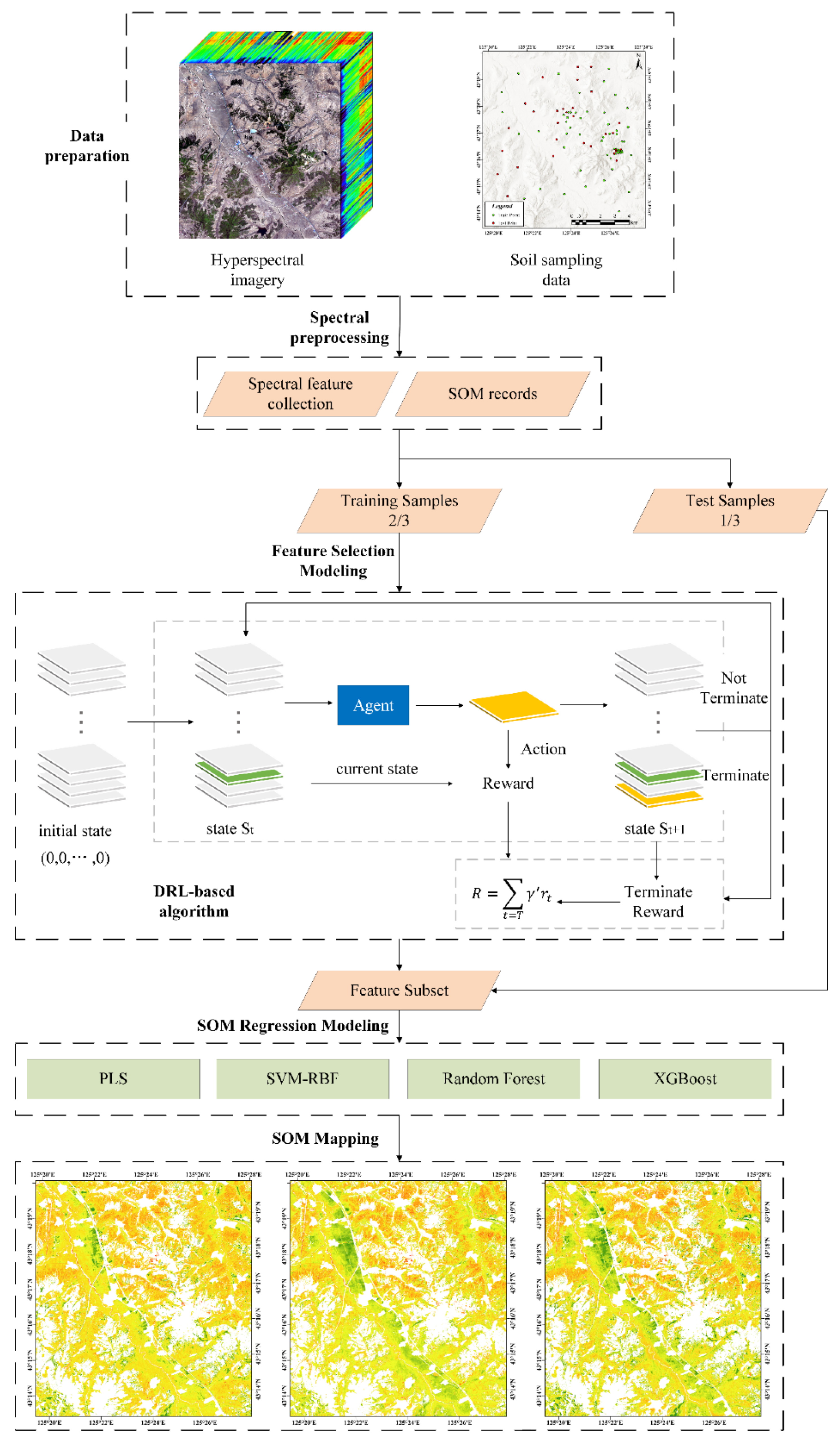
• To achieve efficient and accurate feature selection, a reinforcement learning framework was proposed. A supervised feature selection method was used, which considered the needs of the inversion task. We believe this is the first time reinforcement learning has been introduced into feature selection for a hyperspectral inversion task.
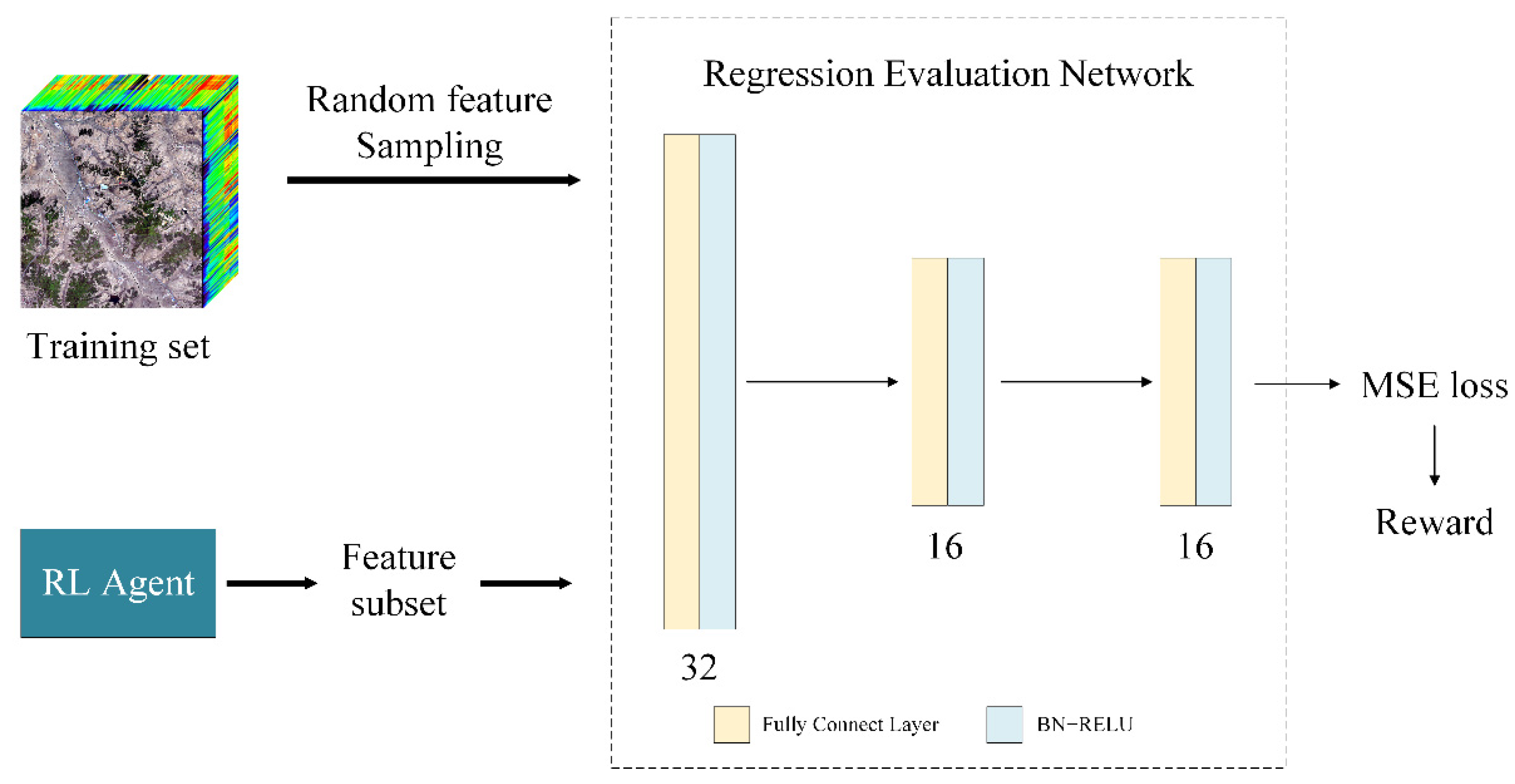
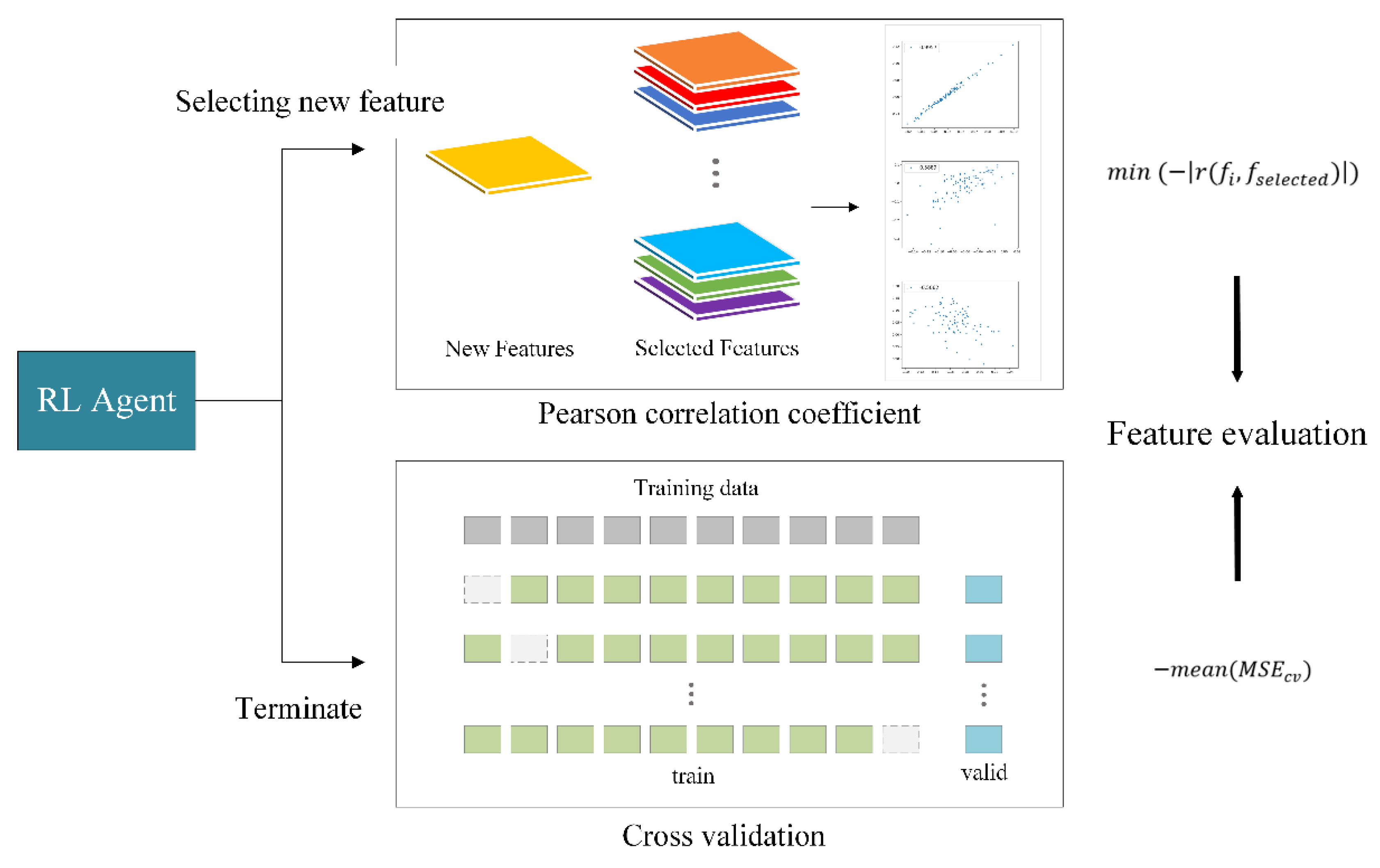
• The spectral feature selection problem was formulated as an MDP. A selection agent was then constructed, and the state of the agent was updated based on the spectral feature selection. To comprehensively evaluate the value of the features selected by the agent, two evaluation strategies were proposed: RLFSR-Net and RLFSR-Cv. With the support of the two strategies, the training of the feature selection model was completed to maximize the cumulative reward.
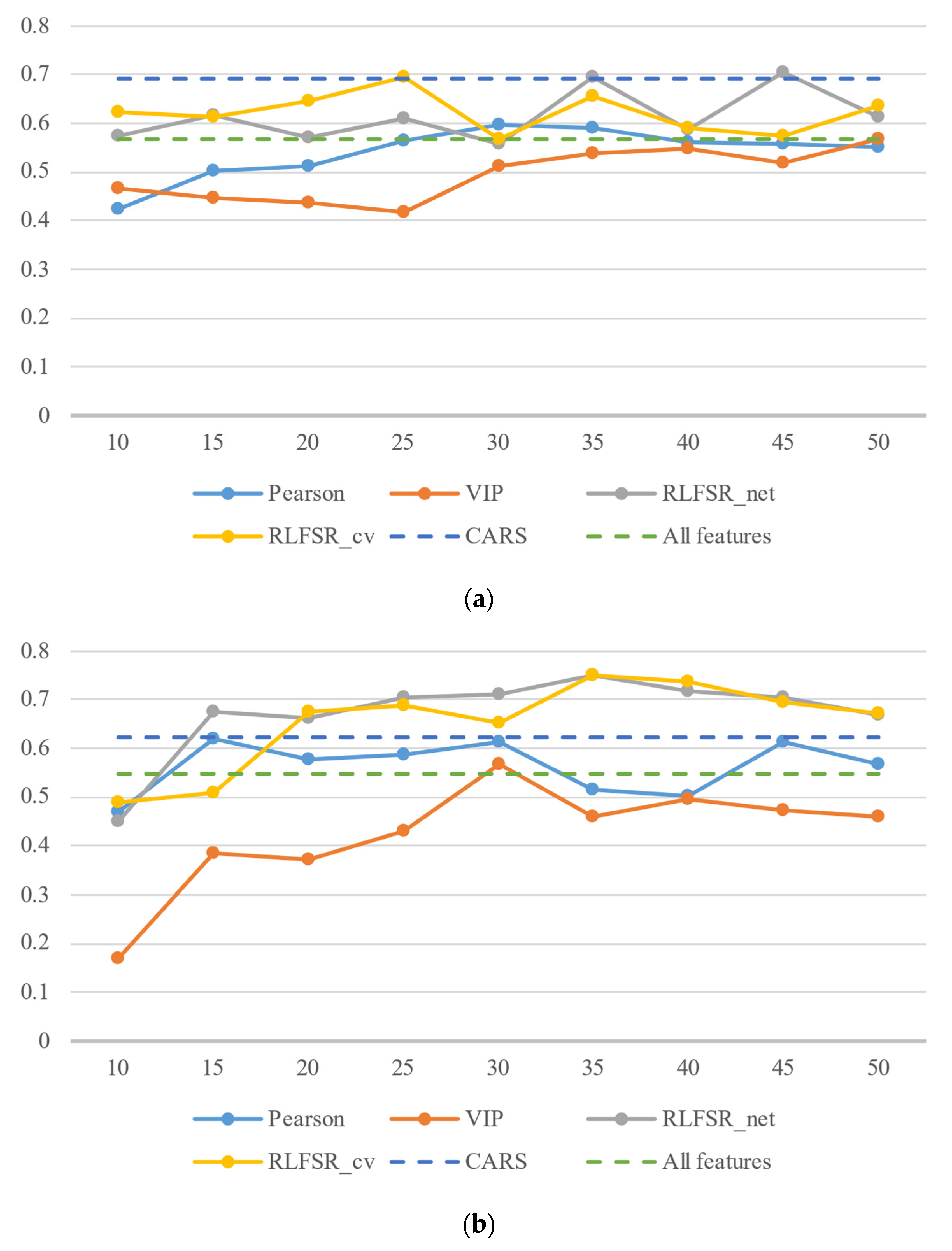
• The feature subsets selected by RLFSR-Net and RLFSR-Cv achieved inversion results that were comparable with those of the XGBoost model, and they outperformed the other data dimensionality reduction methods. As the number of features increased, the inversion accuracy of the feature subset generally improved. However, after reaching a certain number of features, the inversion accuracy decreased instead, due to the increase in noise and invalid information.
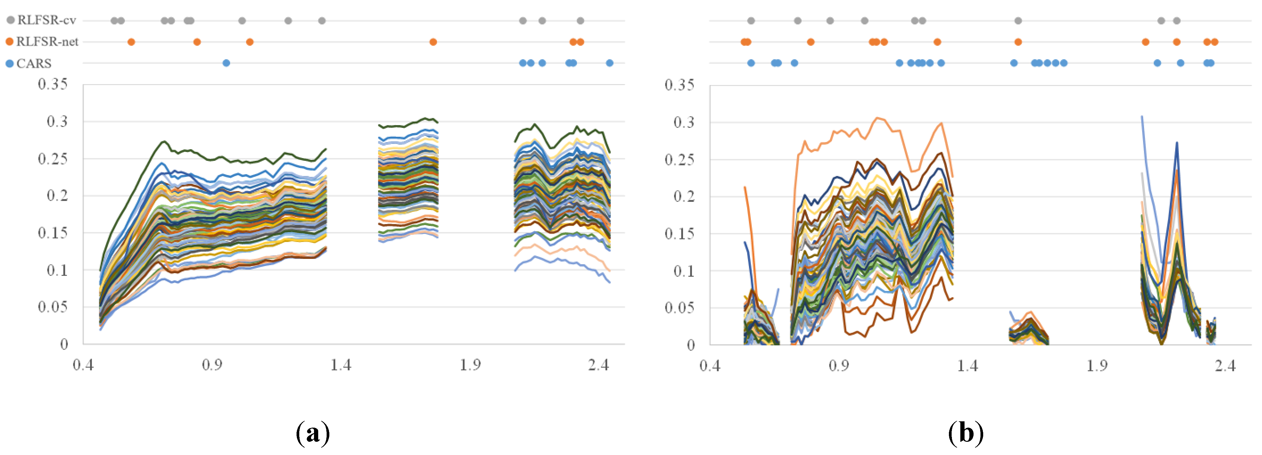
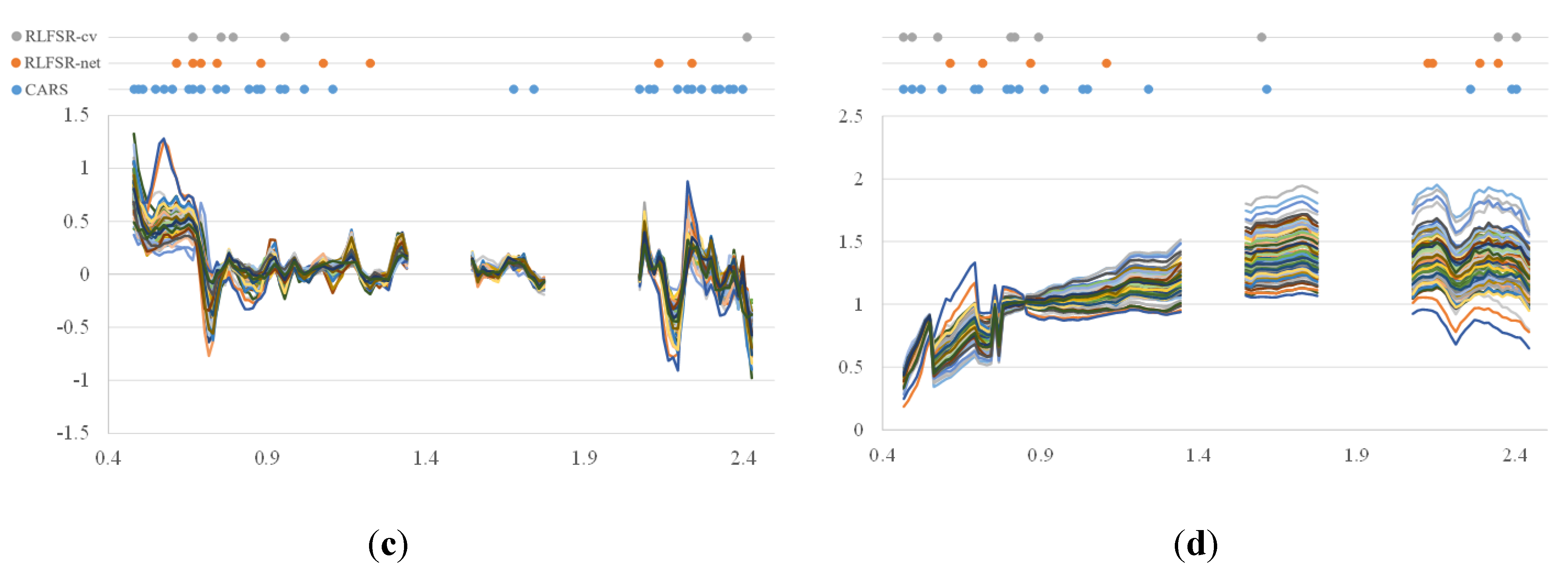
• The spectral features extracted by RLFSR-Net and RLFSR-Cv appeared to be in high agreement with those extracted by CARS, and were concentrated in the visible range and 2.2 μm, which was in line with the experience of SOM inversion. However, the proposed method could extract a more compact subset of features and achieve better inversion results.

The rest of this paper is organized as follows. Section 2 introduces the proposed methods in detail, including the Markov modeling for feature selection and the two feature subset evaluation strategies. In Section 3, we describe the experimental results obtained on airborne hyperspectral data from the Yitong Manchu Autonomous County in China. The discussion is presented in Section 4 to show the effectiveness of the RLFSR. In Section 5, the conclusions of this paper are provided.

2. Methods

The proposed RLFSR framework is displayed in Figure 1. This feature selection framework is designed from a reinforcement learning perspective, and includes the MDP modeling for the feature-selecting agent and the reward function settings. Firstly, the hyperspectral SOM regression dataset was constructed based on airborne hyperspectral images and laboratory chemical observations, and the training set and test set were randomly, divided according to the SOM distribution, with a ratio of 2:1. The training set was then used for the feature selection modeling. With regard to the agent’s MDP modeling, the feature selection status was described in the form of a {0,1} array, where 0 means unselected and 1 means selected. Every time the actions of selecting features were executed, the state and reward were updated for the training of the agent. Two reward strategies—RLFSR-Net and RLFSR-Cv—were then introduced to evaluate the subset of features. RLFSR-Net is based on pretraining an inverse network to obtain the reward function, and RLFSR-Cv evaluates the subset with the help of cross-validation accuracy. Finally, the reinforcement learning agent was trained based on the A2C algorithm, which used an experienced pool for recording the agent behavior. Finally, a subset of features was generated for the training and testing with the help of the trained DRL-based algorithm, and the SOM regression model was built to perform the SOM mapping.

2.1. Feature Selection Modeling

As is shown in Figure 1, a reinforcement learning agent was introduced for the feature selection. It was necessary to formulate the process as an MDP, which allowed the reinforcement learning agent to optimize the feature selection problem. The core elements of the MDP were the state, the action, the Markov transition function, the reward, and the discount factor.

(1) The state $s$: In this feature selection case, the state $s$ records the history of the feature selection. It consists of a set of n-dimensional vectors, which are coded to represent the selection among the n features. The i-th chosen feature among n is denoted as $s_i=1$, while $s_i=0$ means that this feature is not selected for now.

(2) The action $a$: The action of the agent, in this case, includes choosing a feature from the hyperspectral image or stopping. The action is determined by the current state of the agent and constraints. Until the set number of features is reached, the agent will continue the act of selection; otherwise, it will end the work.

(3) The transition function $P$: When an action is performed, the state $s$ transitions from the previous state to a new one. This transformation process is defined as the transition function $P$. The function $P$ is determined by the current state–action pair. For example, the state $s_t$ at time $t$ will convert to a new state $s_{t+1}$ if the action is to choose a new feature. The state $s_t$ will remain the same if the selected feature already exists in $s_t$, and will finally terminate when reaching the preset number of bands.

$$s_{t+1}=\left\{\begin{array}{cc}Terminal& if reaching the preset number\\ s_t& if a_t=select a feature that already exists in s_t\\ s_t+f_i& if a_t=select a new feature\end{array}\right.$$

(1)

(4) The reward $r$: The reward $r_t$ refers to the reward expectation that can be obtained by performing the action $a_t$ in the current state $s_t$ and moving to the next moment. The reward function is the reward gained by leaving the state, not the reward gained by entering the state. In this case, two types of reward functions are modeled— RLFSR-Net and RLFSR-Cv—which evaluate the final feature subset in different ways.

$$r_t=\left\{\begin{array}{cc}Final reward function& if reaching the preset number\\ Penalty factor C& if a_t=select a feature that already exists in s_t\\ Process reward function& if a_t=select a new feature\end{array}\right.$$

(2)

The final reward function and process reward function in the above formula are defined differently in RLFSR-Net and RLFSR-Cv, and they are introduced in Section 2.2 and Section 2.3. The penalty factor C is a constant to suppress repetitive features.

(5) The discount factor $\gamma$: In most Markov reward processes and MDPs, the discount factor $\gamma \in \left[0,1\right]$ is introduced to reduce the uncertainty of the forward earnings, in that immediate rewards can be more beneficial than longer-term ones.

2.2. Feature Evaluation in RLFSR-Net

The current research on feature selection using reinforcement learning frameworks has focused on classification tasks, with unsupervised and semi-supervised methods being primarily used to evaluate the feature subsets. In the inversion task, we are more interested in whether the features are correlated with the inversion parameters, so we designed a supervised evaluation procedure. Inspired by the pre-trained evaluation networks introduced in [38], we built a hyperspectral regression deep neural network (DNN) that was trained by random features extracted from the dataset as the final reward function. In each epoch, some feature dimensions were shut down randomly in the training set to explore the most effective feature combinations. The objective function of the regression part was MSE loss.

As is shown in Figure 2, the framework of RLFSR-Net included three main parts: (1) feature generation; (2) the DNN for inversion; and (3) the reward calculation module. In the part of feature generation, the state of the MDP coded as {0,1} arrays was translated to a subset of the original feature data for reward calculation. A common type of DNN, which is mainly stacked by fully connected layers, was introduced for evaluation. To avoid the gradient disappearance problem and to speed up the training, batch normalization layers were added after the fully connected layers. The coefficient of determination (R²), the mean square error (MSE), and the mean absolute error (MAE) are usually measured in terms of prediction accuracy. Therefore, in the reward calculation module, the MSE of the output of the DNN with respect to the true value was taken as the evaluation index.

It was finally necessary to perform the computation of the reward with the {0,1} array transformed by the feature selection case. Therefore, random {0,1} arrays were generated in the training process, and the corresponding numbered features were selected and fed into the DNN, with MSE as the loss function.

When evaluating feature subsets transformed from the terminal state coded as a {0,1} array, the MSE of the subset of all the hyperspectral training datasets is taken to calculate the final reward. Since it can be expected to obtain a subset of features with higher accuracy, and since the MSE represents the error about the true value, $reward=-MS{E}_{subset}$ was accepted in RLFSR-Net. Thus, the reward function of RLFSR-Net was modified as follows:

$$r_t=\left\{\begin{array}{cc}-MS{E}_{subset}& if reaching the preset number\\ \mathrm{C}& if a_t=select a feature that already exists in s_t\\ 0& if a_t=select a new feature\end{array}\right.$$

(3)

where $MS{E}_{subset}$ represents the MSE of the DNN for inversion, and $\mathrm{C}$ is a constant number to avoid repetitive actions. As it is not necessary to reward or punish the new features, the reward will be 0 when selecting a new feature.

2.3. Feature Evaluation in RLFSR-Cv

The basic idea of cross-validation is to group the original data into a training set and a validation set. The training set is first applied to train the model, and then the validation set is used to test the trained model, which is taken as the performance index for evaluating the model. Cross-validation algorithms perform well in parameter tuning for most models and perform the feature selection task in CARS very well. Consequently, in introducing the idea of cross-validation into the DRL framework, we proposed RLFSR-Cv.

2.3.1. Selecting a New Feature

Since there is a dependency between the soil hyperspectral features, especially in the neighboring bands, the selected new features may not enhance the information of the feature subset, and may cause only a small improvement in model accuracy, which does not meet our goal of feature robustness. To avoid selecting spectral features that were too similar, the reward for selecting a new feature was defined as a negative function:

$${\rho }_{xy}=r\left(X,Y\right)=\frac{\mathrm{Cov}\left(X,Y\right)}{\sqrt{\mathrm{Var}\left[X\right]\mathrm{Var}\left[Y\right]}}$$

(4)

The Pearson’s correlation coefficient, which ranges from −1 to 1, describes the degree of linear correlation between the variables. The correlation coefficient ${\rho }_{xy}$ quantitatively portrays the degree of correlation between X and Y. That is, the larger $\left|{\rho }_{xy}\right|$ is, the greater the correlation. In this case, to suppress the selection of relevant features, the Pearson’s correlation coefficient was computed between the newly selected feature and the features already existing in the subset, and min $-\left|{\rho }_{xy}\right|$ was taken as the reward for selecting the new feature, as is shown in the following equation:

$$Process Reward Function=min\left(-\left|r\left(f_i,f_{selected}\right)\right|\right)$$

(5)

where $f_i$ means the newly chosen feature, and $f_{selected}$ represents the features already existing in the subset.

2.3.2. Termination

When the stopping condition of the MDP was satisfied, meaning that the feature subset reached a preset number, the reward function was calculated by the cross-validation algorithm. In this case, the 10-fold cross-validation method was chosen to evaluate the feature subsets. As is shown in Figure 3, the dataset was divided into ten parts, nine of which were rotated for training and testing the accuracy of the remaining data. After completing all the tests, the opposite of the average MSE of the dataset was presented as the final reward:

$$Final Reward Function=-mean\left(MS{E}_{cv}\right)$$

(6)

Therefore, the reward function of RLFSR-Cv was modified as follows:

$$r_t=\left\{\begin{array}{cc}-mean\left(MS{E}_{cv}\right)& if reaching the preset number\\ \mathrm{C}& if a_t=select a feature that already exists in s_t\\ min\left(-\left|r\left(f_i,f_{selected}\right)\right|\right)& if a_t=select a new feature\end{array}\right.$$

(7)

where $MS{E}_{cv}$ represents the MSEs of the 10-fold cross-validation, $\mathrm{C}$ is a constant number to avoid repetitive actions, and $r\left(f_i,f_{selected}\right)$ refers to the Pearson’s correlation coefficient between the new feature and the previous ones.

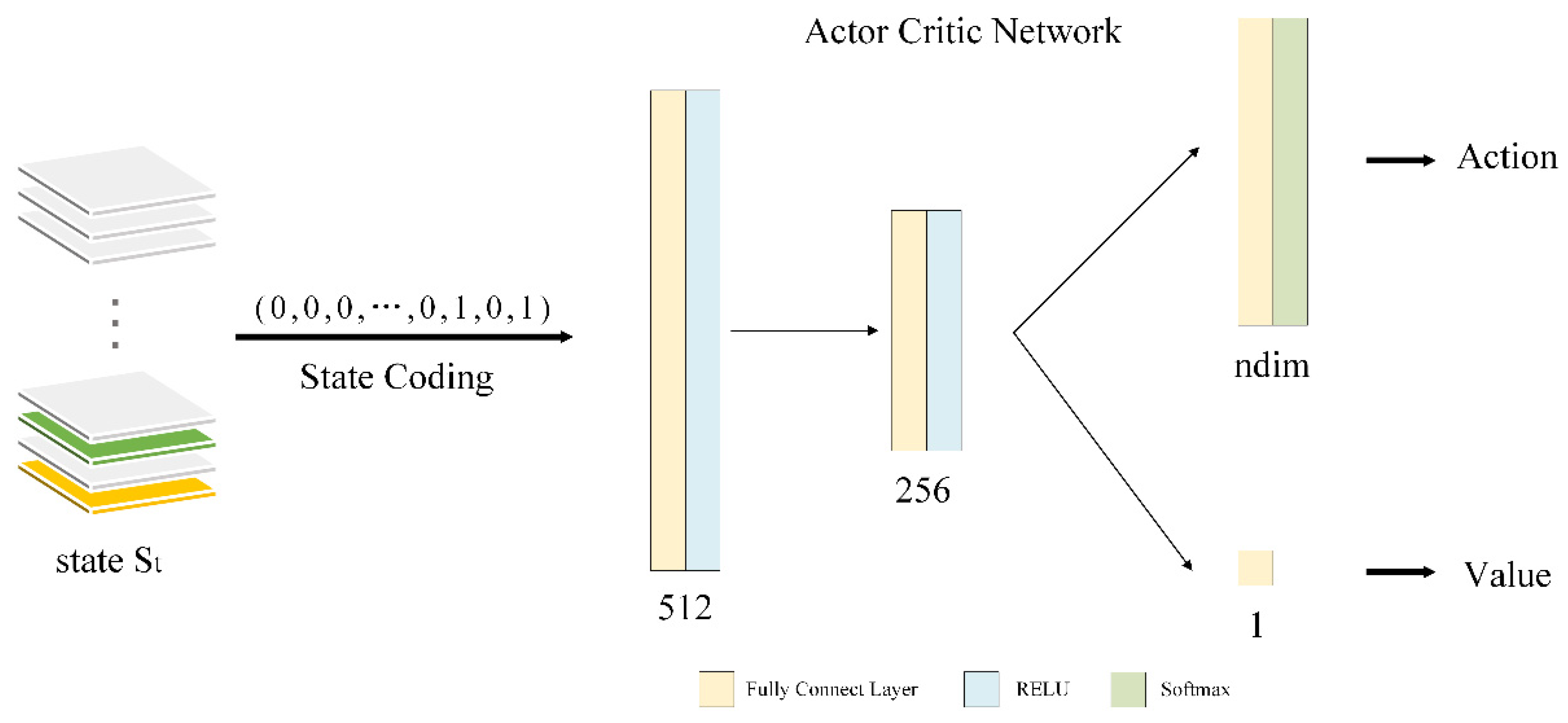
2.4. Deep Reinforcement Learning for the RLFSR Framework

2.4.1. Introduction to Deep Reinforcement Learning

In Section 2.3, we described how the feature selection problem was modeled as the MDP and defined the two forms of reward functions. After completing these tasks, it was now possible to solve the problem by employing a reinforcement learning approach.

In the MDP, it seeks to maximize the long-term return, denoted as $G_t$, which, in the simplest case, is the sum of the returns at each time step:

$$G_t=\sum _{t\ge 0}{\gamma }^t{r}_t=r_t+\gamma r_{t+1}+{\gamma }^2{r}_{t+2}+\cdots +{\gamma }^{T-t}$$

(8)

where $T$ represents the terminal time, and $\gamma$ represents the discount factor that demonstrates a focus on future returns. The larger the value of $\gamma$, the more visionary the discounted payoff is in considering more future returns, while the smaller the value of $\gamma$, the more short-sighted the intelligence is. When $\gamma$ = 0, the intelligence only considers maximizing the current payoff.

In the MDP, the state value function of policy $\pi$, denoted as $v_{\pi }\left(s\right)$, represents the probability expectation value of the gain obtained by the agent from state $s$ by deciding according to policy $\pi$, which is denoted as:

$$v_{\pi }(s)=E_{\pi }[G_t\mid S_t=s]=E_{\pi }[\sum _{k=0}^{\infty }{\gamma }^k{r}_{t+k+1}\mid S_t=s]$$

(9)

Similarly, the action value function of policy $\pi$, denoted as $q_{\pi }\left(s,a\right)$, represents the probability expectation of all the subsequent gains obtained by the agent after taking action starting from state $s$, which is denoted as:

$$q_{\pi }(s,a)=E_{\pi }[G_t\mid S_t=s,A_t=a]=E_{\pi }[\sum _{k=0}^{\infty }{\gamma }^k{r}_{t+k+1}\mid S_t=s,A_t=a]$$

(10)

Since there is a recursive relationship between $v_{\pi }\left(s\right)$ and $q_{\pi }\left(s,a\right)$, based on the Bellman equation, the above equations can be rewritten as follows:

$$v_{\pi }\left(s\right)=E_{\pi }\left[r_{t+1}+\gamma v_{\pi }\left(S_{t+1}\right)\mid S_t=s\right]$$

(11)

$$q_{\pi }\left(s,a\right)=E_{\pi }\left[r_{t+1}+\gamma q_{\pi }\left(S_{t+1},A_{t+1}\right)\mid S_t=s,A_t=a\right]$$

(12)

To solve the reinforcement learning problem, finding an optimal policy that maximizes the reward of the agent in the long-term process is necessary. In the MDP, the optimal policy is denoted as ${\pi }_{*}$, and its state value function $v_{*}$ is the optimal state value function, which is denoted as:

$$v_{*}\left(s\right)=\underset{\pi }{max}{v}_{\pi }\left(s\right)$$

(13)

2.4.2. Training of the A2C Algorithm

Unlike the value-based and policy-based reinforcement learning algorithms, the A2C algorithm is an algorithm that combines value-based and policy-based methods, in that the policy-based actor learns a policy and interacts with the environment, and the value-based critic evaluates the goodness of the policy to guide the next actions.

The actor part is implemented by the policy gradient method, which belongs to the Monte Carlo class of methods. The objective of the policy gradient method is to maximize the reward function by adjusting $\theta$ under policy $\pi$. The objective function is expressed as $J_{\theta }=E_{\pi \sim i}\left[R\left(t\right)\right]$.

The derivation yields the gradient of the objective function as:

$${\nabla }_{\theta }J\left(\theta \right)=E_{{\pi }_{\theta }}\left[{\nabla }_{\theta }\log {\pi }_{\theta }\left(s,a\right)v_t\right]$$

(14)

The A2C algorithm assesses the policy based on an advantage function that reduces the variance without introducing bias, and the advantage function subtracts the estimated value function from a set benchmark, which is generally estimated using the state value function, which is denoted as $A^{{\pi }_{\theta }}\left(s,a\right)=Q\left(s,a\right)-V^{{\pi }_{\theta }}\left(s\right)$.

Therefore, the policy gradient of the A2C algorithm is formalized as follows:

$${\nabla }_{\theta }J\left(\theta \right)=E_{{\pi }_{\theta }}\left[{\nabla }_{\theta }\log {\pi }_{\theta }\left(s,a\right)\left(Q\left(s,a\right)-V^{{\pi }_{\theta }}\left(s\right)\right)\right]$$

(15)

Figure 4 shows how an actor network and a critic network are constructed and stacked by several fully connected layers. The two networks share the first few layers in order to extract common features and save computational power.

In the case of RLFSR-Net and RLFSR-Cv, the selected features were encoded as {0,1} arrays and fed into the network to learn the policy. The actor (policy network) generates the probability distribution of all the possible actions, which determines the next action. The critic (value network) evaluates the current state–action pair and guides the network to maximize the cumulative reward.

The procedure for training the A2C-based network is summarized in Algorithm 1. The two policies, i.e., RLFSR-Net and RLFSR-Cv, were applied to the reward function. RLFSR-Net required a prior pre-trained regression network stage, and RLFSR-Cv was input into the operation directly.

Algorithm 1: The procedure of training the A2C-based network   Input: hyperspectral training dataset $X$   Output: selected feature code number

1: randomly initialize policy network parameter $\theta$ and value network parameter ${\theta }_v$  2: initialize max iteration $K$, update interval $T$  3: for 1 to K:  4:  for 1 to T:  5:    while $s_t$ is terminate  6:     initialize state $s=\overrightarrow{0}$, the reward $r=0$  7:    end  8:    compute the output distribution of action according to policy ${\pi }_{\theta }\left(s_t\right)$  9:    perform $a_t$ based on probability  10:    $a_t={\pi }_{\theta }\left(s_t\right)$  11:    get the reward $r_t$ and new state $s_{t+1}$  12:    $s_{t+1}, r_t=STEP\left(s_t, a_t\right)$  13:    $s_t\leftarrow s_{t+1}$  14:  end  15:  calculate long-term return $G_t={\sum }_{t\ge 0}{\gamma }^t{r}_t$  16:  update ${\theta }_v$ based on the TD error  17:  ${\theta }_v={\theta }_v+\alpha {\nabla }_{{\theta }_v}{\log }_{{\pi }_{{\theta }_v}}\left(a_t\mid s_t\right)\delta \left(t\right)$  18:  update ${\theta }_v$ according to the advantage function  19:  $\theta =\theta +\alpha {\nabla }_{\theta }{\log }_{{\pi }_{\theta }}\left(a_t\mid s_t\right)A\left(s,A,w\right)$  20: end

3. Experimental Results

In this section, the hyperspectral data used in the experiments are presented. The aim was to test the influence of the number of features of RLFSR-Net and RLFSR-Cv on the inversion accuracy. Comparison experiments were also conducted with other dimensionality reduction methods and inversion models.

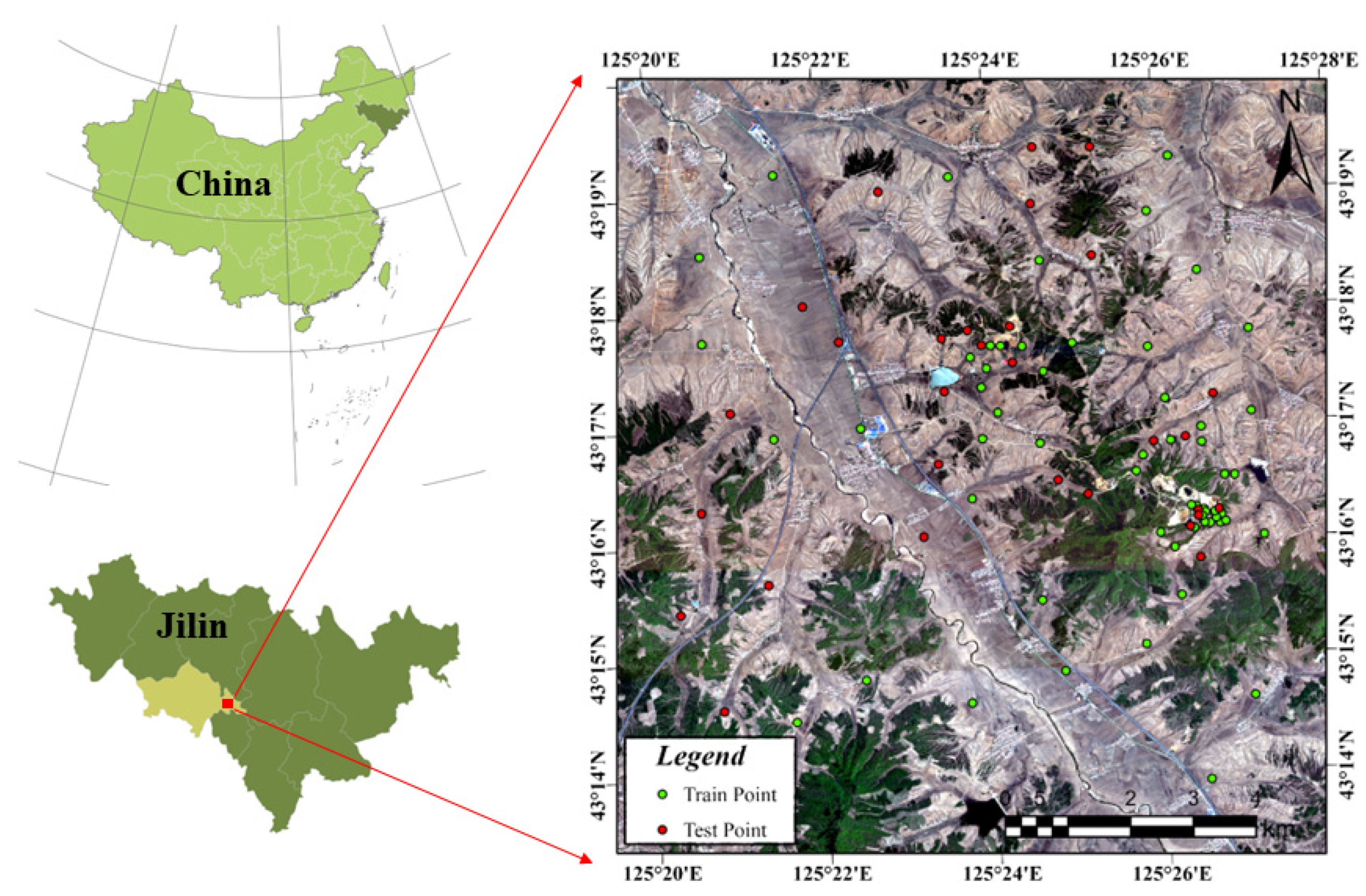
3.1. Datasets and Preprocessing

A total of nine airborne hyperspectral image strip datasets were acquired in the Yitong Manchu Autonomous County in Jilin province, China, between 18 April and 22 April 2017, using a HyMap airborne imaging spectrometer. After stitching, the hyperspectral image data were formed into a spectral cube consisting of 2734 rows, 2508 columns, and 135 bands. The spectral resolution was 10–20 nm, and the spatial resolution was 4.5 m. As is shown in Figure 5, 90 soil samples were sampled simultaneously and were evenly distributed in the study area.

3.1.1. Preprocessing of the Hyperspectral Data Cube

Firstly, to convert the digital number (DN) values into radiometric values that have a physical meaning, the original hyperspectral images were radiometrically calibrated using the standard data obtained by an integrating sphere. After obtaining parameters, such as the atmospheric conditions in the study area, an atmospheric correction was performed using the MODTRAN4 atmospheric radiation transmission model [39]. To solve the problem of geometric distortion, a look-up table was constructed using high-precision position and orientation system (POS) data and digital elevation model (DEM) data. A geometric correction was performed strip by strip, and the photometric correction algorithm based on the bi-directional reflectance distribution function (BRDF) was also used to correct the radiation differences between strips [40]. Finally, a spatial-spectral cube was created with the help of image-stitching technology. As the imagery contained some bands disturbed by water vapor, which are ineffective for the inversion task, the contaminated bands were deleted, and 101 spectral bands were finally retained.

3.1.2. Processing of the Soil Samples

Ninety topsoil samples at depths of 0–20 cm were processed by removing impurities, air-drying, grinding, and 100-mesh sieving. Soil organic carbon content (SOCC) was measured using the K₂Cr₂O₇–H₂SO₄ oxidation method. A conversion factor of 1.724 is commonly used to convert SOCC to SOMC, where SOMC (%) = SOCC (%) × 1.724 [41].

In order to reasonably assess the advantages and disadvantages of the selected features and the inversion accuracy, the 90 samples were divided into training and test sets in a 2:1 ratio, according to the distribution of the SOM.

For spectral preprocessing, the soil spectrum is a combination of various kinds of information, and feature extraction processing can reduce the influence of noise and other interference factors to a certain extent, as well as highlight the feature information. Specifically, continuum removal can be introduced to suppress the background information and normalize the values of weakly absorbed spectra [42], and the first-order differentiation is taken to enhance the correlation between the SOM and the spectrum [6,43]. The band ratio can express the hyperspectral response characteristics of SOM from two-dimensional spectral spaces, which reduces the impact of other soil composition information on the estimation. Therefore, the continuum removal, first-order differentiation, and band ratio were computed for the raw spectrum, and a new set of hyperspectral features was generated by combining the above results, which are explained in the following steps:

(1)

Calculate the absorption depth after continuum removal processing:

$$S_{cr}=S/C$$

(16)

$$D_{cr}=1-S_c$$

(17)

where $S_{cr}$ represents the continuum removal spectrum, $S$ represents the raw spectrum, $C$ represents the continuum curve, and $D_{cr}$ is the absorption depth of the continuum removal.

(2)

Calculate the first-order differentiation of the spectrum:

$$F{D}_i=\frac{S_{i+1}-S_{i-1}}{B_{i+1}-B_{i-1}}$$

(18)

where $S_{i+1}$ and $S_{i-1}$ respectively represent the reflectance of the former and latter bands, $B_{i+1}$ and $B_{i-1}$ respectively represent the wavelength of the former and latter bands, and $F{D}_i$ is the first-order differential value at that band.

(3)

Calculate the band ratio: Since there were 101 bands in the dataset, calculating all the band ratios would result in a large amount of feature redundancy. Therefore, for each band, its ratio to the other bands was calculated, and the ratio with the highest correlation with SOM in all band ratios was selected as the optimal ratio of that band.

(4)

Combine all the above features (raw spectrum, absorption depth of the continuum removal, first-order differentiation, and optimal band ratios).

(5)

Sample expansion based on the spatial distance: Considering Tobler’s first law of geography and the stability of the SOM at the meter level, to improve the model stability, the training set was expanded according to the spatial distance and spectral angle distance from the labeled samples. Unlabeled samples that were spatially neighboring and spectrally close to the training set were added to the new training set.

After processing the soil samples in the spatial and spectral dimensions, 243 training samples and 30 test samples (each with 385 features) were finally obtained.

3.2. Experiment in RLFSR

In this section, we describe how the RLFSR feature selection algorithm was performed on the Yitong airborne hyperspectral dataset. The performance of the two strategies (RLFSR-Net and RLFSR-Cv) with different feature numbers was also tested. Some other popular methods for the dimensionality reduction of hyperspectral data were also performed for comparison. The spectral dimensionality reduction methods involved in the experiments were as follows:

(1)

PCA: principal component analysis, which extracts features to a cumulative contribution rate of 0.99.

(2)

ICA: independent component analysis with 10 components.

(3)

Pearson: the Pearson product-moment correlation coefficient, which selects the 30 characteristics that are most relevant to the dependent variable.

(4)

VIP: variable importance projection, which selects the 30 features of the highest importance for the inversion modeling.

(5)

SOS: symbiotic organisms search.

(6)

IRF: interval random frog.

(7)

CARS: competitive adaptive reweighted sampling.

After acquiring the appropriate features, the accuracy evaluation was performed using four commonly used hyperspectral inversion models:

(1)

PLS: partial least squares regression with 20 latent variables.

(2)

RF: random forest regression, which is a supervised learning algorithm that uses an ensemble learning method for the regression.

(3)

SVM: support vector machine regression equipped with a radial basis function (RBF) kernel. Parameters $\gamma$ and $C$ were determined by 10-fold cross-validation.

(4)

XGBoost: extreme gradient boosting, which is an implementation of gradient-boosted decision trees designed for speed and performance. The main parameters were determined by 10-fold cross-validation.

The coefficient of determination (R²), the MSE, and the MAE were calculated to measure the regression accuracy of the models:

(1)

R²: the coefficient of determination is the proportion of the variation in the dependent variable that is predictable from the independent variable.

(2)

MSE: the mean squared error of an estimator measures the average of the squares of the errors, i.e., the average squared difference between the estimated value and the true value.

(3)

MAE: the mean absolute error is the arithmetic average of the absolute errors.

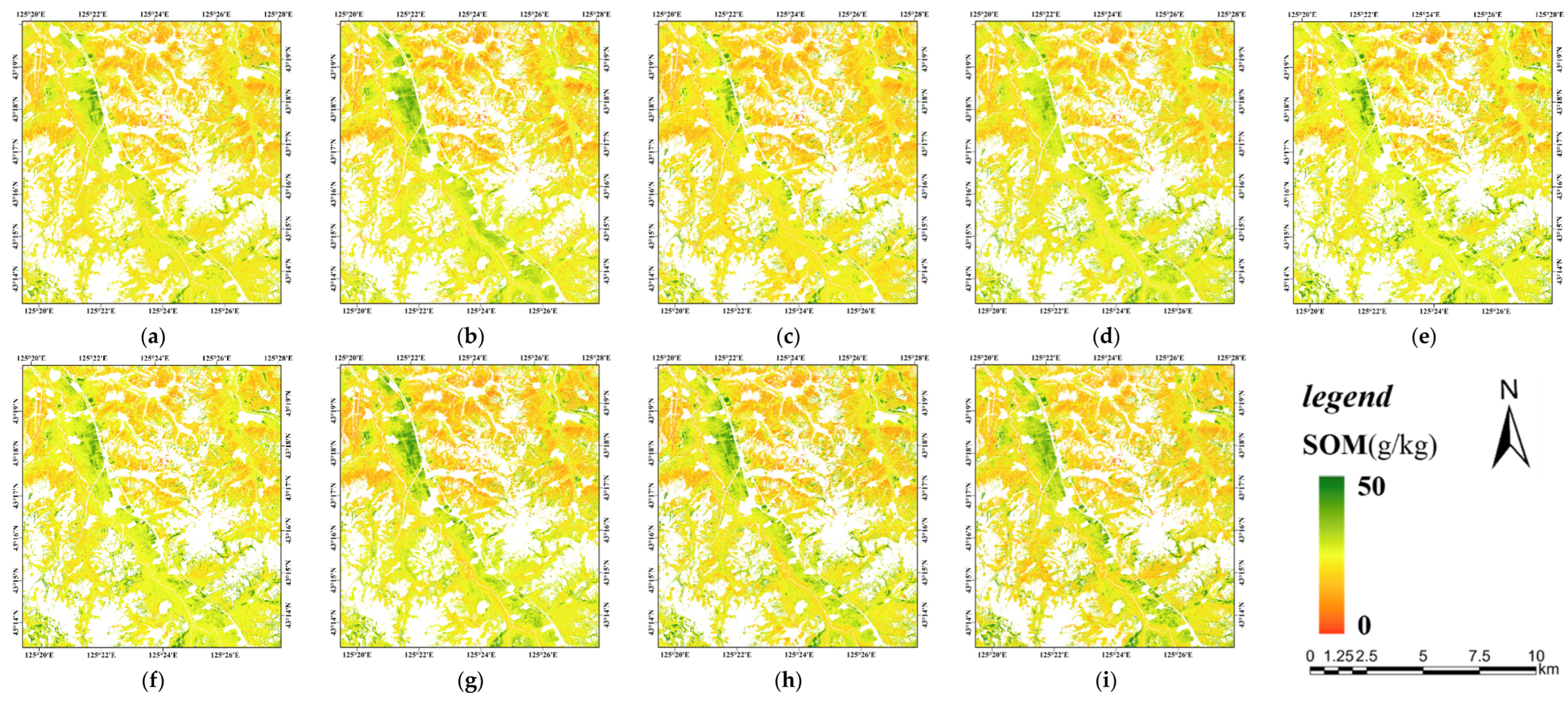
3.3. Results of Different Dimensionality Reduction Methods

The proposed method was evaluated by comparing it with the widely used dimensionality reduction methods described in Section 3.2. For each dimensionality reduction method, the inversion performance was validated for the Yitong airborne hyperspectral dataset, and the accuracy indicators of the selected features obtained using the current model were calculated for the training set and the test set.

From

Table 1. Regression results of PCA, ICA, Pearson, VIP, SOS, IRF, CARS, RLFSR-Net, and RLFSR-Cv using the representative regression models of PLS, SVM-RBF, RF, and XGBoost. The best three regression performances of the dimensionality reduction methods are highlighted in bold, italic, and underlined, respectively.

Method	Regression Model	Training Set			Test Set
		R2	MAE	MSE	R2	MAE	MSE
PCA	PLS	0.5968	3.2967	16.9878	0.3386	3.9512	25.6450
	SVM-RBF	0.9998	0.0989	0.0098	0.0636	4.6384	36.3075
	RF	0.5580	3.3086	18.6191	0.5488	3.3328	17.4946
	XGBoost	0.9729	0.7786	1.1435	0.5332	3.5420	18.0982
ICA	PLS	0.4182	3.9287	24.5114	0.5788	3.2597	16.3295
	SVM-RBF	0.9998	0.0991	0.0099	0.0791	4.6205	35.7049
	RF	0.6942	2.6750	12.8822	0.3452	4.0807	25.3871
	XGBoost	0.8526	1.8588	6.2109	0.3386	3.8821	25.6452
Pearson	PLS	0.4609	3.7721	22.7120	0.4209	3.7285	22.4544
	SVM-RBF	0.6623	2.2414	14.2281	0.5977	3.3790	15.5993
	RF	0.6763	2.8541	13.6371	0.5891	3.1342	15.9333
	XGBoost	0.7929	2.2260	8.7256	0.6122	2.8507	15.0379
VIP	PLS	0.5880	3.3063	17.3584	0.2480	4.0115	29.1573
	SVM-RBF	0.5636	2.9460	18.3826	0.5134	3.3498	18.8654
	RF	0.5861	3.2546	17.4362	0.5579	3.5180	17.1430
	XGBoost	0.9960	0.3060	0.1696	0.5686	3.2672	16.7250
SOS	PLS	0.6217	3.1355	15.9358	0.3224	3.8480	26.2733
	SVM-RBF	0.8166	1.5208	7.7243	0.4664	3.7999	20.6903
	RF	0.7841	2.3960	9.0969	0.5541	3.5191	17.2875
	XGBoost	0.9999	0.0472	0.0043	0.5024	3.6873	19.2929
IRF	PLS	0.7738	2.4291	9.5302	0.0012	5.4822	57.2887
	SVM-RBF	0.9211	0.7375	3.3228	0.5682	3.1987	16.7439
	RF	0.7910	2.3532	8.8043	0.6649	3.0512	12.9923
	XGBoost	0.9999	0.0470	0.0041	0.6514	2.9768	13.5181
CARS	PLS	0.7418	2.6394	10.8791	0.0018	4.9548	44.3211
	SVM-RBF	0.8302	1.4981	7.1515	0.6902	2.8810	12.0125
	RF	0.6943	2.8585	12.8799	0.6541	2.9864	13.4113
	XGBoost	0.9750	0.7535	1.0512	0.6228	2.9414	14.6253
RLFSR-Net	PLS	0.5211	3.4638	20.1745	0.4080	3.6995	22.9549
	SVM-RBF	0.7514	1.8932	10.4742	0.6955	2.7447	11.8063
	RF	0.7320	2.5578	11.2919	0.7312	2.6398	10.4218
	XGBoost	0.9999	0.0006	0.0001	0.7506	2.7276	9.6700
RLFSR-Cv	PLS	0.5390	3.4213	19.4200	0.3960	3.3683	23.4192
	SVM-RBF	0.7227	2.0551	11.6808	0.6549	2.9157	13.3790
	RF	0.7739	2.3723	9.5260	0.6800	2.8373	12.4054
	XGBoost	0.9997	0.0735	0.0108	0.7518	2.4512	9.6215

, it can be seen that ICA had the worst performance among the seven methods, mainly because the uncertainty of the energy and the order of the independent components led to a failure to effectively eliminate irrelevant information. In contrast, PCA removed the noise while retaining most of the information, thus achieving effective dimensionality reduction, but its extracted features could not explain the spectral characteristics of the SOM. These signal-processing techniques are oriented to retain as much information as possible and are not optimized for specific tasks, so the extracted features cannot always effectively represent the spectral response of SOM. The Pearson and VIP methods evaluate the importance of each feature with different metrics, and select the most important features to form the subset of features. As a result, these two methods achieved high-precision inversion with the XGBoost model. The SOS algorithm simulates the symbiotic interaction strategies that organisms use to survive in the ecosystem [44], but it performed poorly. The IRF provided satisfactory prediction results, but over 100 features were selected, and the dimensionality reduction task was not well accomplished. The proposed methods of RLFSR-Net and RLFSR-Cv obtained the best prediction accuracy, with at least a 0.05 increase in R² on the test set. Based on the XGBoost model, the two methods yielded similar prediction results, with R² exceeding 0.75, which represents very high accuracy. The PLS model achieved worse inversion results than SVM, RF, and XGBoost, which is shown in Table 1. PLS regression employs independent variables to extract latent variables and conducts regression modeling; thus, the redundant features selected by IRF and CARS will have a greater impact on the generation of latent variables. The DRL-based algorithms incorporate the SOM prediction accuracy into the optimization metric and can effectively explore the optimal subset of features for the current scenario, which is the most applicable to SOM inversion modeling. Since RLFSR-Cv utilizes the cross-validation accuracy of the XGBoost model to evaluate the feature subset when selecting features, its performance on the XGBoost model was naturally better than that of the RLFSR-Net, but it was relatively slightly worse for other regression models. Furthermore, in RLFSR-Net, the specially designed accuracy evaluation network greatly improves the stability of the feature subset under different inversion models. As a result, the extracted spectral features showed better accuracy under multiple models, and the evaluation policy of multiple cross-validations in RLFSR-Cv also had a similar effect. In conclusion, the two proposed feature selection methods realized stable and excellent dimensionality reduction by introducing 10-fold cross-validation and an evaluation network trained by random features, respectively.

In Figure 6, the SOM prediction maps obtained from the best models of different feature reduction methods are plotted. Many methods demonstrated an overall high (ICA) or low (PCA, Pearson, VIP, SOS, and IRF) bias in SOM predictions. In contrast, the CARS and DRL-based methods demonstrated excellent cartographic results, and they accurately characterized the spatial distribution of the SOM in the study area. The CARS and proposed methods indicated a zone of high SOM values in the study area extending from the northwest to the southeast. When compared with CARS, the proposed methods captured the spatial differences of the SOM more clearly, and the distribution of the high-value regions was also more apparent, which demonstrated the superior performance of the proposed methods in the spectral feature recognition task.

Table 2. Comparation of the computational times on different methods.

Method	Inference Time (s)
PCA	0.04
ICA	0.10
Pearson	0.01
VIP	0.12
CARS	22.96
SOS	353.46
IRF	397.84
RLFSR-Cv	177.51
RLFSR-Net	92.97

shows the inference time of the proposed DRL-based method and other dimensionality reduction methods. Some dimensionality reduction methods do not include a feature subset collection process; hence, they have short inference times and the effectiveness is also relatively limited, e.g., PCA, ICA, Pearson and VIP. Other methods include feature subset generation and feature subset evaluation and have longer inference times. The proposed method consumes a relatively small amount of inference time.

4. Discussion

4.1. Performance with Different Numbers of Selected Features

For the dimensionality reduction methods with a constant number of features, we explored their prediction performance with different feature subsets. Since the SVM-RBF and XGBoost regression models demonstrated satisfactory accuracy in the experiments described in Section 4.1, we explored the performance of several dimensionality reduction methods with the SVM-RBF and XGBoost regression models. As is shown in Figure 7, in general, the inversion accuracy improved as the number of features increased, but the accuracy of each model stabilized or decreased slightly beyond 40 features, which was probably due to the gradual redundancy of features. Modeling with all features did not yield a satisfactory prediction, with the R² below 0.6. The prediction accuracy of the VIP method was poor, and no suitable spectral features were effectively extracted. The spectral extraction method based on the Pearson’s correlation coefficient showed a more stable inversion accuracy with a different number of features, but due to the strong correlation within the spectral features, increasing the number of selected features may not have resulted in consistent changes in the spectral information, i.e., the added spectral features were mostly redundant information. The CARS method was quite random in generating feature subsets and achieved good prediction accuracy after several iterations. The proposed RLFSR-Net and RLFSR-Cv methods achieved better feature selection results than the VIP and Pearson methods, and they achieved a close or better R² for each number of features.

Both the SVM-RBF and XGBoost regression models provided excellent prediction accuracy, but the two proposed methods obtained better performance with XGBoost, and achieved higher R² values and better prediction results than the CARS method. Therefore, we analyzed the regression results of RLFSR on different numbers of features in

Table 3. Regression Results of RLFSR on different number of features.

Method	Number of Features	Training Set			Test Set
		R2	MAE	MSE	R2	MAE	MSE
RLFSR-Net	10	0.9977	0.2144	0.0959	0.4514	3.7140	21.2701
	15	0.9991	0.1346	0.0364	0.6758	2.6654	12.5721
	20	0.9989	0.1518	0.0457	0.6609	3.0678	13.1479
	25	0.9995	0.1097	0.0223	0.7055	2.9341	11.4206
	30	0.9995	0.1003	0.0205	0.7103	2.8101	11.2323
	35	0.9999	0.0006	0.0001	0.7506	2.7276	9.6700
	40	0.9997	0.0742	0.0111	0.7171	2.3913	10.9676
	45	0.9998	0.0685	0.0097	0.7044	2.9024	11.4620
	50	0.9999	0.0556	0.0058	0.6690	3.0277	12.8336
RLFSR-Cv	10	0.9985	0.1862	0.0624	0.4876	3.6880	19.8690
	15	0.9996	0.0848	0.0154	0.5100	3.7000	18.9994
	20	0.9994	0.1113	0.0254	0.6744	2.6709	12.6227
	25	0.9997	0.0764	0.0122	0.6886	2.9802	12.0740
	30	0.9997	0.0825	0.0125	0.6529	2.9904	13.4596
	35	0.9997	0.0735	0.0108	0.7518	2.4512	9.6215
	40	0.9999	0.0480	0.0052	0.7362	2.3955	10.2286
	45	0.9999	0.0563	0.0060	0.6949	2.8559	11.8290
	50	0.9999	0.0473	0.0042	0.6710	2.9491	12.7550

. When the number of features reached 35, RLFSR-Net and RLFSR-Cv achieved the highest inversion accuracy at 35 features, with R² values of 0.7506 and 0.7518, respectively. Both methods failed to select suitable features and showed poor inversion accuracy with XGBoost when too few features were selected. When the number of features exceeded 35, the spectral feature information started to appear redundant, which led to a slight decrease in prediction accuracy.

4.2. Analysis of the Spectral Features

To further explore the value of the proposed framework in SOM prediction, we extracted the distribution of the selected feature subsets. Figure 8 plots the spectral features of the 90 soil samples and annotates the locations of the feature subsets selected by the three best-performing algorithms. The CARS method selected more than 70 features, which was far more than the 35 features of the RLFSR-Net and RLFSR-Cv, and it mainly focused on the 2.2 μm area of the original spectrum and the other preprocessed spectra. In the original spectrum, the proposed RLFSR methods tended to extract features at 0.5 μm, 0.8 μm, and 2.2 μm, which was consistent with the distribution range of spectral characteristics of the SOM found by some scholars [6,45,46,47,48]. For the pre-processed spectra, the SOM spectral features appeared in the same position as the original spectrum. However, from Figure 8b,c, it can be clearly observed that there are more significant peaks in the visible range and in the 2.2 µm range, which demonstrated the vital enhancement of the pre-processing method for extracting spectral features.

Generally, the feature subsets of the three methods had relatively high consistency, and the feature subset of the CARS method contained most of the spectral features of RLFSR-Net and RLFSR-Cv. However, when compared with the CARS method, the two proposed methods exhibited better prediction accuracy on multiple models and significantly reduced the size of the feature subset. The large reward for the feature subset prediction accuracy in Markov modeling makes the RLFSR-Net and RLFSR-Cv algorithms more inclined to search for the spectral features that contribute the most to the SOM prediction, while limiting the number of features that do not contribute much to SOM prediction. This design enables the proposed methods to fully characterize the SOM distribution with a small feature subset, which improves the accuracy of SOM inversion while suppressing information redundancy with excellent performance.

A comparison of the two proposed methods shows that RLFSR-Net selected several spectral features in nearby bands, while RLFSR-Cv avoided the duplicate selection of similar features as much as possible. This discrepancy can be attributed to the difference in the preference for the agents’ reward policies in the design of reinforcement learning. In RLFSR-Net, an environment is designed where the prediction accuracy of the pre-trained network serves as a reward. Meanwhile, in RLFSR-Cv, an environment that includes a greater variety of rewards and punishments is proposed, for which the correlation coefficient serves as the negative reward and the cross-validation accuracy serves as the active reward. By fine-tuning the interaction behavior of the reinforcement learning agents with the environment, the model’s preference in feature selection changes correspondingly, and the selected feature subsets demonstrated an excellent SOM inversion performance.

5. Conclusions

In this paper, we have proposed a feature selection method using reinforcement learning as a framework (RLFSR) to address the problem of unclear features in airborne hyperspectral SOM regression. To model the feature subset selection process, an MDP was formulated. Two feature evaluation structures were proposed by introducing a pre-trained evaluation network and a cross-validation technique, respectively. In RLFSR-Net, the spectral features were randomly fed to train a deep regression network, and the performance of the reinforcement learning agent was measured using the prediction error for a subset of features in the deep network. In contrast, 10-fold cross-validation was used in RLFSR-Cv to evaluate the feature subset and add a suppression condition for the inter-feature correlation. Through this design, unique and valuable spectral features could be effectively selected. The effectiveness of the proposed methods was demonstrated using HyMap airborne hyperspectral data from the Yitong Manchu Autonomous County in China. The extracted feature subsets performed well in each inversion model, while outperforming commonly used feature selection methods, such as CARS, which demonstrated the better stability of the proposed framework and obtained the best inversion results with the XGBoost model. The R² values for RLFSR-Net and RLFSR-Cv were 0.7506 and 0.7518, respectively. The DRL-based method and CARS method both demonstrated good accuracy in the SOM mapping, but the two proposed methods extracted more concise and efficient subsets of features, which makes them better for the feature selection task. By flexibly setting the reward strategy of reinforcement learning, the proposed methods showed different performances, with RLFSR-Cv demonstrating better results in suppressing the repetitive selection of similar features. In our future work, optimizing the feature evaluation policies for different applications will be an exciting application of reinforcement learning in hyperspectral inversion.

References

1. Bünemann, E.K.; Bongiorno, G.; Bai, Z.; Creamer, R.E.; De Deyn, G.; de Goede, R.; Fleskens, L.; Geissen, V.; Kuyper, T.W.; Mäder, P. Soil quality–A critical review. Soil Biol. Biochem. 2018, 120, 105–125. [Google Scholar] [CrossRef]
2. Tan, K.; Ma, W.; Chen, L.; Wang, H.; Du, Q.; Du, P.; Yan, B.; Liu, R.; Li, H. Estimating the distribution trend of soil heavy metals in mining area from HyMap airborne hyperspectral imagery based on ensemble learning. J. Hazard. Mater. 2021, 401, 123288. [Google Scholar] [CrossRef] [PubMed]
3. Tan, K.; Wang, H.; Chen, L.; Du, Q.; Du, P.; Pan, C. Estimation of the spatial distribution of heavy metal in agricultural soils using airborne hyperspectral imaging and random forest. J. Hazard. Mater. 2020, 382, 120987. [Google Scholar] [CrossRef] [PubMed]
4. Meng, X.; Bao, Y.; Ye, Q.; Liu, H.; Zhang, X.; Tang, H.; Zhang, X. Soil organic matter prediction model with satellite hyperspectral image based on optimized denoising method. Remote Sens. 2021, 13, 2273. [Google Scholar] [CrossRef]
5. Nanni, M.R.; Demattê, J.A.M.; Rodrigues, M.; Santos, G.L.A.A.d.; Reis, A.S.; Oliveira, K.M.d.; Cezar, E.; Furlanetto, R.H.; Crusiol, L.G.T.; Sun, L. Mapping particle size and soil organic matter in tropical soil based on hyperspectral imaging and non-imaging sensors. Remote Sens. 2021, 13, 1782. [Google Scholar] [CrossRef]
6. Ou, D.; Tan, K.; Lai, J.; Jia, X.; Wang, X.; Chen, Y.; Li, J. Semi-supervised DNN regression on airborne hyperspectral imagery for improved spatial soil properties prediction. Geoderma 2021, 385, 114875. [Google Scholar] [CrossRef]
7. Kumar, V.; Minz, S. Feature selection: A literature review. SmartCR 2014, 4, 211–229. [Google Scholar] [CrossRef]
8. Lee, J.; Park, D.; Lee, C. Feature selection algorithm for intrusions detection system using sequential forward search and random forest classifier. KSII Trans. Internet Inf. Syst. (TIIS) 2017, 11, 5132–5148. [Google Scholar]
9. Marcano-Cedeño, A.; Quintanilla-Domínguez, J.; Cortina-Januchs, M.; Andina, D. Feature selection using sequential forward selection and classification applying artificial metaplasticity neural network. In Proceedings of the IECON 2010-36th Annual Conference on IEEE Industrial Electronics Society, Glendale, AZ, USA, 7–10 November 2010; pp. 2845–2850. [Google Scholar]
10. Ververidis, D.; Kotropoulos, C. Sequential forward feature selection with low computational cost. In Proceedings of the 2005 13th European Signal Processing Conference, Antalya, Turkey, 4–8 September 2005; pp. 1–4. [Google Scholar]
11. Mao, K.Z. Orthogonal forward selection and backward elimination algorithms for feature subset selection. IEEE Trans. Syst. Man Cybern. Part B Cybern. 2004, 34, 629–634. [Google Scholar] [CrossRef]
12. Cotter, S.F.; Kreutz-Delgado, K.; Rao, B.D. Backward sequential elimination for sparse vector subset selection. Signal Process. 2001, 81, 1849–1864. [Google Scholar] [CrossRef]
13. Dash, M.; Liu, H. Feature selection for classification. Intell. Data Anal. 1997, 1, 131–156. [Google Scholar] [CrossRef]
14. Shafiee, S.; Lied, L.M.; Burud, I.; Dieseth, J.A.; Alsheikh, M.; Lillemo, M. Sequential forward selection and support vector regression in comparison to LASSO regression for spring wheat yield prediction based on UAV imagery. Comput. Electron. Agric. 2021, 183, 106036. [Google Scholar] [CrossRef]
15. Meiri, R.; Zahavi, J. Using simulated annealing to optimize the feature selection problem in marketing applications. Eur. J. Oper. Res. 2006, 171, 842–858. [Google Scholar] [CrossRef]
16. Huang, C.-L.; Wang, C.-J. A GA-based feature selection and parameters optimizationfor support vector machines. Expert Syst. Appl. 2006, 31, 231–240. [Google Scholar] [CrossRef]
17. De La Iglesia, B. Evolutionary computation for feature selection in classification problems. Wiley Interdiscip. Rev. Data Min. Knowl. Discov. 2013, 3, 381–407. [Google Scholar] [CrossRef]
18. Xue, B.; Zhang, M.; Browne, W.N. Particle swarm optimization for feature selection in classification: A multi-objective approach. IEEE Trans. Cybern. 2012, 43, 1656–1671. [Google Scholar] [CrossRef]
19. Wang, X.; Yang, J.; Teng, X.; Xia, W.; Jensen, R. Feature selection based on rough sets and particle swarm optimization. Pattern Recognit. Lett. 2007, 28, 459–471. [Google Scholar] [CrossRef] [Green Version]
20. Zabinsky, Z.B. Random Search Algorithms; Department of Industrial and Systems Engineering, University of Washington: Washinton, DC, USA, 2009. [Google Scholar]
21. Almuallim, H.; Dietterich, T.G. Learning boolean concepts in the presence of many irrelevant features. Artif. Intell. 1994, 69, 279–305. [Google Scholar] [CrossRef]
22. Ben-Bassat, M. Pattern recognition and reduction of dimensionality. Handb. Stat. 1982, 2, 773–910. [Google Scholar]
23. Devijver, P.A.; Kittler, J. Pattern Recognition: A Statistical Approach; Prentice Hall: Hoboken, NJ, USA, 1982. [Google Scholar]
24. Hall, M.A. Correlation-Based Feature Selection of Discrete and Numeric Class Machine Learning; University of Waikato: Hamilton, New Zealand, 2000. [Google Scholar]
25. Hall, M.A. Correlation-Based Feature Selection for Machine Learning. Ph.D. Thesis, The University of Waikato, Hamilton, New Zealand, 1999. [Google Scholar]
26. Piramuthu, S. Evaluating feature selection methods for learning in data mining applications. Eur. J. Oper. Res. 2004, 156, 483–494. [Google Scholar] [CrossRef]
27. Liu, H.; Motoda, H. Feature Selection for Knowledge Discovery and Data Mining; Springer Science & Business Media: Berlin/Heidelberg, Germany, 2012; Volume 454. [Google Scholar]
28. John, G.H.; Kohavi, R.; Pfleger, K. Irrelevant features and the subset selection problem. In Machine Learning Proceedings 1994; Elsevier: Amsterdam, The Netherlands, 1994; pp. 121–129. [Google Scholar]
29. Bangelesa, F.; Adam, E.; Knight, J.; Dhau, I.; Ramudzuli, M.; Mokotjomela, T.M. Predicting soil organic carbon content using hyperspectral remote sensing in a degraded mountain landscape in lesotho. Appl. Environ. Soil Sci. 2020, 2020, 2158573. [Google Scholar] [CrossRef]
30. Song, Y.-Q.; Zhao, X.; Su, H.-Y.; Li, B.; Hu, Y.-M.; Cui, X.-S. Predicting spatial variations in soil nutrients with hyperspectral remote sensing at regional scale. Sensors 2018, 18, 3086. [Google Scholar] [CrossRef] [PubMed]
31. Wei, L.; Yuan, Z.; Zhong, Y.; Yang, L.; Hu, X.; Zhang, Y. An improved gradient boosting regression tree estimation model for soil heavy metal (Arsenic) pollution monitoring using hyperspectral remote sensing. Appl. Sci. 2019, 9, 1943. [Google Scholar] [CrossRef] [Green Version]
32. Kawamura, K.; Tsujimoto, Y.; Nishigaki, T.; Andriamananjara, A.; Rabenarivo, M.; Asai, H.; Rakotoson, T.; Razafimbelo, T. Laboratory visible and near-infrared spectroscopy with genetic algorithm-based partial least squares regression for assessing the soil phosphorus content of upland and lowland rice fields in Madagascar. Remote Sens. 2019, 11, 506. [Google Scholar] [CrossRef] [Green Version]
33. Feng, J.; Li, D.; Chen, J.; Zhang, X.; Tang, X.; Wu, X. Hyperspectral band selection based on ternary weight convolutional neural network. In Proceedings of the IGARSS 2019—2019 IEEE International Geoscience and Remote Sensing Symposium, Yokohama, Japan, 28 July–2 August 2019; pp. 3804–3807. [Google Scholar]
34. Lorenzo, P.R.; Tulczyjew, L.; Marcinkiewicz, M.; Nalepa, J. Hyperspectral band selection using attention-based convolutional neural networks. IEEE Access 2020, 8, 42384–42403. [Google Scholar] [CrossRef]
35. Ortiz, A.; Granados, A.; Fuentes, O.; Kiekintveld, C.; Rosario, D.; Bell, Z. Integrated learning and feature selection for deep neural networks in multispectral images. In Proceedings of the IEEE Conference on Computer Vision and Pattern Recognition Workshops, Salt Lake City, UT, USA, 18–22 June 2018; pp. 1196–1205. [Google Scholar]
36. Bernal, E.A. Surrogate Contrastive Network for Supervised Band Selection in Multispectral Computer Vision Tasks. In Proceedings of the IEEE/CVF Conference on Computer Vision and Pattern Recognition Workshops, Long Beach, CA, USA, 16–17 June 2019. [Google Scholar]
37. Mou, L.; Saha, S.; Hua, Y.; Bovolo, F.; Bruzzone, L.; Zhu, X.X. Deep reinforcement learning for band selection in hyperspectral image classification. IEEE Trans. Geosci. Remote Sens. 2021, 60, 5504414. [Google Scholar] [CrossRef]
38. Feng, J.; Li, D.; Gu, J.; Cao, X.; Shang, R.; Zhang, X.; Jiao, L. Deep reinforcement learning for semisupervised hyperspectral band selection. IEEE Trans. Geosci. Remote Sens. 2021, 60, 5501719. [Google Scholar] [CrossRef]
39. Berk, A.; Anderson, G.P.; Bernstein, L.S.; Acharya, P.K.; Dothe, H.; Matthew, M.W.; Adler-Golden, S.M.; Chetwynd, J.H., Jr.; Richtsmeier, S.C.; Pukall, B. MODTRAN4 radiative transfer modeling for atmospheric correction. In Proceedings of the Optical Spectroscopic Techniques and Instrumentation for Atmospheric and Space Research III, Denver, CO, USA, 19–21 July 1999; pp. 348–353. [Google Scholar]
40. Yu, J.; Yan, B.; Liu, W.; Li, Y.; He, P. Seamless Mosaicking of Multi-strip Airborne Hyperspectral Images Based on Hapke Model. In Proceedings of the International Conference on Sensing and Imaging, Chengdu, China, 5–7 June 2017; pp. 285–292. [Google Scholar]
41. Wang, X.; Zhang, F.; Johnson, V.C. New methods for improving the remote sensing estimation of soil organic matter content (SOMC) in the Ebinur Lake Wetland National Nature Reserve (ELWNNR) in northwest China. Remote Sens. Environ. 2018, 218, 104–118. [Google Scholar] [CrossRef]
42. Mutanga, O.; Skidmore, A.K.; Prins, H. Predicting in situ pasture quality in the Kruger National Park, South Africa, using continuum-removed absorption features. Remote Sens. Environ. 2004, 89, 393–408. [Google Scholar] [CrossRef]
43. Dou, X.; Wang, X.; Liu, H.; Zhang, X.; Meng, L.; Pan, Y.; Yu, Z.; Cui, Y. Prediction of soil organic matter using multi-temporal satellite images in the Songnen Plain, China. Geoderma 2019, 356, 113896. [Google Scholar] [CrossRef]
44. Jaffel, Z.; Farah, M. A symbiotic organisms search algorithm for feature selection in satellite image classification. In Proceedings of the 2018 4th International Conference on Advanced Technologies for Signal and Image Processing (ATSIP), Sousse, Tunisia, 21–24 March 2018; pp. 1–5. [Google Scholar]
45. Liu, H.; Zhang, Y.; Zhang, B. Novel hyperspectral reflectance models for estimating black-soil organic matter in Northeast China. Environ. Monit. Assess. 2009, 154, 147–154. [Google Scholar] [CrossRef] [PubMed]
46. Weidong, L.; Baret, F.; Xingfa, G.; Qingxi, T.; Lanfen, Z.; Bing, Z. Relating soil surface moisture to reflectance. Remote Sens. Environ. 2002, 81, 238–246. [Google Scholar] [CrossRef]
47. Shen, L.; Gao, M.; Yan, J.; Li, Z.-L.; Leng, P.; Yang, Q.; Duan, S.-B. Hyperspectral estimation of soil organic matter content using different spectral preprocessing techniques and PLSR method. Remote Sens. 2020, 12, 1206. [Google Scholar] [CrossRef] [Green Version]
48. Ou, D.; Tan, K.; Wang, X.; Wu, Z.; Li, J.; Ding, J. Modified soil scattering coefficients for organic matter inversion based on Kubelka-Munk theory. Geoderma 2022, 418, 115845. [Google Scholar] [CrossRef]
Figure 1. The proposed RLFSR framework.
Remotesensing 15 00127 g001
Figure 2. Feature evaluation framework of RLFSR-Net.
Remotesensing 15 00127 g002
Figure 3. Feature evaluation framework of the RLFSR-Cv.
Remotesensing 15 00127 g003
Figure 4. The architecture of the A2C-based network.
Remotesensing 15 00127 g004
Figure 5. Study area.
Remotesensing 15 00127 g005
Figure 6. SOM prediction maps for Yitong Manchu Autonomous County. (a) PCA. (b) ICA. (c) Pearson. (d) VIP. (e) SOS. (f) IRF. (g) CARS. (h) RLFSR-Net. (i) RLFSR-Cv.
Remotesensing 15 00127 g006
Figure 7. R2 curves of the different feature selection methods. The x-axis indicates the number of features, and the y-axis indicates the R2 obtained from the test set. (a) R2 of the SVM-RBF model. (b) R2 of the XGBoost model.
Remotesensing 15 00127 g007
Figure 8. The features selected by the different methods: CARS (blue), RLFSR-Net (orange), and RLFSR-Cv (gray). The x-axis indicates the wavelength. The spectral features are (a) the original spectrum, (b) the absorption depth of continuum removal, (c) the first derivative, and (d) the band ratio.
Remotesensing 15 00127 g008aRemotesensing 15 00127 g008b