Article

A Mesh Mapping-Based Cooperative Inversion Strategy for Airborne Transient Electromagnetic and Magnetic Methods

1
CAS Engineering Laboratory for Deep Resources Equipment and Technology, Institute of Geology and Geophysics, Chinese Academy of Sciences, Beijing 100029, China
2
Innovation Academy for Earth Science, CAS, Beijing 100029, China
3
College of Earth and Planetary Sciences, University of Chinese Academy of Sciences, Beijing 100049, China
*
Author to whom correspondence should be addressed.
Remote Sens. 2023, 15(1), 125; https://doi.org/10.3390/rs15010125
Submission received: 6 November 2022 / Revised: 14 December 2022 / Accepted: 22 December 2022 / Published: 26 December 2022

Abstract

:
Cooperative inversion is a powerful underground imaging technique that can overcome the limitations of a single detection method. However, due to the different grid divisions used by various geophysical methodologies, imposing structural constraints between grids of different scales is challenging. This paper proposes a new cooperative inversion strategy and applies it to the inversion of the quasi-two-dimensional aerial transient electromagnetic method (ATEM) with the induced polarization (IP) effect and the two-dimensional magnetic method to solve the problem of applying cross-gradient constraints under grids of different scales. The mesh mapping method is incorporated into the iterative process of cooperative inversion in this inversion strategy. The inversion of synthetic data shows that this technique can effectively employ data complementarity to increase the accuracy of the results for describing the medium boundary. The mesh mapping methodology may be applied to the cooperative inversion of geophysical methods under any grid division and successfully solves the problem of grid division mismatch in cooperative inversion.

1. Introduction

Geophysical inversion is an effective method for determining the structure of underground media. However, since conventional geophysical exploration methods can only be applied on the surface and the inverse problem is poorly posed, it is often difficult to solve the geophysical inverse problem accurately [1]. Furthermore, different geophysical methods are sensitive to different underground features. Since the 1970s, several researchers have blended various geophysical approaches to reflect the structural properties of subsurface media [2,3,4]. Multidata inversion can be divided into joint inversion [5,6,7] and cooperative inversion [8,9,10], with the goal of increasing constraints and prior information in the inversion to improve the inversion results [11]. Physical constraints and structural limitations are two types of restrictions. Imposing physical property restrictions involves using an empirical relationship or statistical law between a rock’s physical quality and the inversion results during the inversion process in order to constrain the inversion results and improve the accuracy of the inversion results. The empirical relationship includes the Archie formula [12] and Faust relation [13]. Gao [14] utilized Archie’s formula to link resistivity, velocity, porosity, and other petrophysical characteristics in order to invert electromagnetic and seismic data simultaneously. Such petrophysical relationships, however, are usually discovered through the statistical analysis of borehole and core data, and the physical relationships obtained in different regions are typically divergent. Jegen [15] investigated resistivity and p-wave velocity and discovered a piecewise empirical relationship between physical property parameters. As can be seen, due to the complexity of the Earth’s medium, this empirical relationship has some limitations, and an empirical formula can only be used within the range of its corresponding physical properties. Simultaneously, many researchers have proposed and applied the structural constraint method to the joint inversion of various geophysical methods, such as the model curvature constraint [16], cross-gradient constraint [17], and model gradient dot product [18]. Gallardo and Meju’s proposed cross-gradient constraint can judge the similarity of structures based on the gradient information, obtaining more structurally similar inversion results. Using the cross-gradient constraint, many researchers have achieved good results in the joint inversion of different geophysical methods [19,20,21]. However, this type of joint inversion approach typically requires the use of the same grid subdivision, which makes it difficult to directly apply it to other geophysical methods with grid mismatch. Furthermore, due to the large number of geophysical forward and inverse calculations in a high-dimensional case compared to a one-dimensional case [22,23,24,25], the joint inversion is usually a multiparameter inversion, which further increases the cost compared to a single parameter inversion; therefore, a three-dimensional joint inversion is difficult to be widely used in the fine inversion of underground media at the moment.
Negative values will appear in the data of late traces when using the ATEM to detect some metal mining areas [26]. This phenomenon is caused by the IP characteristics of rocks and ores [27]. The negative response cannot be explained by conventional resistivity inversion methods. The complex resistivity inversion method based on the Cole–Cole model [28] not only improves the inversion accuracy but also provides IP parameter information [29]. One-dimensional inversion methods based on layered media, on the other hand, are usually discontinuous in the transverse direction. The concept of lateral constraint [30] is widely used in a quasi-two-dimensional inversion of various electromagnetic technologies to improve the dependability results. The ATEM laterally constrained inversion, taking into consideration the IP characteristics of rocks and ores, provides more geological information, but the complexity of the inversion also increases, resulting in a greater inversion difficulty. Accurate IP parameters cannot be obtained from aircraft IP response data [31]. Magnetic exploration can be carried out simultaneously with aircraft TEM exploration activity. However, the magnetic exploration inversion interpretation suffers from a lack of vertical resolution [32]. Some researchers have used the weight function to improve its resolution in the depth direction, but the parameters of the depth weight function still depend heavily on the accuracy of prior information [33].
In this research, we present a new cooperative inversion strategy that incorporates the mesh mapping method into the sequential inversion. This method effectively solves the problem of unmatched grid division in the cooperative inversion of different geophysical methods, and it can also combine one-dimensional inversion with high-dimensional inversion for faster cooperative inversion. We used this method to improve on the original inversion results of the quasi-2D ATEM method and the 2D magnetic method. To begin, the IP characteristics of rock and ore were taken into consideration in the one-dimensional forward inversion of the ATEM, and the quasi-two-dimensional damped least squares inversion was completed using the concept of lateral constraint. The analytical formula was then utilized to perform two-dimensional forward modeling using the magnetic method. The magnetic method of inversion is similar to the TEM inversion. Finally, the concepts of mesh mapping and cross-gradient were introduced in order to perform the cooperative inversion of the two approaches. To evaluate the effectiveness of the cooperative inversion, the single inversion and the cooperative inversion were calculated for the synthetic data. It was discovered that the cooperative inversion algorithm can effectively improve the inversion quality.

2. Methods

2.1. Inversion of the Quasi-2D ATEM with IP Effect

The ATEM forward modeling is based on the numerical integral formula of one-dimensional layered media [34].
H z = I a 2 0 e λ z + h + r T E e λ z h λ J 1 λ a d λ
In terms of inversion, this research study adopted the logarithmic parameter transformation function [35] for the parameter range constraint, followed by damped least squares inversion [36]. The objective function of inversion is
Φ = W d d o b s F m + λ W m m
where d o b s represents the observed data, F m represents the forward operator, m represents the model parameter, λ is the regularization factor, and   W d and W m represent the data weighting term and model weighting term, respectively. Using the derivative of the objective function to calculate the minimum, the inversion formula is:
Δ m = J T C d J + λ C m 1 J T C m f m 0 d o b s
where J is Jacobian matrix, which could be computed analytically; C d and C m are the data weighting matrix and model weighting matrix, respectively.
C d = d i a g 1 δ
C z m = W T W
where W is the difference matrix, and δ represents the standard deviation of the data.
Each inversion iteration requires a substantial amount of time to calculate the Jacobian matrix. This work obtained the frequency domain analytical formulation of the Jacobian matrix of the inversion parameters, followed by the time domain Jacobian matrix required for the inversion using sine transformation.
One-dimensional inversion was used to derive the model thickness, resistivity, chargeability, time constant, and frequency dependence. A three-layer model was designed for testing in this research. The thicknesses of the first layer and the second layer were 60 and 90 m, respectively. The resistivity of the three layers was 100, 50, and 200   Ω · m ; the chargeability was 0.1, 0.5, and 0.1; the time constant was 0.00, 0.004, and 0.002   s ; and the frequency dependence was 0.1, 0.3, and 0.1, respectively. To determine the model parameters in the inversion, we designed ten layers of media in the inversion.
The inversion results shown in Figure 1 illustrate that the resistivity inversion effect was the best, and it was more consistent with the true geoelectric structure. The second result was the chargeability inversion, which might reflect the existence of underground IP bodies as well as a trend of abnormal alterations. Due to the fact of their low sensitivity and weak inversion effect, the frequency correlation coefficient and the time constant can be used as auxiliary data to participate in interpretation in combination with the charge-ability results. The conclusions of the inversion are consistent with Viezzoli’s [37] numerical simulation conclusion.
The underground stratum interface was generally distributed horizontally and continuously in the shallow sedimentary environment. The ATEM’s measurement points were close together, and the physical property difference between them was often insignificant. The basic idea behind laterally constrained inversion is to minimize as much as possible the lateral physical property difference between adjacent measuring points and incorporate it as a constraint condition into the inversion, resulting in inversion results with good lateral continuity and results that are consistent with actual geological conditions. Figure 2 shows the idea in practice.
It is possible to realize quasi-two-dimensional laterally constrained inversion for the ATEM by placing the lateral constraint matrix below the Jacobian matrix for iterative inversion. When the lateral constraint term is added to the initial inversion formula, the inversion formula is changed.
W d Δ d o b s W m Δ r = W d J ^ W m R Δ M + e o b s e r
where R is the lateral constraint matrix, and W d and W m are the data and model weighting matrix, respectively.

2.2. 2D Magnetic Method Inversion

In the magnetic method forward modeling, we split the underground region into small rectangles and then used an analytical formula to calculate the response of each observation point. The two-dimensional magnetic method of the forward modeling can be reduced to the matrix equations shown below:
G m = d
where G is the forward operator, including parameters such as geomagnetic field strength and dip angle; m is the model parameter, which is the magnetic susceptibility; and d is the observed data.
The ATEM inversion is similar to the magnetic inversion. To avoid negative values in the inversion process, we first use a logarithmic parameter conversion function for the parameter transformation and then apply depth constraints to the objective function. We obtain the iterative formula by considering the objective function’s derivative.
Δ m = J T C d J + λ C z m 1 J T C z m f m 0 d o b s
where J is the Jacobian matrix obtained by calculating the gradient of the model against the forward formula. λ is the regularization factor; we begin with a large λ value and gradually lower the λ value in an iterative process until we find the most suitable inversion model. C d and C z m , which are the data weight matrices and depth weight matrices, have the following expressions:
C d = d i a g 1 a b s d i a v e d 2
C z m = W m T W m
W i = α i S i D i Z ,           i = s , x , z
where d represents the magnetic exploration data, S i represents the diagonal matrices representing spatially dependent 2D weighting functions, D i represents finite-difference operators for each component, and Z is a diagonal matrix representing the discretized form of the depth weighting function, w(z) [32]. To complete the 2D magnetic inversion, we used the iterative inversion formula.

2.3. Cooperative Inversion with Cross-Gradient and Mesh Mapping

2.3.1. Cross-Gradient Constraint

In the cooperative inversion, the cross-gradient constraint proposed by Gallardo and Meju [17] is used. The cross-gradient term in two-dimensions can be expressed as:
τ x , z = m 1 x , z × m 2 x , z
The multiparameter cross-gradient constraint was used in this research because the structure of the resistivity model should be similar to the structure of the other models, but the structure of the IP model and magnetic susceptibility model may be inconsistent. Because the IP parameters and magnetic susceptibility are not mutually constrained, the cross-gradient constraint term can be stated as:
τ x , z = m ρ x , z × m m x , z m ρ x , z × m τ x , z m ρ x , z × m c x , z m ρ x , z × m k x , z m m x , z × m τ x , z m m x , z × m c x , z m τ x , z × m c x , z
where m ρ is the resistivity model, m m is the chargeability model, m τ is the time constant model, m c is the frequency dependence model, and m k is the magnetic susceptibility model.

2.3.2. Mesh Mapping Method

Because the ATEM inversion is quasi-two-dimensional and the magnetic inversion is two-dimensional, the grid division of the two methods is inconsistent, and the layer thickness parameters obtained by the ATEM inversion will be updated in each iteration process, we propose a mesh mapping method to unify the disparate grids of the two methods, allowing cooperative inversion. Figure 3 shows the schematic design of the mesh mapping method, where m 0 and m 1 are the models of the two disparate grid divisions, and h 0 and h 1 are the depth parameters of the two grids, respectively. We applied the concept of a weighted average to convert their parameters between the two grid divisions while retaining the original’s structural information.
In the one-dimensional case, using the second layer medium as an example, the mesh mapping method can be implemented using the following formula:
m 02 = ( h 12 h 02 ) × m 11 ( h 03 h 12 ) × m 12 ( h 03 h 02 )
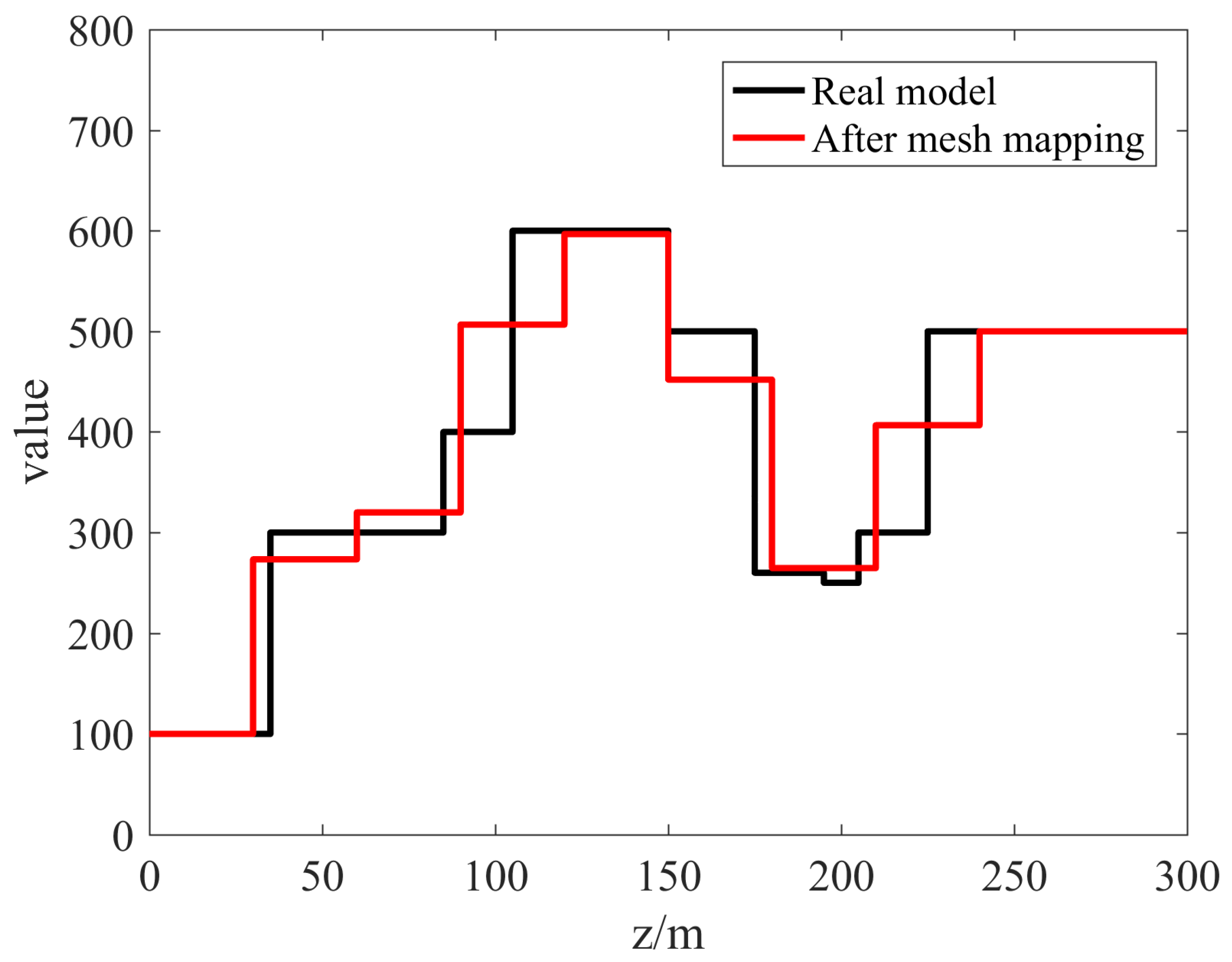
The following is an example of a layered model. Assuming that the original model had 10 layers of media, mesh mapping was used to transform it into a 30 m equidistant thickness model. Table 1 shows the model parameters before and after the equivalent replacement. Figure 4 shows a comparison between the original model and the model after mesh mapping.
Figure 4 shows that the model after mesh mapping effectively retained the structural characteristics of the original model, making it possible to impose structural constraints on the same grid division using other geophysical methods in the cooperative inversion.
In probability theory and statistics, we utilize Pearson correlation coefficients to examine the correlation of models before and after mesh mapping to determine the validity of the mesh mapping method. The Pearson correlation coefficient is used to assess the degree of linear connection between two variables [39], making it perfect for determining the correlation between geophysical data [40]. The Pearson correlation coefficient is written as:
p = c o v X , Y σ x σ y = E X Y E X E Y E X 2 E 2 X E Y 2 E 2 Y
where c o v X , Y represents the X and Y covariances, σ x and σ y are the standard deviations, and E X and E Y are the expected values of X and Y , respectively. The Pearson correlation value, which ranges from −1 to 1, indicates the propensity of two sets of linear data to change concurrently. The correlation coefficient tends to be 1 or −1 when the linear relationship between the two variables is strengthened. When one variable rises and the other rises, there is a positive connection, and the correlation coefficient is larger than 0. If one variable grows while the other falls, the correlation is less than zero. A correlation value of 0 indicates that there is no linear relationship between the two variables.
We sampled the model before and after the mesh mapping with 1 m intervals to obtain the values of each depth within 300 m, and then we analyzed the correlation. We calculated the Pearson correlation coefficient using Equation (15):
p = x i x ¯ y i y ¯ x x ¯ 2 y y ¯ 2 = 0.9237
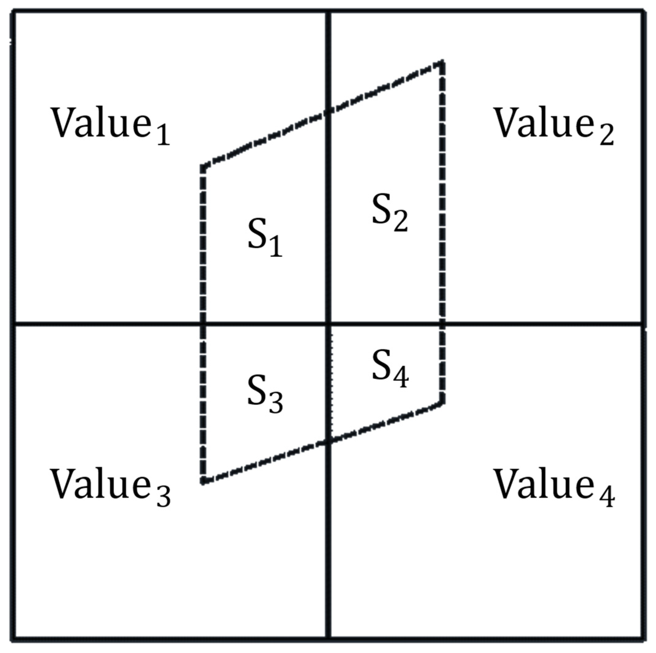
The Pearson coefficient between the model parameters before and after the mesh mapping was 0.9237, which is very close to one, indicating a high linear connection between the two models. This also demonstrates that the mesh mapping method proposed in this study may transform the model parameters between grids of different sizes while preserving the underground structure’s characteristics. This mesh mapping method can also be applied to the cooperative inversion of geophysical methods in high dimensions with disparate grid scales. As illustrated in Figure 5, the two-dimensional mesh mapping method can compute a weighted average of the area. The solid rectangular box represents the initial grid, whereas the dotted box represents the mapped grid. The following formula can be used to calculate the values of each grid after mapping:
v a l u e n e w = i = 1 N S i * v a l u e i i = 1 N S i
A mesh mapping comparison of the two-dimensional model is shown in Figure 6. The initial grid is the unfixed-thickness grid generated by the inversion of the ATEM. To transfer this two-dimensional section to a fixed grid, we employed the mesh mapping method. The structure and morphological characteristics of the underground medium can be preserved after the mesh mapping with minimal distortion. This demonstrates that this mesh mapping method can effectively transition between disparate grid scales, allowing for cross-scale cooperative inversion. The volume weighted average of the underground target grid can complete the mesh mapping at any scale in the three-dimensional example.
To quantify the influence of the mesh mapping approach in the two-dimensional scenario, we used cosine similarity to assess the similarity of the models before and after the mesh mapping. In high-dimensional space, cosine similarity is a typical similarity metric that is frequently employed in information retrieval [41] and data mining [42]. Some academics have employed it for picture similarity learning and depth learning in recent years [43]. Cosine similarity, as opposed to Euclid space distance, highlights the directionality of data changes. The basic concept is to employ feature extraction to convert a high-dimensional data volume into vectors and then compute the cosine value between the two vectors. The lower the cosine value between two vectors, the more similar the representative vectors, demonstrating that high-dimensional spatial data are more comparable. For the two vectors x and y , the cosine similarity may be defined as:
c o s θ = i = 1 d x i × y i i = 1 d x i 2 × i = 1 d y i 2
where θ is the angle between x and y . The similarity between these models increases as c o s θ increases.
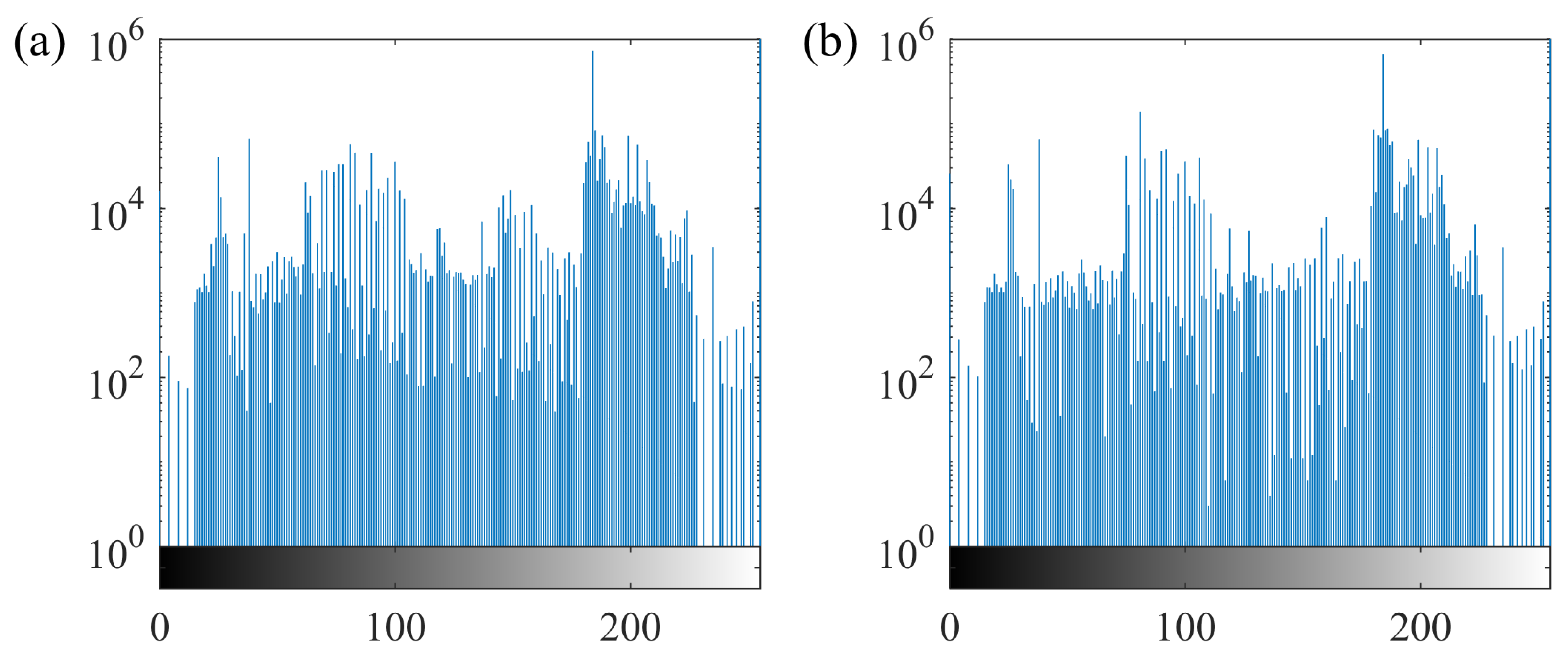
To compare the similarity of the two-dimensional images in this study, the two-dimensional images are first converted into gray images and their corresponding histogram distributions are constructed, as shown in Figure 7. The histogram information is then used to turn the input images into two vectors, and the cosine similarity between the vectors is calculated using Equation (18).
The calculated cosine value was 0.99723, and the vector angle was 4.2663°. This indicates that the model before and after the mesh mapping was remarkably comparable, proving the mesh mapping method proposed in this paper.
In the three-dimensional case, we may use the Monte Carlo method to calculate the volume proportion of the original grid in the new grid, and then utilize the weighted average of the volume method to finish the mesh mapping at any scale, much like in the two-dimensional example.

2.3.3. Cooperative Inversion Strategy

In cooperative inversion, we used cross-gradient constraints to constrain the model structures and the mesh mapping method to integrate various grid sizes. The cross-gradient term was introduced to the objective functions of the ATEM inversion and magnetic inversion, and the two techniques’ constrained inversion was performed iteratively. The objective function is represented by:
Φ A T E M = φ A T E M _ m o d e l + φ A T E M _ d a t a + φ c r o s s
Φ M = φ M _ m o d e l + φ M _ d a t a + φ c r o s s
where Φ A T E M and Φ M are the ATEM and magnetic inversion objective functions, respectively, and this includes the model constraint term φ m o d e l , the data fitting term φ d a t a , and the cross-gradient term φ c r o s s . Using the derivative of the objective function and the iteration formula for inversion:
Δ m A T E M = J T C d J + α C m + β C c 1 J T C m f m 0 d o b s β C c τ c
Δ m M = J T C d J + α C z m + β C c 1 J T C z m f m 0 d o b s β C c τ c
where τ c is the cross-gradient term, C c is the sensitivity matrix derived by taking the derivative of the cross-gradient term with respect to the model parameters, and the derivative matrix of the cross-gradient term is calculated by converting the derivative into a difference operation. The regularization weighting coefficients are α and β , while all other parameters represented have the same meaning as in traditional inversion.
We updated the inversion model using the iterative formula described above until the fitting requirements were met. The fitting difference between the two geophysical methods was calculated using several methods. Because the ATEM utilizes the lateral constraint, the fitting difference should account for both the data fitting and the lateral constraint fitting. Because the magnetic method only considers the data fitting, the fitting difference calculating method is as follows:
r m s ATEM = || W d d o b s W d F M || 2 + || W m R M || 2 / N s 1 × T N
r m s M = || W d d o b s W d F M || 2 / N s
where M is the number of model parameters, N s is the number of measurement points, T N is the number of model parameters, and the other parameters have the same meanings as in Section 2.1 and Section 2.2.
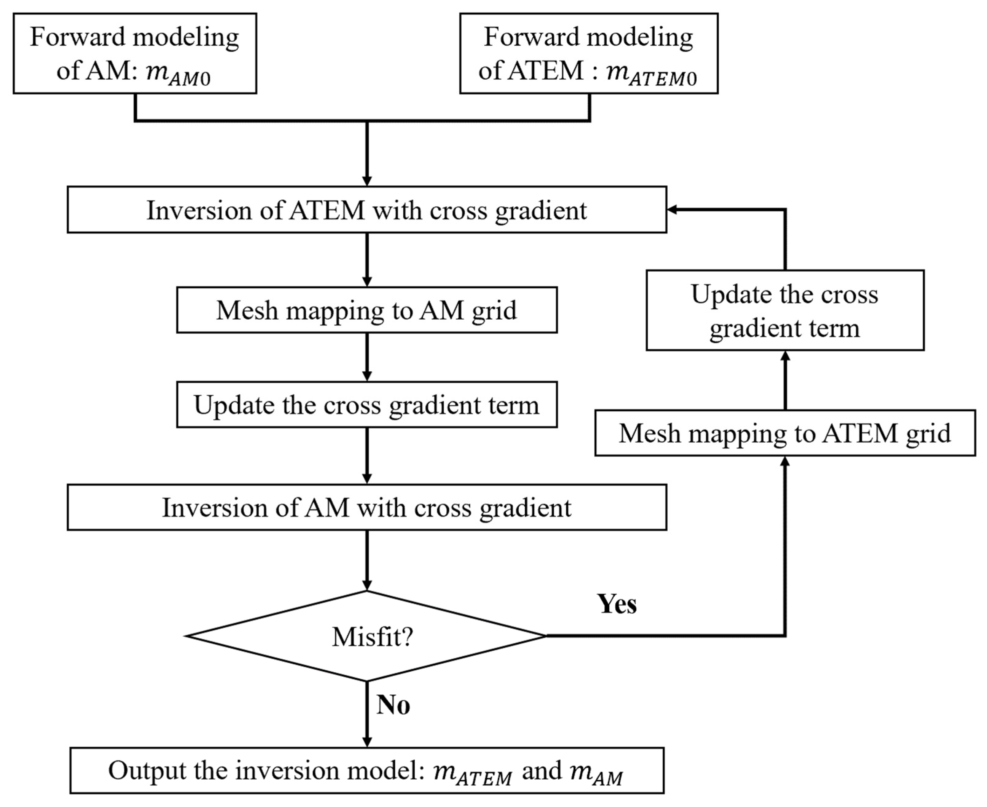
The inversion method is shown in Figure 8. To begin, the initial forward modeling was performed, and the layer thickness and IP parameters were calculated using Equation (21). To enable cross-gradient calculation, the IP model was then transferred to the magnetic grid using the mesh mapping method, and Equation (22) was utilized to complete the magnetic susceptibility update. The magnetic susceptibility model was translated to the ATEM grid after one iteration, and the cross-gradient was updated using the mesh mapping method; the previous iteration processes were continued until the fitting conditions were satisfied.

3. Results

3.1. Model 1 Inversion Results of the Synthetic Data

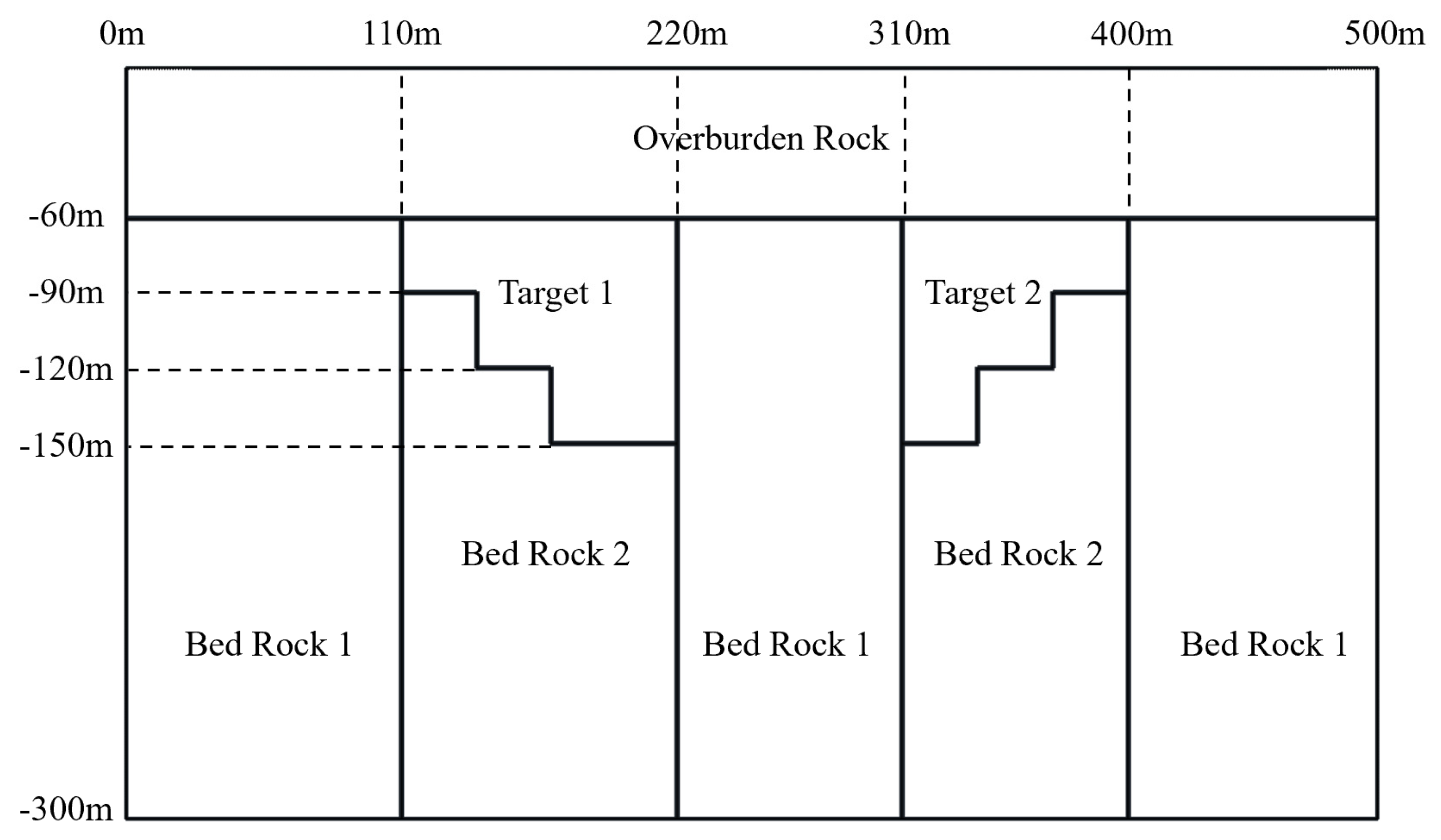
The initial concept proposed in this research was that there were two targets under the 60 m low resistivity overburden, both IP and magnetic, and two types of bedrock beneath. In the model, the intrusive body of igneous rock was represented by the high resistivity body of bedrock 2, and the target body was the ore body. Figure 9 shows the model diagram, and Table 2 shows the individual model parameters.
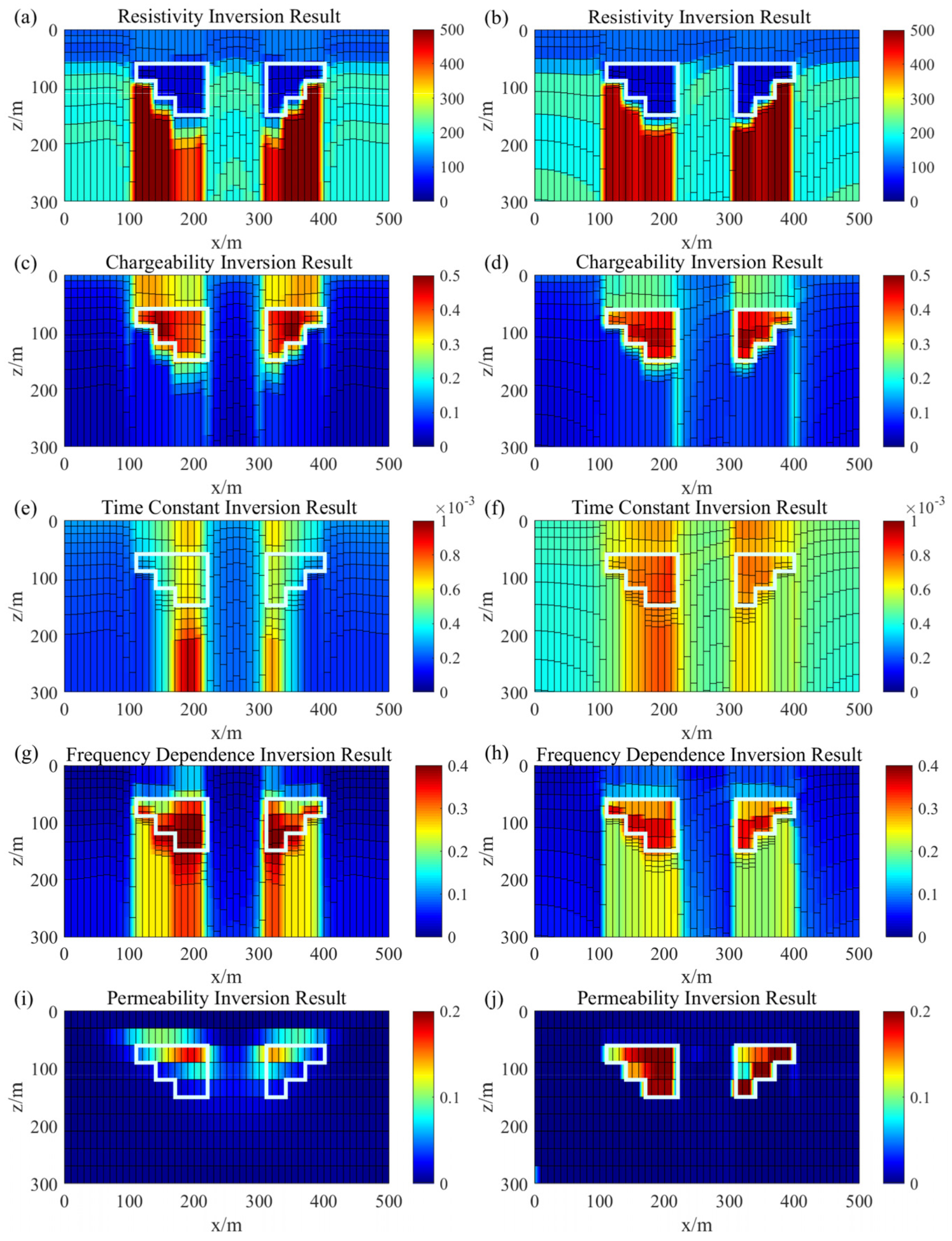
Model 1’s ATEM response and magnetic response were inverted separately and cooperatively. The ATEM’s initial inversion model was a ten layered half-space model with a 15 m initial layer thickness, 100   Ω · m resistivity, 0.1 chargeability, 0.001 time constant, and 0.1 frequency dependency. The initial inversion model of the magnetic method was a homogeneous half-space with a susceptibility equal to 0.1. Figure 10 compares the results.
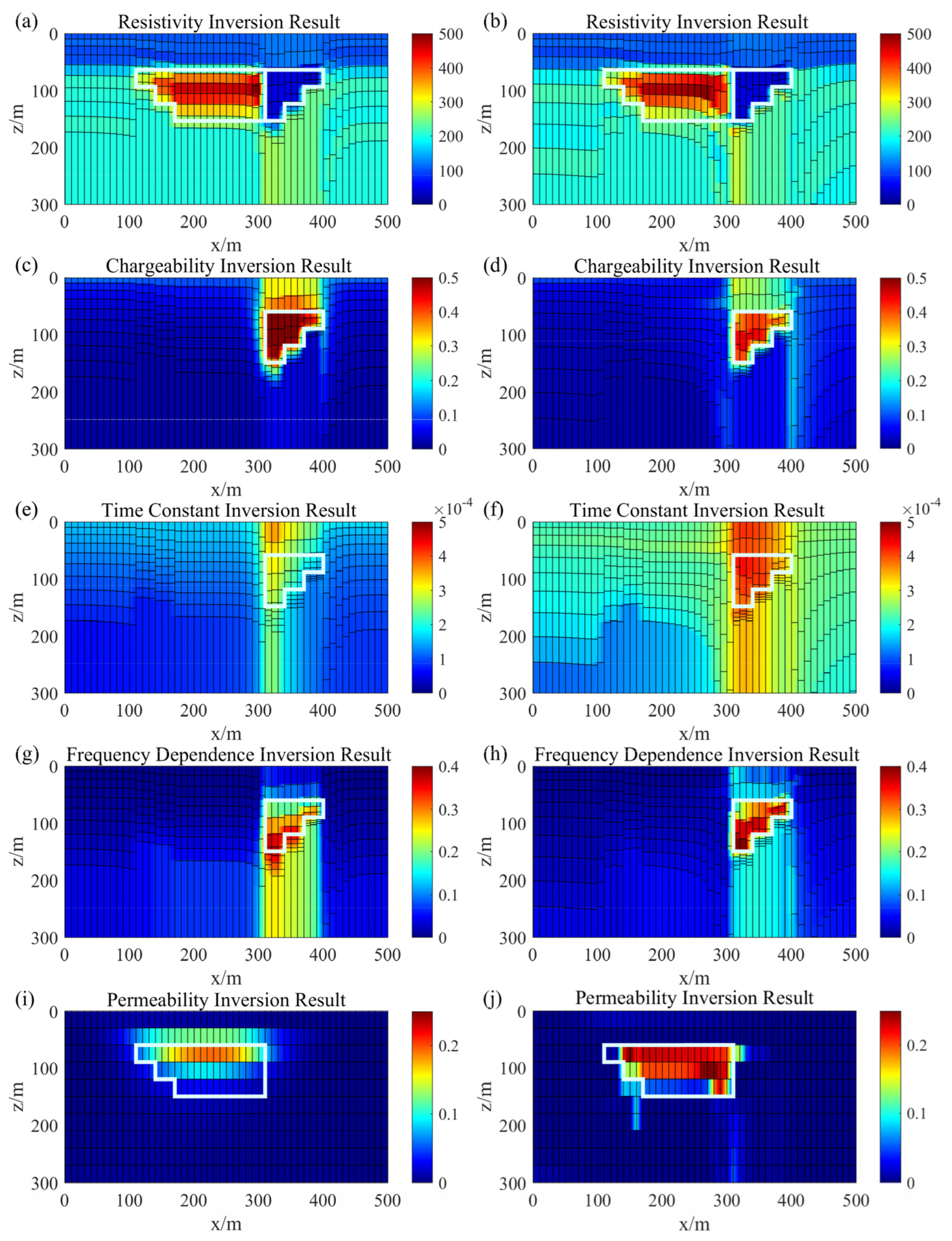
The comparison of the inversion results in Figure 10 shows that imposing cross-gradient structure constraints after mesh mapping improved the inversion results for all physical parameters. Conventional inversion can invert resistivity and chargeability, although it is not ideal for chargeability data. The target’s chargeability was 0.5 in the true model, and the conventional inversion results show a spurious anomaly with a chargeability of 0.3–0.45 above the target; however, the cooperative inversion results effectively fix this problem. The target’s time constant was 0.003. Because this parameter’s sensitivity to the ATEM forward modeling was relatively low, the inversion result was quite poor. After adding structural constraints, the position of the induced polarization body could be recovered better, although there were still some gaps with the true model. The true model had a frequency dependence of 0.3, the parameter value of the target body in the conventional inversion was approximately 0.4, and there was a false anomaly with a value of 0.3–0.4 at the lower half of the target body. However, the cooperative inversion could bring the target body’s frequency correlation coefficient closer to the true value, hence limiting the false anomaly below the target body. The true model susceptibility of the magnetic body was 0.2. Conventional inversion can show the approximate location of a geological body, but the vertical resolution is poor, the boundary division is nebulous, and the inversion result of the target body susceptibility is small, approximately 0.15. Not only can the vertical resolution be significantly improved by adding structural limitations, but the boundary characteristics of the magnetic body can also be clearly displayed, and the value of the magnetic target body can be well restored.
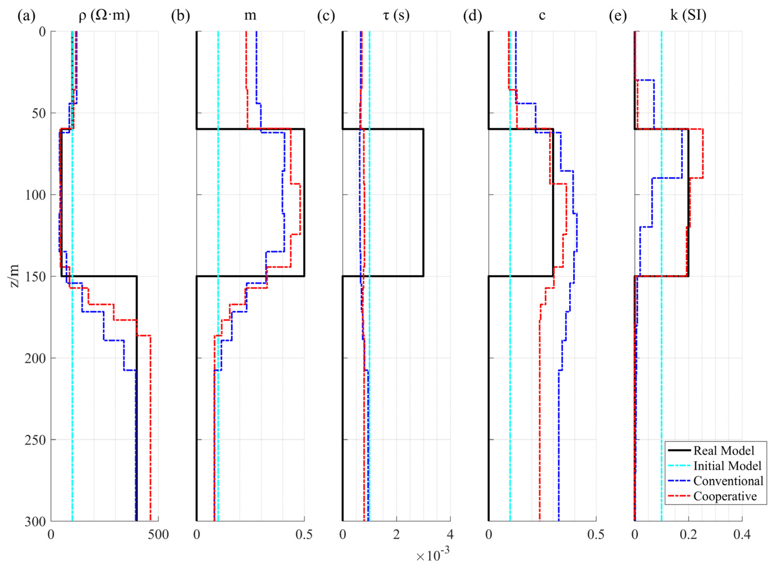
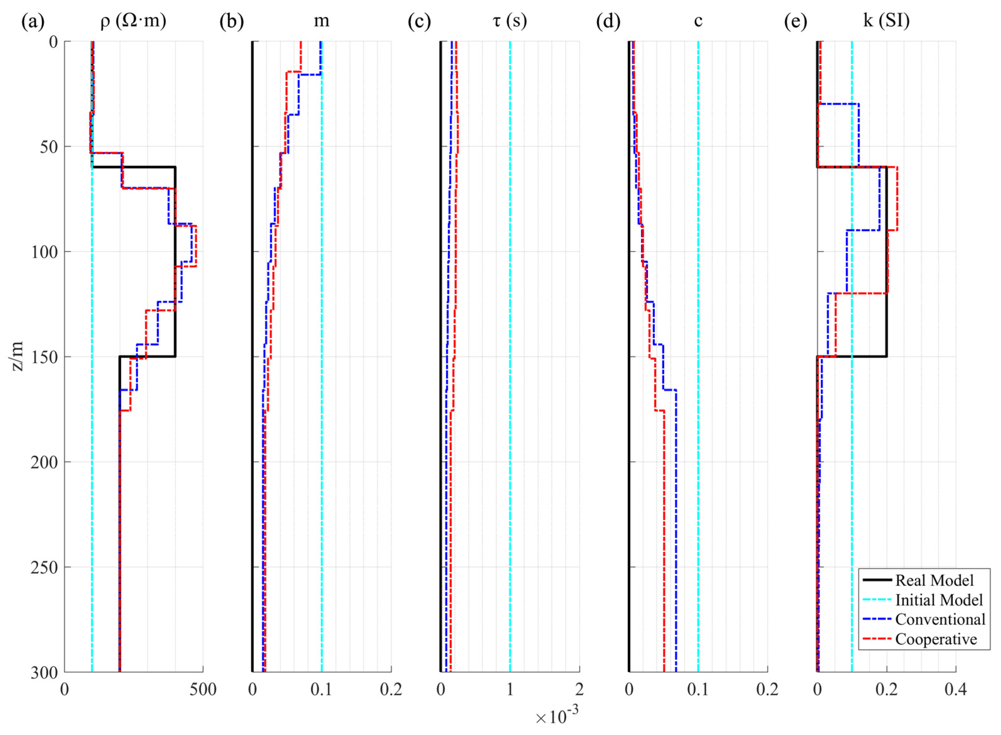
Figure 11 shows the vertical inversion results of the model at 200 m. Based on the one-dimensional inversion results, we can easily compare the improvement of the inversion results using the inversion strategy in this research. The black, solid line represents the true model; the cyan lines represent the initial inversion models, which were all homogeneous half-space models; the blue line represents the result of the traditional inversion; and the red line represents the inversion results of the inversion strategy described in this paper. The cooperative inversion strategy presented in this paper improves the inversion results of the IP and magnetic parameters of rocks to a limited degree, brings the inversion values closer to the true model, and improves the accuracy of the target body position in the inversion results.
Figure 12 shows the convergence of the data from the conventional inversion and the cooperative inversion in terms of the root mean square error. Because more constraints are enforced during cooperative inversion, the number of iterations is greater than in conventional inversion, although it is preferable to exchange a few iterations for improved inversion accuracy. Figure 12c shows the change in the cross-gradient value as the number of iterations increased. The cross-gradient value increased early in the iterations because the model changed dramatically and was far from ideal. When identical models are calculated during the iteration, the value of the cross-gradient decreases, reflecting the role of structural constraints at the late stage of iteration.

3.2. Model 2 Inversion Results of the Synthetic Data

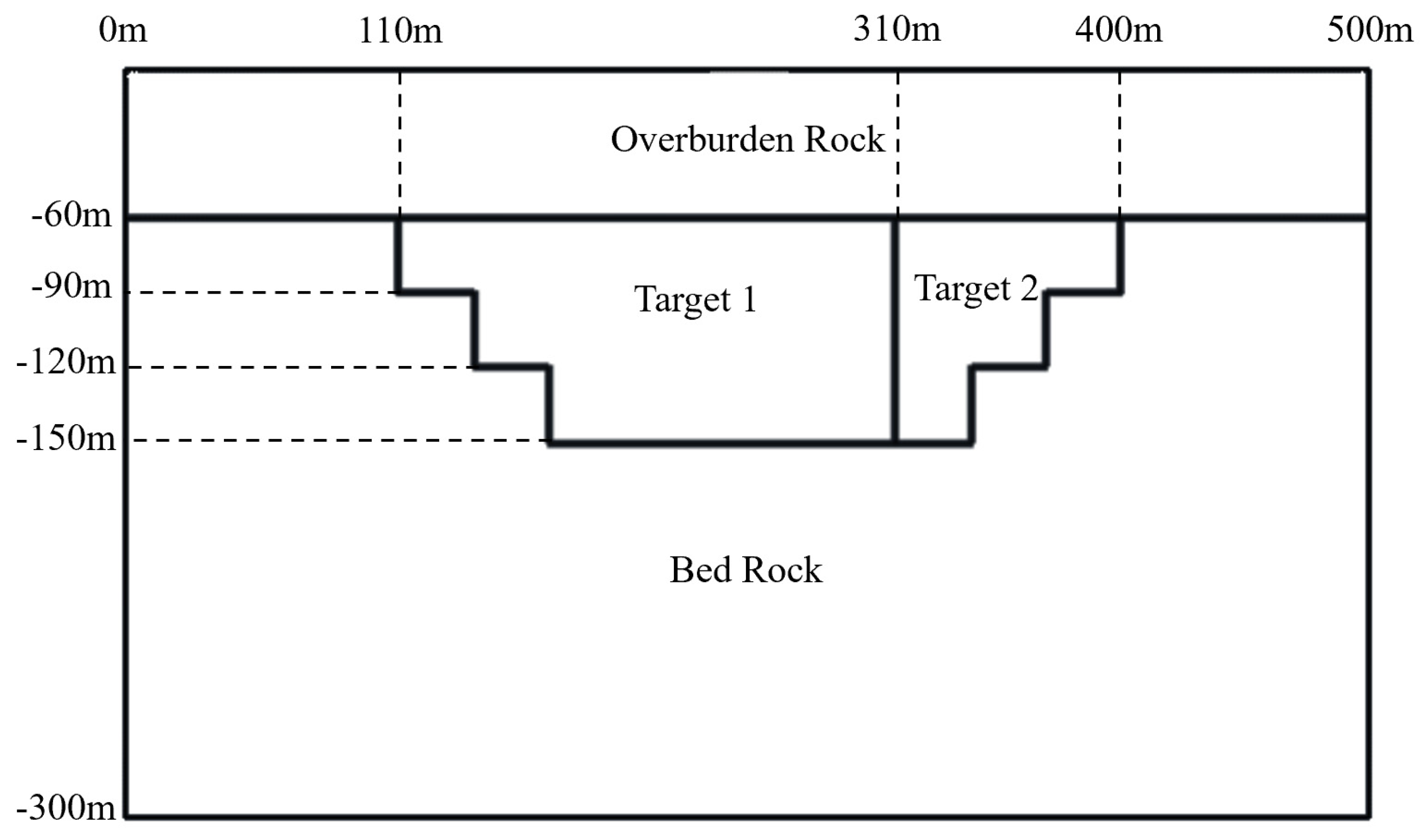
A combined model of the IP and magnetic body was designed for testing in order to prove the method’s universality. Figure 13 shows the model, while Table 3 depicts the specific model lithology characteristics.
The same initial model was chosen for the comparison between the conventional inversion and the cooperative inversion, as with Model 1. The inversion results are shown in Figure 14. This inversion strategy can also better restore the underground IP structure and magnetic structure in the more complex composite model of the magnetic body and IP body.
The inversion results of the chargeability, time constant, and frequency dependency parameters representing the IP parameters can be considerably improved based on the inversion results. The false anomaly with the chargeability of 0.3–0.45 above the target can be effectively suppressed in the inversion results, and the inversion results of the time constant can roughly reflect the location of the IP body, but there was still a significant difference with the true model values. The frequency dependency inversion result and the erroneous anomaly with a value of 0.2–0.3 below can also be efficiently removed. The magnetic body inversion results were also substantially improved, as were the description of the border and the resolution of the depth direction. However, due to the model’s high complexity, there was still a gap between the cooperative inversion results and the theoretical model.
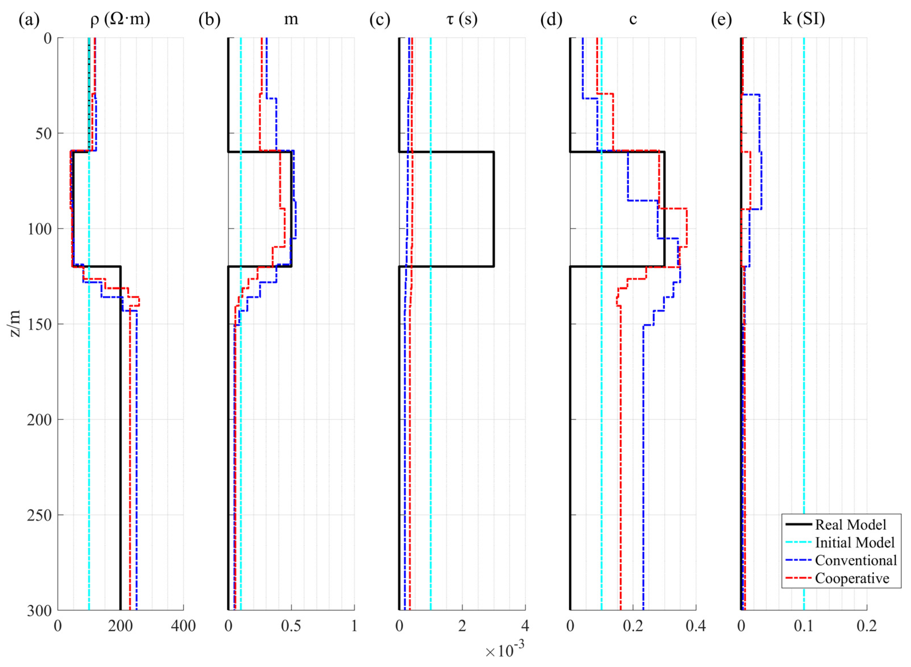
Because the model had two targets, we provided the 1D profile inversion results for the positions of the two targets. The target is an IP body at 200 m and a magnetic body at 350 m. Figure 15 shows how the inversion used in this study increased the magnetic susceptibility inversion results. Figure 16 shows that the chargeability and time constant inversion results greatly improved. Furthermore, due to the impact of the cross-gradient, the susceptibility inversion results produced several erroneous anomalies. When compared to the traditional inversion, the value of the susceptibility remained lower, which is more consistent with the true model. These results demonstrate that the cooperative inversion method utilized in this research may successfully invert the integrated models of various geological targets.

4. Discussion

In this research, we suggested a mesh mapping-based cooperative inversion mechanism. The mesh mapping approach can perform data equivalent replacement at multiple grid partition scales, preserving the original structure of the data better, and it is paired with the structural constraints of the model to perform cooperative inversion under different grids.
First, we used a simple model to demonstrate the effectiveness of the mesh mapping method in 1D and 2D cases, and then we illustrated the idea of the mesh mapping method in 3D. Second, we designed a theoretical model and performed cooperative inversion on its synthetic data to verify the method’s effectiveness.
To perform the cooperative inversion experiments on the synthetic data, the quasi-two-dimensional ATEM with IP effect and the two-dimensional magnetic method were utilized. Multiparameter cooperative inversion yields good results in characterizing the IP and magnetic properties of underground media at the same time. Furthermore, the strategy used in this paper can be extended to the cooperative inversion between geophysical exploration methods at different grid scales.

5. Conclusions

In cooperative inversion, structural constraints are frequently applied. However, because different geophysical methods employ different meshes, several commonly used structural constraint methods cannot be used in the situation of mesh size mismatch. This paper’s mesh mapping approach can translate data between grids of different scales, allowing for the cooperative inversion of mesh mismatches. The examples in this study further demonstrate that the mesh mapping method is particularly well suited to cross-dimensional cooperative inversion.

Author Contributions

Conceptualization, H.R.; methodology, H.R.; software, H.R.; validation, D.L.; formal analysis, D.L.; investigation, H.R.; resources, D.L.; data curation, C.F.; writing—original draft preparation, H.R.; writing—review and editing, D.L.; visualization, H.R.; supervision, Z.W.; project administration, Z.W.; funding acquisition, Z.W. All authors have read and agreed to the published version of the manuscript.

Funding

This work was funded by the Strategic Priority Research Program of the Chinese Academy of Sciences (XDA14050100), the Beijing Science and Technology Plan “Deep Earth Exploration Technology Breakthrough” special project of China (Z181100005718001), and the Scientific Instrument Developing Project of the Chinese Academy of Sciences (ZDZBGCH2018006).

Institutional Review Board Statement

This study is unethical and does not include human or animal subjects.

Data Availability Statement

Data associated with this research are available and can be obtained by contacting the corresponding author.

Conflicts of Interest

The authors declare no conflict of interest.

References

  1. Moorkamp, M. Integrating Electromagnetic Data with Other Geophysical Observations for Enhanced Imaging of the Earth: A Tutorial and Review. Surv. Geophys. 2017, 38, 935–962. [Google Scholar] [CrossRef] [Green Version]
  2. Vozoff, K.; Jupp, D.L.B. Joint Inversion of Geophysical Data. Geophys. J. Int. 1975, 42, 977–991. [Google Scholar] [CrossRef] [Green Version]
  3. Sasaki, Y. Two-dimensional joint inversion of magnetotelluric and dipole data. In SEG Technical Program Expanded Abstracts 1986; SEG: Houston, TX, USA, 1986; pp. 55–57. [Google Scholar]
  4. Maxwell, A.; Meju. Joint inversion of TEM and distorted MT soundings: Some effective practical considerations. Geophysics 1996, 61, 56–65. [Google Scholar] [CrossRef]
  5. Hering, A.; Misiek, R.; Gyulai, A.; Ormos, T.; Dresen, L. A joint inversion algorithm to process geoelectric and sutface wave seismic data. Part I: Basic ideas1. Geophys. Prospect. 1995, 43, 135–156. [Google Scholar] [CrossRef]
  6. Commer, M.; Newman, G.A. Three-dimensional controlled-source electromagnetic and magnetotelluric joint inversion. Geophys. J. Int. 2009, 178, 1305–1316. [Google Scholar] [CrossRef] [Green Version]
  7. Moorkamp, M.; Heincke, B.; Jegen, M.; Hobbs, R.W.; Roberts, A.W. Joint Inversion in Hydrocarbon Exploration; John Wiley & Sons, Inc.: Hoboken, NJ, USA, 2016; pp. 167–189. [Google Scholar]
  8. Lines, L.R.; Schultz, A.K.; Treitel, S. Cooperative inversion of geophysical data. Geophysics 1988, 53, 8–20. [Google Scholar] [CrossRef]
  9. Paasche, H.; Tronicke, J. Cooperative inversion of 2D geophysical data sets: A zonal approach based on fuzzy c-means cluster analysis. Geophysics 2007, 72, A35–A39. [Google Scholar] [CrossRef]
  10. Mcmillan, M.S.; Oldenburg, D.W. Cooperative constrained inversion of multiple electromagnetic data sets. Geophysics 2014, 79, B173–B185. [Google Scholar] [CrossRef] [Green Version]
  11. Zhdanov, M.S.; Jorgensen, M.; Cox, L. Advanced Methods of Joint Inversion of Multiphysics Data for Mineral Exploration. Geosciences 2021, 11, 262. [Google Scholar] [CrossRef]
  12. Archie, G.E. The electrical resistivity log as an aid in determining some reservoir characteristics. Trans. Aime 1942, 146, 54–62. [Google Scholar] [CrossRef]
  13. Faust, L.Y. A Velocity Function Incluing Lithologic Variation. Geophysics 1953, 18, 271–288. [Google Scholar] [CrossRef]
  14. Gao, G.; Abubakar, A.; Habashy, T.M. Joint petrophysical inversion of electromagnetic and full-waveform seismic data. Geophysics 2012, 77, WA3–WA18. [Google Scholar] [CrossRef]
  15. Jegen, M.D.; Hobbs, R.W.; Tarits, P.; Chave, A. Joint inversion of marine magnetotelluric and gravity data incorporating seismic constraints: Preliminary results of sub-basalt imaging off the Faroe Shelf. Earth Planet. Sci. Lett. 2009, 282, 47–55. [Google Scholar] [CrossRef]
  16. Haber, E.; Oldenburg, D.W. Joint inversion: A structural approach. Inverse Probl. 1997, 13, 63. [Google Scholar] [CrossRef]
  17. Gallardo, L.A.; Meju, M.A. Characterization of heterogeneous near-surface materials by joint 2D inversion of dc resistivity and seismic data. Geophys. Res. Lett. 2003, 30, 1658. [Google Scholar] [CrossRef]
  18. Molodtsov, D.M.; Troyan, V.N.; Roslov, Y.V.; Zerilli, A. Joint inversion of seismic traveltimes and magnetotelluric data with a directed structural constraint. Geophys. Prospect. 2013, 61, 1218–1228. [Google Scholar] [CrossRef]
  19. Gallardo, L.A.; Meju, M.A. Joint two-dimensional cross-gradient imaging of seismic traveltime data for structural and lithological classification. Geophys. J. Int. 2007, 169, 1261–1272. [Google Scholar] [CrossRef] [Green Version]
  20. Pak, Y.-C.; Li, T.; Kim, G.-S. 2D data-space cross-gradient joint inversion of MT, gravity and magnetic data. J. Appl. Geophys. 2017, 143, 212–222. [Google Scholar] [CrossRef]
  21. Varfinezhad, R.; Oskooi, B.; Fedi, M. Joint Inversion of DC Resistivity and Magnetic Data, Constrained by Cross Gradients, Compactness and Depth Weighting. Pure Appl. Geophys. 2020, 177, 4325–4343. [Google Scholar] [CrossRef]
  22. Sudha; Tezkan, B.; Siemon, B. Appraisal of a new 1D weighted joint inversion of ground based and helicopter-borne electromagnetic data. Geophys. Prospect. 2014, 62, 597–614. [Google Scholar] [CrossRef]
  23. Carter, S.; Xie, X.; Zhou, L.; Yan, L. Hybrid Monte Carlo 1-D joint inversion of LOTEM and MT. J. Appl. Geophys. 2021, 194, 104424. [Google Scholar] [CrossRef]
  24. Giraud, J.; Seillé, H.; Lindsay, M.D.; Visser, G.; Ogarko, V.; Jessell, M.W. Utilisation of probabilistic MT inversions to constrain magnetic data inversion: Proof-of-concept and field application. Solid Earth Discuss. 2021, 2021, 1–33. [Google Scholar] [CrossRef]
  25. He, H.; Li, T.; Zhang, R. Joint Inversion of 3D Gravity and Magnetic Data under Undulating Terrain Based on Combined Hexahedral Grid. Remote Sens. 2022, 14, 4651. [Google Scholar] [CrossRef]
  26. Spies, B.R. A Field Occurrence of Sign Reversals with the Transient Electromagnetic method. Geophys. Prospect. 1980, 28, 620–632. [Google Scholar] [CrossRef]
  27. Smith, R.S.; Klein, J. A special circumstance of airborne induced-polarization measurements. Geophysics 1996, 61, 66–73. [Google Scholar] [CrossRef]
  28. Cole, K.S.; Cole, R.H. Dispersion and Absorption in Dielectrics I. Alternating Current Characteristics. J. Chem. Phys. 1941, 9, 341–351. [Google Scholar] [CrossRef] [Green Version]
  29. Pelton, W.H.; Ward, S.H.; Hallof, P.G.; Sill, W.R.; Nelson, P.H. Mineral Discrimination and Removal of Inductive Coupling with Multifrequency IP. Geophysics 1978, 43, 588–609. [Google Scholar] [CrossRef]
  30. Auken, E.; Christiansen, A.V. Layered and laterally constrained 2D inversion of resistivity data. Geophysics 2004, 69, 752–761. [Google Scholar] [CrossRef]
  31. Macnae, J. Quantifying Airborne Induced Polarization effects in helicopter time domain electromagnetics. J. Appl. Geophys. 2016, 135, 495–502. [Google Scholar] [CrossRef]
  32. Li, Y.; Oldenburg, D.W. 3-D inversion of magnetic data. Geophysics 1996, 61, 394–408. [Google Scholar] [CrossRef]
  33. Caratori Tontini, F.; Cocchi, L.; Carmisciano, C. Depth-to-the-bottom optimization for magnetic data inversion: Magnetic structure of the Latium volcanic region, Italy. J. Geophys. Res. Solid Earth 2006, 111, B11104. [Google Scholar] [CrossRef]
  34. Nabighian, M.; Corbett, J. Electromagnetic Methods in Applied Geophysics; SEG: Houston, TX, USA, 1988; pp. 203–221. [Google Scholar]
  35. Commer, M.; Newman, G.A. New advances in three-dimensional controlled-source electromagnetic inversion. Geophys. J. Int. 2008, 172, 513–535. [Google Scholar] [CrossRef]
  36. Jupp, D.L.B.; Vozoff, K. Stable Iterative Methods for the Inversion of Geophysical Data. Geophys. J. R. Astron. Soc. 1975, 42, 957–976. [Google Scholar] [CrossRef]
  37. Viezzoli, A.; Kaminski, V.; Fiandaca, G. Modeling induced polarization effects in helicopter time domain electromagnetic data: Synthetic case studies. Geophysics 2017, 82, E31–E50. [Google Scholar] [CrossRef] [Green Version]
  38. Auken, E.; Christiansen, A.V.; Jacobsen, B.H.; Foged, N.; Sørensen, K.I. Piecewise 1D laterally constrained inversion of resistivity data. Geophys. Prospect. 2005, 53, 497–506. [Google Scholar] [CrossRef]
  39. Benesty, J.; Chen, J.; Huang, Y.; Cohen, I. Pearson Correlation Coefficient. In Noise Reduction in Speech Processing; Cohen, I., Huang, Y., Chen, J., Benesty, J., Eds.; Springer: Berlin/Heidelberg, Germany, 2009; pp. 1–4. [Google Scholar]
  40. ChangChun, Y.I.N.; SiYuan, S.U.N.; XiuHe, G.A.O.; YunHe, L.I.U.; Hui, C. 3D joint inversion of magnetotelluric and gravity data based on local correlation constraints. Chinese J. Geophys. 2018, 61, 358–367. (In Chinese) [Google Scholar] [CrossRef]
  41. Korenius, T.; Laurikkala, J.; Juhola, M. On principal component analysis, cosine and Euclidean measures in information retrieval. Inf. Sci. 2007, 177, 4893–4905. [Google Scholar] [CrossRef]
  42. Chakrabarti, S. Data Mining for Hypertext: A Tutorial Survey. SIGKDD Explor. 2000, 1, 1–11. [Google Scholar] [CrossRef]
  43. Xia, P.; Zhang, L.; Li, F. Learning similarity with cosine similarity ensemble. Inf. Sci. 2015, 307, 39–52. [Google Scholar] [CrossRef]
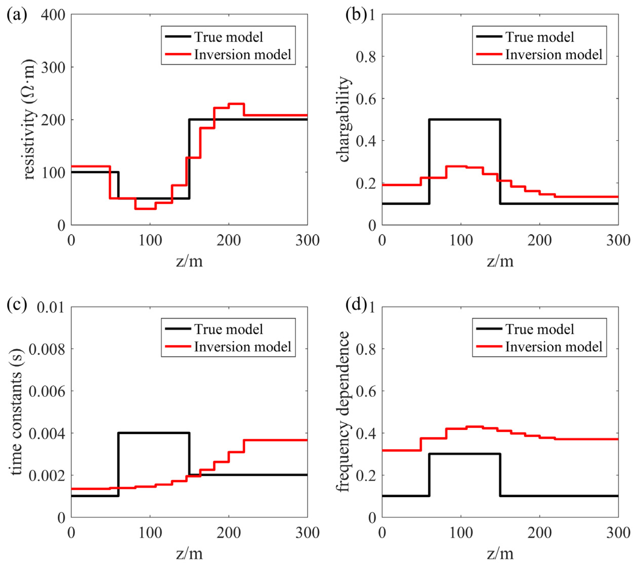
Figure 1. The inversion results of the 1D ATEM: (a) resistivity; (b) chargeability; (c) time constant; (d) frequency dependence.
Remotesensing 15 00125 g001
Figure 2. Diagram of laterally constrained inversion [38].
Remotesensing 15 00125 g002
Figure 3. Schematic diagram of the 1D mesh mapping method.
Remotesensing 15 00125 g003
Figure 4. The comparison between the true model and the model after mesh mapping.
Remotesensing 15 00125 g004
Figure 5. Principle of the 2D mesh mapping method.
Remotesensing 15 00125 g005
Figure 6. Comparison between the models before and after the mesh mapping method in the two-dimensional case: (a) initial model; (b) mesh-mapped model.
Remotesensing 15 00125 g006
Figure 7. Histogram of the gray value: (a) initial model; (b) mesh-mapped model.
Remotesensing 15 00125 g007
Figure 8. Flow diagram of the cooperative inversion method.
Remotesensing 15 00125 g008
Figure 9. Schematic diagram of model 1.
Remotesensing 15 00125 g009
Figure 10. Comparison between the conventional inversion and cooperative inversion results of model 1: (a,c,e,g,i) conventional inversion results; (b,d,f,h,j) cooperative inversion results.
Remotesensing 15 00125 g010
Figure 11. Results of the petrophysical parameters inversion at 200 m: (a) resistivity; (b) chargeability; (c) time constant; (d) frequency dependence; (e) permeability.
Remotesensing 15 00125 g011
Figure 12. Comparison of the data errors between the conventional inversion and cooperative inversion: (a) iterative error of the ATEM inversion; (b) iterative error of the magnetic inversion; (c) cross-gradient value.
Remotesensing 15 00125 g012
Figure 13. Schematic diagram of model 2.
Remotesensing 15 00125 g013
Figure 14. Comparison of model 2’s conventional inversion and cooperative inversion results: (a,c,e,g,i) conventional inversion findings; (b,d,f,h,j) cooperative inversion results.
Remotesensing 15 00125 g014
Figure 15. Results of the petrophysical parameters’ inversion at 200 m: (a) resistivity; (b) chargeability; (c) time constant; (d) frequency dependence; (e) permeability.
Remotesensing 15 00125 g015
Figure 16. Results of the petrophysical parameters’ inversion at 350 m: (a) resistivity; (b) chargeability; (c) time constant; (d) frequency dependence; (e) permeability.
Remotesensing 15 00125 g016
Table 1. Parameters of the original model.
LayerThickness (before)Value (before)Thickness (after)Value (after)
13510030100
22530030273.3
32530030320
42040030506.6
54560030596.6
62550030452
72026030246.6
81025030406.6
92030030500
10-500-500
Table 2. Lithologic parameters of model 1.
Resistivity
( Ω · m )
ChargeabilityTime
Constant
(s)
Frequency
Dependence
Permeability
(SI)
Overburden
Rock
1000000
Target 1500.50.0030.30.2
Target 2500.50.0030.30.2
Bed Rock 12000000
Bed Rock 24000000
Table 3. Lithologic parameters of model 2.
Resistivity
( Ω · m )
ChargeabilityTime
Constant
(s)
Frequency
Dependence
Permeability
(SI)
Overburden
Rock
1000000
Target 14000000.2
Target 2500.50.0030.30
Bed Rock2000000
Disclaimer/Publisher’s Note: The statements, opinions and data contained in all publications are solely those of the individual author(s) and contributor(s) and not of MDPI and/or the editor(s). MDPI and/or the editor(s) disclaim responsibility for any injury to people or property resulting from any ideas, methods, instructions or products referred to in the content.