Article

Combining Different Transformations of Ground Hyperspectral Data with Unmanned Aerial Vehicle (UAV) Images for Anthocyanin Estimation in Tree Peony Leaves

College of Nature Resources and Environment, Northwest A&F University, Yangling 712100, China
*
Author to whom correspondence should be addressed.
Remote Sens. 2022, 14(9), 2271; https://doi.org/10.3390/rs14092271
Submission received: 5 February 2022 / Revised: 26 April 2022 / Accepted: 4 May 2022 / Published: 8 May 2022

Abstract

:
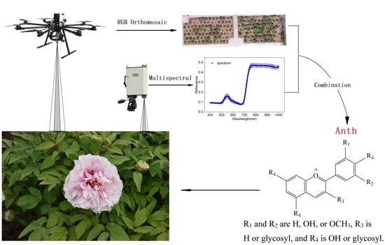
To explore rapid anthocyanin (Anth) detection technology based on remote sensing (RS) in tree peony leaves, we considered 30 species of tree peonies located in Shaanxi Province, China. We used an SVC HR~1024i portable ground object spectrometer and mini-unmanned aerial vehicle (UAV)-borne RS systems to obtain hyperspectral (HS) reflectance and images of canopy leaves. First, we performed principal component analysis (PCA), first-order differential (FD), and continuum removal (CR) transformations on the original ground-based spectra; commonly used spectral parameters were implemented to estimate Anth content using multiple stepwise regression (MSR), partial least squares (PLS), back-propagation neural network (BPNN), and random forest (RF) models. The spectral transformation highlighted the characteristics of spectral curves and improved the relationship between spectral reflectance and Anth, and the RF model based on the FD spectrum portrayed the best estimation accuracy (R2c = 0.91; R2v = 0.51). Then, the RGB (red-green-blue) gray vegetation index (VI) and the texture parameters were constructed using UAV images, and an Anth estimation model was constructed using UAV parameters. Finally, the UAV image was fused with the ground spectral data, and a multisource RS model of Anth estimation was constructed, based on PCA + UAV, FD + UAV, and CR + UAV, using MSR, PLS, BPNN, and RF methods. The RF model based on FD+UAV portrayed the best modeling and verification effect (R2c = 0.93; R2v = 0.76); compared with the FD-RF model, R2c increased only slightly, but R2v increased greatly from 0.51 to 0.76, indicating improved modeling and testing accuracy. The optimal spectral transformation for the Anth estimation of tree peony leaves was obtained, and a high-precision Anth multisource RS model was constructed. Our results can be used for the selection of ground-based HS transformation in future plant Anth estimation, and as a theoretical basis for plant growth monitoring based on ground and UAV multisource RS.

Graphical Abstract

1. Introduction

Anthocyanin (Anth) is one of the three main pigments in plants and is responsible for the color of plant petals and fruits [1]. It is generally found in the cytoplasm of plants and is not a photosynthetic pigment, but can protect the plant’s photosynthetic system from excessive light radiation, especially excessive ultraviolet radiation [2,3]. At the same time, Anth is also a secondary metabolite in plants subjected to environmental and biological stress (e.g., high temperature, water shortage, high salinity, diseases, insects, and pests), and its content can be used as an index to indirectly reflect stress levels [4]. Tree peony, one of the top ten most famous flowers in China, is reputed to be the king of flowers. Its flowers are ornamental, its roots can be used as medicine, and its seeds can be pressed to produce oil; thus, it is a multifunctional plant and has a strong ornamental and economic value. Remote sensing (RS) estimation of Anth content in leaves can not only monitor the health status of tree peonies over time, but also indirectly evaluate their ornamental and economic value [5].
Traditional Anth determination methods are mainly chemical methods, most of which include the extraction of anthocyanins from organic solvents and absorbance analysis by spectrophotometry [6,7]. These methods not only have a long detection cycle, but also involve a complicated process, therefore, have been difficult to popularize in agricultural production. Due to its characteristic multiple bands and narrow bandwidth, hyperspectral (HS) technology can capture fine spectral data of plants and provide rapid, non-destructive, and real-time monitoring of crop growth (e.g., nutrition status, water content, and pest status) [8,9,10,11]. In recent years, scholars have devoted increasing attention to exploring the effects of different spectral transformations on the estimation accuracy of plants’ physiological and biochemical parameters. Shanjun et al. studied the spectral differences of different potato varieties by using the continuous division method [12]. Fenling et al. constructed a hyperspectral model to estimate the nitrogen content of wheat, based on spectral absorption characteristics, determined using the continuum removal method [13]. Zheng et al. obtained the first-order differential, logarithmic, and second-order differential of bamboo leaves, and constructed a principal component analysis-back propagation (PCA-BP) estimation model of bamboo leaves’ nitrogen content, based on three transformed spectra [14]. These studies performed spectral transformation on the original spectrum, eliminated or reduced the influence of bands unrelated to the target properties, enhanced spectral features, expanded the difference between reflected spectral features, and improved the spectral recognition probability, so as to reflect the growth of plants more accurately [15].
Generally, limited by monitoring platforms, the monitoring range of ground-based RS is small, with a high requirement of human and material resources. Therefore, it is difficult to obtain crop growth information on a large scale. Unmanned aerial vehicle (UAV) RS has the characteristics of flexibility, portability, low cost, and wide monitoring range, and can be used as a favorable supplement to ground-based RS. It has become an important technical tool of precision agriculture [16]. The imaging spectrometer carried on the UAV can not only obtain plants’ spectral information, but also their inherent textural and structural information, which are not easily affected by the external environment and can make up for the weakness of easy saturation in the spectral inversion of ground-based RS [17,18]. Scholars have studied nitrogen concentration of cotton and the biomass of wheat by combining RS spectral features with the textural features of UAV images, and the results indicated that the accuracy of the inversion model constructed by the fusion of spectral and texture features was better than that constructed using only texture or spectral features [19,20,21]. However, studies have not yet been reported analyzing biophysical and biochemical parameters closely related to crop growth (e.g., pigment content, nitrogen content, water content, plant height, and leaf area index) using ground-based HS data of different spectral transformations combined with UAV images.
In this study, 30 varieties of tree peony leaves in Shaanxi Province, China, were first determined using a ground spectrometer and UAV RS systems. Second, the three most common spectral transformations were performed on the near-ground spectrum, and Anth estimation models were constructed based on the transformed spectra. Finally, the vegetation index and texture parameters of the UAV images were extracted, and the multi-source RS model of tree peony leaf Anth was constructed, together with the ground spectrum. The purpose of this study was to indirectly monitor tree peony growth on a large scale and with high precision by estimating the level of anthocyanin in peony leaves, thus providing a new idea for monitoring plant growth based on multi-source RS data.

2. Materials and Methods

2.1. Study Area

The experiment was carried out at the tree peony garden of Northwest A&F University in Shaanxi Province, China (34°15′–34°20′N, 107°56′–108°7′E), on 8 April 2018, when the peonies were in full bloom. The average elevation of the garden is 460 m and the climate is warm temperate continental monsoon. There were 32 plots in the study area, among which 2 were mixed variety plots and the remaining 30 were single variety plots. The single variety plots were selected for the study, covering 30 varieties of tree peonies such as Zierqiao, Yinhongqiaopair, and Yaohuang. According to the rule of diagonal sampling, two tree peonies representing the average growth of tree peonies in each plot were selected for spectral and anthocyanin measurement, and a total of 60 peony samples were studied. The location of the study area and the distribution of samples are shown in Figure 1.

2.2. Data Acquisition

2.2.1. Anth Quantification

Leaf Anth was measured with Dualex 4 (FORCE-A, Orsay, France). This measures the leaf epidermal anthocyanin absorbance at 520 nm by means of chlorophyll fluorescence screening, equalizing the chlorophyll fluorescence signal under 520 nm excitation, and that under red excitation at 650 nm, as reported by Goulas et al. [22]. The method also accurately measures the leaf chlorophyll and surface flavonoid contents and nitrogen balance index, and is easy to use for real-time non-destructive measurement. Some scholars have compared Anth measured by traditional chemical methods, such as the Multiplex instrument and UV-A-PAM fluorimeter, with that measured using Dualex, which further proved the reliability of Dualex for Anth measurement [23,24]. To obtain representative Anth, 10 leaves were selected from the tree peony sample, and six Anth measurements were carried out for each leaf, which were then averaged. The measured Anth was subjected to stratified and random sampling at a ratio of 2:1, ignoring the effect of variety; 40 samples were selected for model construction, and the remaining 20 samples were used for model verification. The Anth statistics of the calibration and test sets conducted in our study are shown in Table 1; the data indicated that the Anth content of the calibration set was 0.051–0.171 μg/cm2, and that of the test set was 0.056–0.169 μg/cm2. The test set was within the calibration set and had similar data distribution characteristics to the calibration set. The coefficients of variance (CVs) of the calibration and test sets were 27.722% and 26.732%, respectively, with moderate spatial variation.

2.2.2. Hyperspectral Data Acquisition

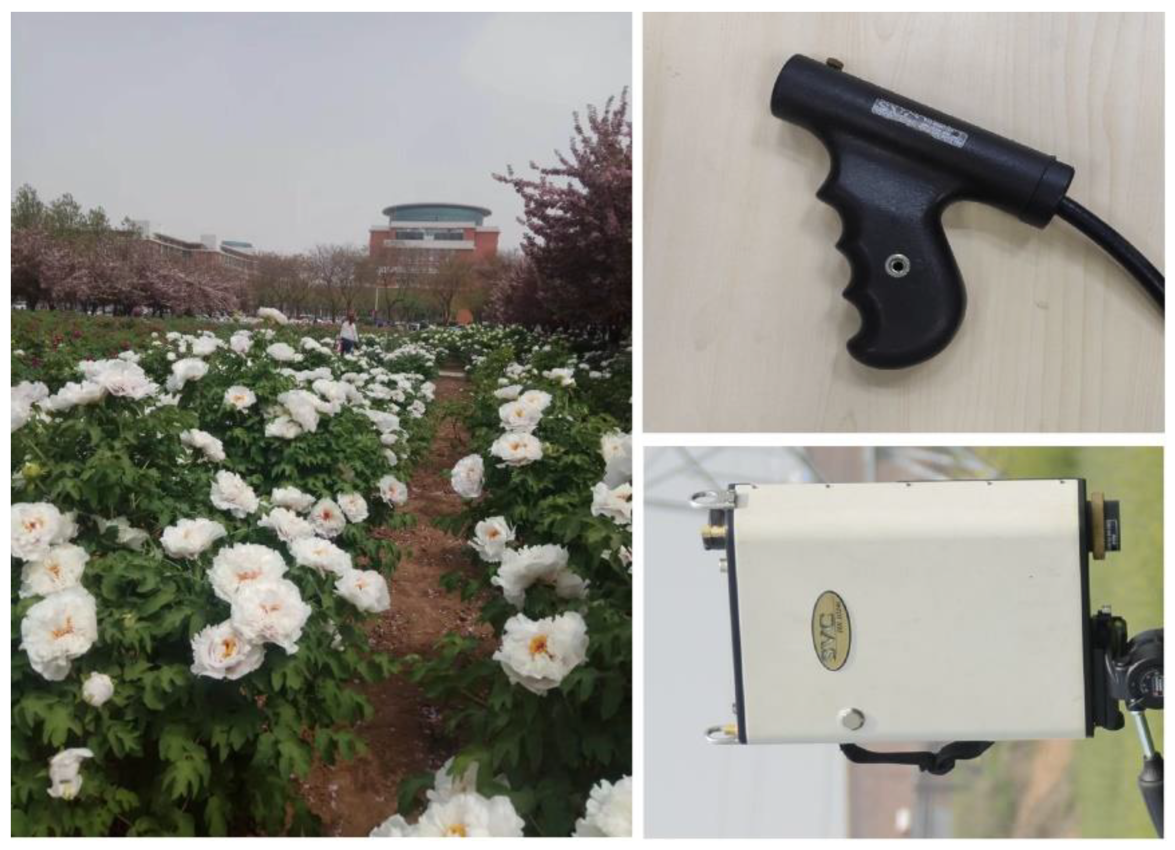
The reflection spectra of tree peony leaves were measured under good weather conditions and stable solar radiation. The instrument used was an SVC HR~1024i spectrometer produced by Spectra Vista Corporation (SVC) of America, with a band range of 350–2500 nm. Firstly, in the absence of any shielding, the test spear head was vertically aligned with the reference plate in the direction of the sun for spectral measurement, and the obtained spectrum was used as a reference for the reflection spectrum correction of the tree peony leaves. Then, the probe connected to the optical fiber (viewing angle of 8°) was placed 30 cm above the tree peony leaves and measured vertically downward. Ten leaves were selected from each tree peony sample, and six spectra were measured for each leaf. Finally, all spectra were averaged as the final spectrum of the tree sample. The spectrometer and tree peony samples are shown in Figure 2.

2.3. Airborne Campaigns

The flight experiment was carried out after the spectral measurement on the ground. The aircraft was Phantom 4 Pro-DJI UAV (DJ-Innovations, Shenzhen, China), which was equipped with a GPS/GLONASS dual positioning module with accurate coordinate information. The weight of the fuselage was approximately 1.4 kg, and the endurance was 30 min under conditions of no wind and maximum load. The aircraft had a built-in dual inertial measurement unit (IMU) and dual compass, which can record its geographical position and three-axis attitude angle in real time during the flight, improving the accuracy of data. The sensor used was the instrument’s 1 inch COM lens, with 20 million effective pixels, 35 mm equivalent focal length, and maximum photo resolution of 19.96 million (5472 × 3648). The flight path was designed in Altizure, with a flight altitude of 50 m, and the flight path overlap rate and side overlap rate were both 75%. Finally, 162 effective RGB (red–green–blue) images were obtained in the experiment.

2.4. Pretreatment and Spectral Transformation of Ground-Based Spectrum

First, the spectrum was preprocessed using Savitzky–Golay filtering in Unscrambler X 10.4 with a smoothing point of 5, while effectively removing the influence of ambient noise. Then the spectral resolution was resampled to 1 nm. The wavelengths that are strongly correlated with plant pigments are concentrated in the visible and infrared regions, and the constituent wavelengths of vegetation indices commonly used for estimating plant physiological and biochemical parameters are also in this region, therefore we studied only the reflection spectra of tree peony leaves in the region of 400–1500 nm.

2.4.1. Principal Component Analysis (PCA) of Spectra

Principal component analysis (PCA) constructs a new orthogonal feature in the K dimension by mapping the original N-dimension feature to the K-dimension (K < N). Only the features containing the most variance were retained, and the features containing almost zero variance were ignored for data dimension reduction [25]. In the field of RS, PCA can effectively remove the correlation, redundancy and collinearity between bands, and is the most widely used method for dimensionality reduction [26]. Therefore, we used this method to reduce the dimension of the tree peony canopy spectrum.

2.4.2. First-Order Differential (FD) Processing of Spectra

First-order differential (FD) processing of plant spectra can compress the influence of background noise on target signals and to a certain extent enhance the contrast of the spectral absorption characteristics of all biochemical components [27]. In this study, the difference method was used to approximate the first-order differential spectrum of peony leaves. The specific calculation formula can be expressed as follows:
R ( λ i ) = R ( λ i + 1 ) R ( λ i 1 ) λ i + 1 λ i 1 10 2
where λi refers to the wavelength of band i, R(λi) refers to the original spectral reflectance corresponding to wavelength λi, and R′(λi) refers to the reflectance of first-order differential spectrum corresponding to wavelength λi.
In the FD spectrum, “three-edge” parameters were the most commonly used spectral parameters, which can accurately reflect the growth status of plants and are the intuitive expression of plant pigment, cell structure, water content, and dry matter quality in the reflection spectrum [28]. We calculated the “three-edge” parameters (position, amplitude, and area) based on the red, blue, and yellow light regions of tree peony leaf reflection spectrum respectively, and their definitions and formulas are shown in Table 2.
Vegetation indices (VIs) based on the FD spectrum have been commonly used to analyze and detect changes in plant physiology and biochemistry [31,32]. These indices, based on information at specific wavelengths, have been developed to reflect diverse plant parameters, such as pigment content, water content, and leaf area. However, the quantitative analysis of a specific tree peony pigment based on the commonly used vegetation indices is not possible at present due the lack of crop species specificity within the available indices. Therefore, to simplify the RS monitoring of tree peony Anth, we constructed differential vegetation index (DVI), ratio vegetation index (RVI), normalized vegetation index (NDVI), and soil-regulated vegetation index (SAVI) for all possible two-band combinations of 400–1500 nm. The coefficients of determination (R2) between Anth and VI can reflect the predictive power of the two independent band combinations.

2.4.3. Continuum Removal Processing of Spectra

Continuum removal (CR), also known as the envelope removal method, was first proposed by Kokaly and Clark [33]. Continuum removal reflectance is the ratio of the original spectral reflectance to the continuum of the corresponding band. The continuum is approximated by a straight line joining the two local reflectance maxima placed on both shoulders (λmin and λmax) of the peak absorption wavelength (λpeak). Continuum removal, CRλ, was thus written as a function of reflectance values R(λ) at wavelength λ, with the constraint that its maximum value could not be above 1.0 (concavity of the reflectance spectra at this location) [34,35].
Continuum removal can effectively remove spectral information noise, eliminate the influence of mesophyll structural parameters, and increase the depth difference of the absorption valley between the spectra of plants with different health statuses. Absorption characteristic parameters based on continuum removal spectrum development can improve the response ability of crop nitrogen and chlorophyll [36,37]. Therefore, in this paper, the seven most commonly used absorption parameters were extracted based on the continuum removal spectrum, and their effect on Anth estimation of tree peonies was investigated. Absorption-band parameters, such as the position, depth, width, and asymmetry of the feature have been used to quantitatively estimate the composition of samples from hyperspectral fields and laboratory reflectance data. In this study, the total area of absorption peak (TA), left area of absorption peak (LA), right area of absorption peak (RA), degree of symmetry (S), normalized maximum absorption depth (NAD), maximum absorption depth (BDmax), and absorption band wavelength (P) were extracted from the CR spectra of tree peony leaves using ENVI 5.1. The definition and calculation formula of the absorption parameters are shown in Table 3.

2.5. Unmanned Aerial Vehicles (UAV) Image Mosaic

2.5.1. RGB (Red-Green-Blue) Gray Vegetation Index Extraction

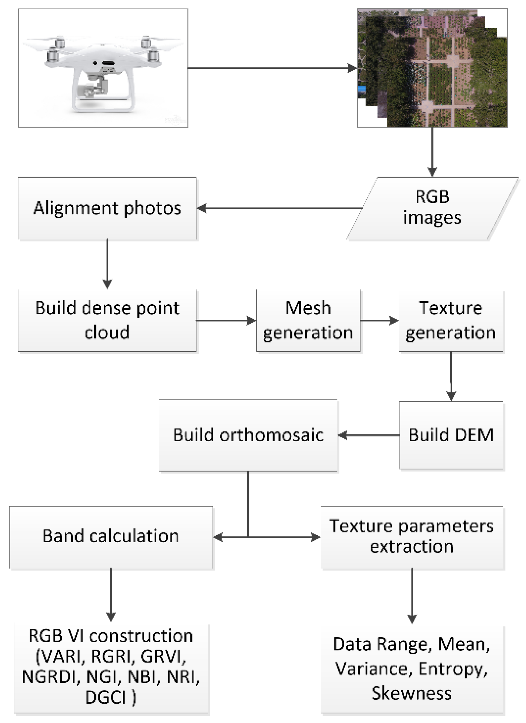
The UAV images were first aligned using the Structure from Motion (SFM) algorithm in the Agisoft PhotoScan professional software (Agisoft, Saint Petersburg, Russia); then, we generated dense point clouds based on the dense multi-view stereo matching algorithm, followed by mesh and texture generation. Finally, an orthomosaic of the study area with real coordinates and detailed texture information was obtained. The mosaic process of the UAV images is shown in Figure 3.
The orthomosaic contained the gray information of the R, G, and B bands, and its pixel size was 0.027 m2 (0.18 m × 0.15 m). Region of interest (ROI) was plotted in ENVI 5.1 to extract the average gray values of the R, G, and B bands of the tree peony sample leaves, and the RGB gray VIs were constructed based on the VI construction principle. Although the gray value was different from the reflectivity of the corresponding wavelength, it was also a quantified expression of the reflected light intensity. Vegetation index is currently extensively used in the field of RS, but most VIs are based on the visible and near infrared bands. However, the sensors in our study were only able to obtain spectral information in the R, G and B bands; therefore, we chose the VIs based on visible light to estimate Anth of tree peony leaves. Among them, the visible atmospherically resistant index (VARI) can highlight the spectral reflection in the visible band, and can reduce the influence of light and atmosphere. The red–green ratio Index (RGRI) was calculated using the ratio of the reflectance of green band and red band. The value of RGRI is closely related to the nutritional status of plants, and has achieved good results in the monitoring of pasture quality and soybean biomass. The normalized green index (NGI), normalized blue index (NBI), and normalized red index (NRI) normalized the reflectance of red, green, and blue bands to a unified standard, and had a good effect on crop recognition. The normalized green–red difference index (NGRDI) was constructed based on the principle of NDVI, making full use of the strong reflection of the green band and strong absorption of red light; it can be used as an alternative to NDVI and has a good relationship with plant growth. The dark green color index (DGCI) was constructed based on the color space of HSV (hue, saturation, value) and represented the greening rate of the plant canopy [41]. Therefore, we constructed the VIs based on gray information from the UAV images, as presented in Table 4.

2.5.2. Texture Parameter Extraction of Unmanned Aerial Vehicle (UAV) Images

In addition to the spectral parameters, the texture characteristics of the image were not easily affected by the color and brightness of the ground objects, and thus, well reflected the growth of plants. Image texture is represented by the gray distribution of the pixel and its surrounding spatial neighborhood. Extraction methods can be divided into structure-based and statistics-based methods. The latter approach was used in this study; statistics-based methods can directly and quantitatively describe the statistical properties of texture features and are increasingly used in plant growth monitoring. The orthographic image of the study area was extracted using texture information based on probability and statistical filtering, and the processing window was 3 × 3. Five texture parameters for the R, G, and B channels were extracted individually, including data range, mean, variance, entropy, and skewness. The UAV image processing flow is shown in Figure 3.

2.6. Regression Model Construction

To explore the influence of modeling methods on model accuracy, multiple stepwise regression (MSR), partial least squares (PLS), back-propagation neural network (BPNN), and random forest (RF) were used to construct Anth estimation models of the tree peony leaves using different transformed spectra. In this study, the predicted residual sum of squares (PRESS) and lowest root mean square error of prediction from cross validation (RMSEPCV) were used to determine the optimal number of LVs and to prevent overfitting. The PRESS statistic determines the number of LVs required to achieve minimum root mean square error (RMSE) between modelled and observed leaf traits. The BPNN used in this study was composed of input, hidden, and output layers. The number of hidden layers of the BPNN model was 1. The number of hidden layer neurons was based on (l: hidden layer neuron, m: input layer neuron, n: output layer neuron, a: constant between 0 and 10), which can constantly adjust the neuron number of the hidden layer to find the model with the highest accuracy. The neuron numbers of both input and output layers were determined by the number of independent and dependent variables. Meanwhile, 10-fold cross verification was used to ensure the stability of the model. The MSR, PLS, and BPNN models were constructed in MATLAB R2016a, and the RF model was constructed in R X64 3.3.3.

2.7. Evaluation Index

The coefficient of determination (R2), root mean square error (RMSE), and relative error of prediction (REP) obtained by unitary linear regression of predicted Anth to measured Anth, were selected as the evaluation index of model accuracy. The closer R2 was to 1, the smaller were the RMSE and REP, indicating the higher accuracy of the model. R2, RMSE, and REP were determined using the following equations:
R 2 = i = 1 n ( y ^ i y ¯ ) 2 / i = 1 n ( y i y ¯ ) 2
R M S E = i = 1 n ( y i y ^ i ) 2 / n
R E P = 100 R M S E y ¯
where yi represents the measured values, y ¯ is the average of the measured value, y ^ i is the predicted value, and n is the number of samples.

3. Results

3.1. Characteristics of Spectrum

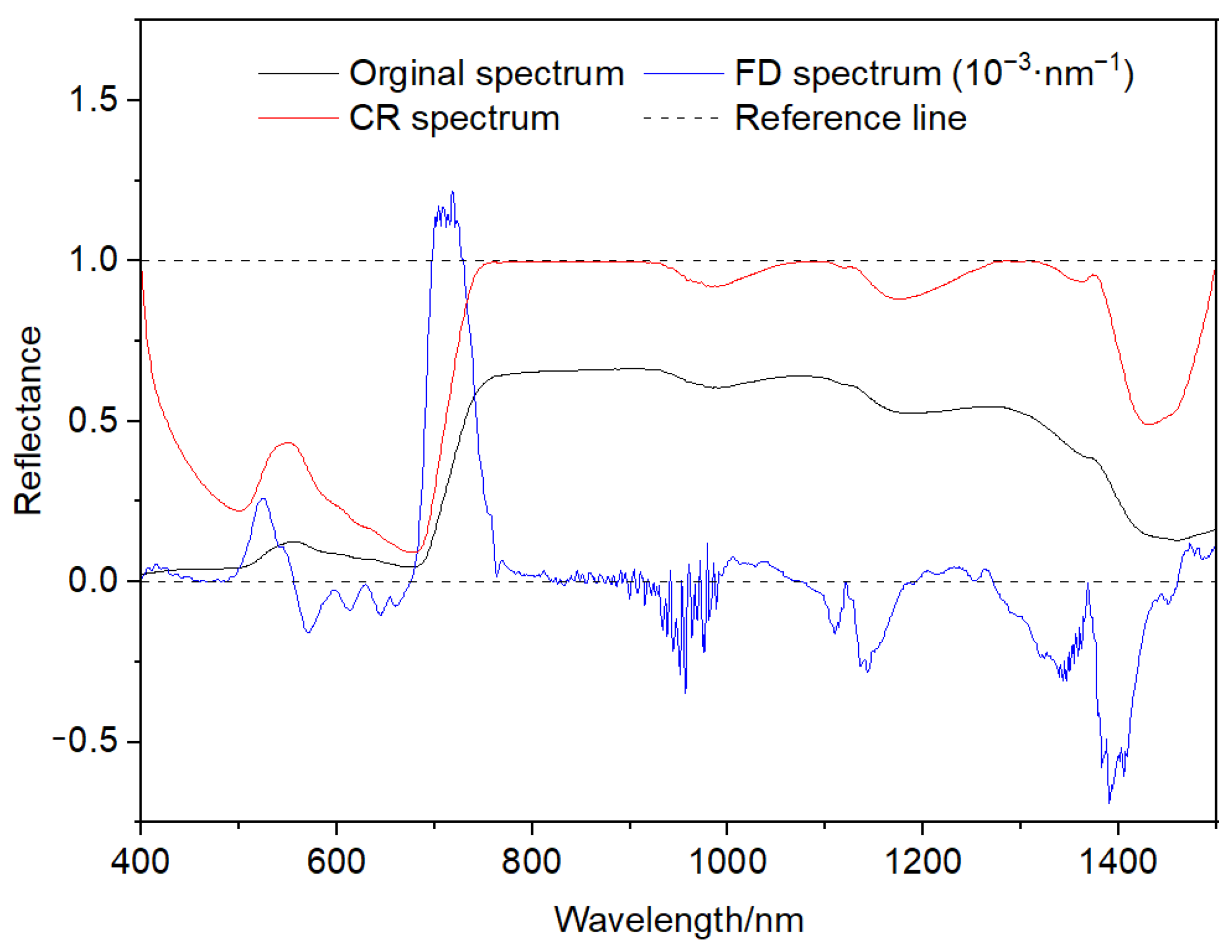
Based on the three spectra of tree peony leaves in Figure 4, it is evident that the CR method projects the original spectral reflectance in the range of 400–1500 nm to 0–1, such that the spectral reflectance in the ranges of 400–747 nm, 932–1056 nm, 1109–1267 nm, and 1324–1500 nm shows more obvious variance. Hence, it can be concluded that the CR spectrum is sensitive to the variation in spectral reflectance. The FD spectral conversion method not only removes the baseline but also avoids excessive signal-to-noise ratio reduction in the corrected spectrum. In this study, the maximum FD spectral reflectance of tree peony leaves appeared at 723 nm, indicating that the original spectral reflectance increased most rapidly in this band. This is a unique spectral characteristic of green plants. The minimum value of FD spectral reflectance appeared at 1405 nm, showing that the original spectral reflectance decreased most rapidly in this band. Noticeably, the FD spectrum was sensitive to the rate of change of the original spectral reflectance.

3.2. Principal Components of PCA Spectrum

According to the principle of initial eigenvalue greater than 1, a total of nine principal component variables were screened out and labeled F1 to F9, respectively; their cumulative variance contribution rate was 99.8 %. The PCA results of tree peony leaves spectra are shown in Figure 5.

3.3. Vegetation Index of Any Two Bands of FD Spectrum

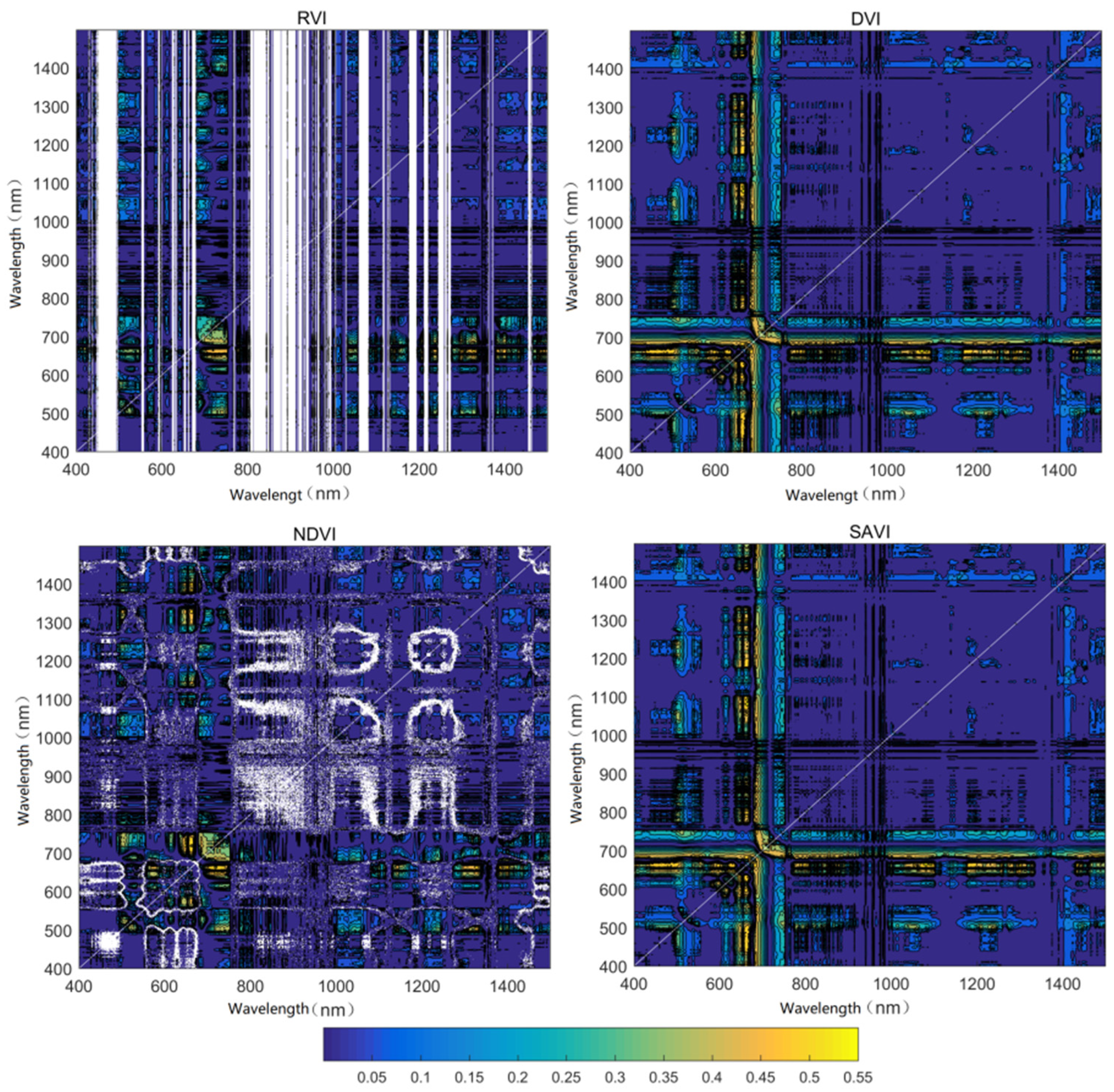
As shown in the contour map of R2 shown in Figure 6, the R2 distribution of DVI and SAVI had obvious similarity, and the distribution of the high value area of R2 was wider than that of RVI and NDVI. The optimal band combinations of RVI, DVI, NDVI and SAVI were (D661 nm, D1475 nm), (D666 nm, D1082 nm), (D664 nm, D720 nm) and (D666 nm, D1082 nm), respectively, and the corresponding maximum R2 was 0.57, 0.48, 0.51 and 0.48, respectively.

3.4. Correlation Analysis between Spectral Parameters and Anth

Table 5 shows the correlation coefficient between Anth of tree peony leaves and the principal components of the PCA spectrum, “three-edge” parameters of the FD spectrum, and absorption parameters of the CR spectrum. It is evident that principal components F1, F2, and F8 were significantly positively correlated with Anth (p < 0.05) while F4 and F5 were significantly negatively correlated with Anth (p < 0.05). The highest correlation was with F8, with the correlation coefficient being 0.37. Meanwhile, F7 and F9 had the worst correlation with Anth. Among the “three-edge” parameters, λr had the best correlation with Anth, the correlation coefficient reaching −0.5, followed by SDb and λy. Overall, position-based parameters (λr and λy) had a higher correlation with Anth than those based on area (Dr and Dy) and amplitude (SDr and SDb).
Taking as the boundary the reflection peaks observed at 550 nm of the green light, CR transformation was carried out at 400–550 nm, 550–788 nm and 400–788 nm. The correlation coefficient between absorption parameters and Anth shows that the correlation between Anth and the absorption parameters at 550–788 nm and 400–788 nm was higher than that at 400–550 nm, and most of the absorption parameters were significantly correlated with Anth (p < 0.05). P at 400–550 nm, NAD at 550–788 nm and RA at 400–788 nm were the absorption parameters with the best correlation with Anth in the corresponding band range.

3.5. Correlation Analysis between Unmanned Aerial Vehicle (UAV) Parameters and Anth

Table 6 shows the correlation between the RGB gray vegetation index, texture parameters and Anth. Only NRI was positively correlated with Anth, and VARI, RGRI, GRVI, NGRDI, and DGCI were all significantly negatively correlated with Anth, with DGCI portraying the highest correlation; the correlation coefficient was −0.6. The mean of the R band had the greatest correlation with Anth, with a correlation coefficient of 0.52, while the mean of the B band had the lowest correlation. Overall, the correlation between the texture parameters and Anth was low.

3.6. Anth Estimation Based on Hyperspectral (HS) of Different Spectral Transformations

The results of the model’s calibration and test sets are shown in Table 7. The R2c of the model based on the PCA spectrum was between 0.45 and 0.91, and the R2v was between 0.21 and 0.58. The R2c of the model based on the FD spectrum ranged from 0.53 to 0.91, and the R2v ranged from 0.51 to 0.59. The model based on the CR spectrum had an R2c range from 0.57 to 0.87, and an R2v range from 0.25 to 0.34. Obviously, there was a large difference in the modeling accuracy with respect to different modeling methods, with a small difference in the test accuracy. Meanwhile, considering R2c and R2v, the accuracy of the FD spectral model was better than that of the PCA and CR spectral models. In the PCA and FD spectral models, compared with MSR and PLS, BPNN and RF were the better modeling methods. The PCA-RF and FD-RF models had the highest R2c, and the PCA-BPNN and FD-BPNN models had the highest R2v. However, both the PCA-RF and FD-RF models experienced over-fitting; this was because the amount of training data was small in this experiment, and the model overfitted the training data without considering the generalization ability. The PLS model portrayed moderate accuracy, while the MSR model portrayed good performance only in the calibration set of the PCA model (R2c = 0.45, R2v = 0.21). This was because both MSR and PLS are linear models, and stable and effective regression can be performed in the presence of multicollinearity of independent variables. However, PLS combines the characteristics of multiple linear regression (MLR), canonical correlation analysis (CCA), and principal component analysis (PCA), and the final model contains the information of all the original independent variables, while the MSR model contains only the information of several important variables [47]. Among the CR spectral models, the accuracy of the test set was low, and overfitting occurred in all of them, which may be because the parameters used in the CR models were extracted based only on the measurements acquired at 400–550, 550–778, and 400–778 nm, and the spectra in these band regions were mainly affected by Chl and less affected by Anth. In general, the FD-RF model had the best calibration accuracy (R2c = 0.91, RMSEc = 0.01, REPc = 10.45%), and the FD-BPNN model had the best test accuracy (R2c = 0.59, RMSEc = 0.04, REPc = 31.23%).

3.7. Anth Estimation Based on Unmanned Aerial Vehicle (UAV) Images

Tree peony Anth estimation models based on UAV VIs and texture parameters were structured in Table 8. The R2c ranged from 0.49 to 0.71, and the R2v ranged from 0.25 to 0.45; the R2c of each model was obviously higher than its R2v. Among them, the UAV-RF model had the highest calibration and test accuracy, R2c and R2v were 0.71 and 0.45, respectively. The UAV-BPNN and UAV-MSR models followed, and the UAV-PLS model had the worst accuracy. This was because the RF model performed regression through repeated binary data, and its sampling method and the generation of decision tree features were random; therefore, the prediction accuracy of the model could be improved without significantly increasing the amount of computation [48]. Compared with the ground-based FD-RF model, the accuracy of the UAV-RF model was low in the calibration and test sets; this is mainly because the ground spectrum had higher spatial resolution and rich band information, and the spectral reflectance obtained of ground objects was more precise than that obtained by the UAV sensor.

3.8. Anth Estimation Based on Multi-Source Remote Sensing (RS) Data

To make full use of the rich band of HS, as well as the flexible, fast, and wide monitoring range of UAVs, the multi-source RS model was constructed by combining the parameters extracted from different ground-based spectra and UAV images (Table 9). The R2c ranges of the models based on PCA + UAV, FD + UAV, and CR + UAV were 0.73–0.92, 0.75–0.93, and 0.61–0.91, and the R2v ranges were 0.34–0.58, 0.65–0.76, and 0.35–0.56, respectively. Obviously, the model based on FD + UAV had the highest accuracy in both the calibration and test sets, and the RF model had the highest accuracy (R2c = 0.93, R2v = 0.76), followed by the BPNN model (R2c = 0.85, R2v = 0.69), whereas the MSR and PLS models had relatively poor accuracy. Among the models based on PCA + UAV and CR + UAV, the modeling accuracy of the RF model was the highest in both the calibration and test sets (R2c = 0.92 and 0.91, respectively), and the verification accuracy of the BPNN model was the highest in both the calibration and test sets (R2v = 0.58 and 0.56, respectively). The accuracies of the MSR and PLS models were obviously lower.
Compared with the PCA, FD, and CR ground-based models, the accuracy of the multi-source RS model improved in both the calibration set and the test set, and the most obvious improvement was in the model based on FD + UAV. With the addition of UAV information, the R2c of the optimal ground-based model increased from 0.91 to 0.93, and R2v increased from 0.51 to 0.76; thus, the RF model of FD + UAV was the best multi-source RS model for tree peony leaves Anth estimation. Compared with the optimal UAV model (UAV-RF), R2c improved from 0.71 to 0.93 and R2v improved from 0.45 to 0.76, and the accuracy of the calibration and test sets improved by 30.99 % and 68.89 %, respectively.
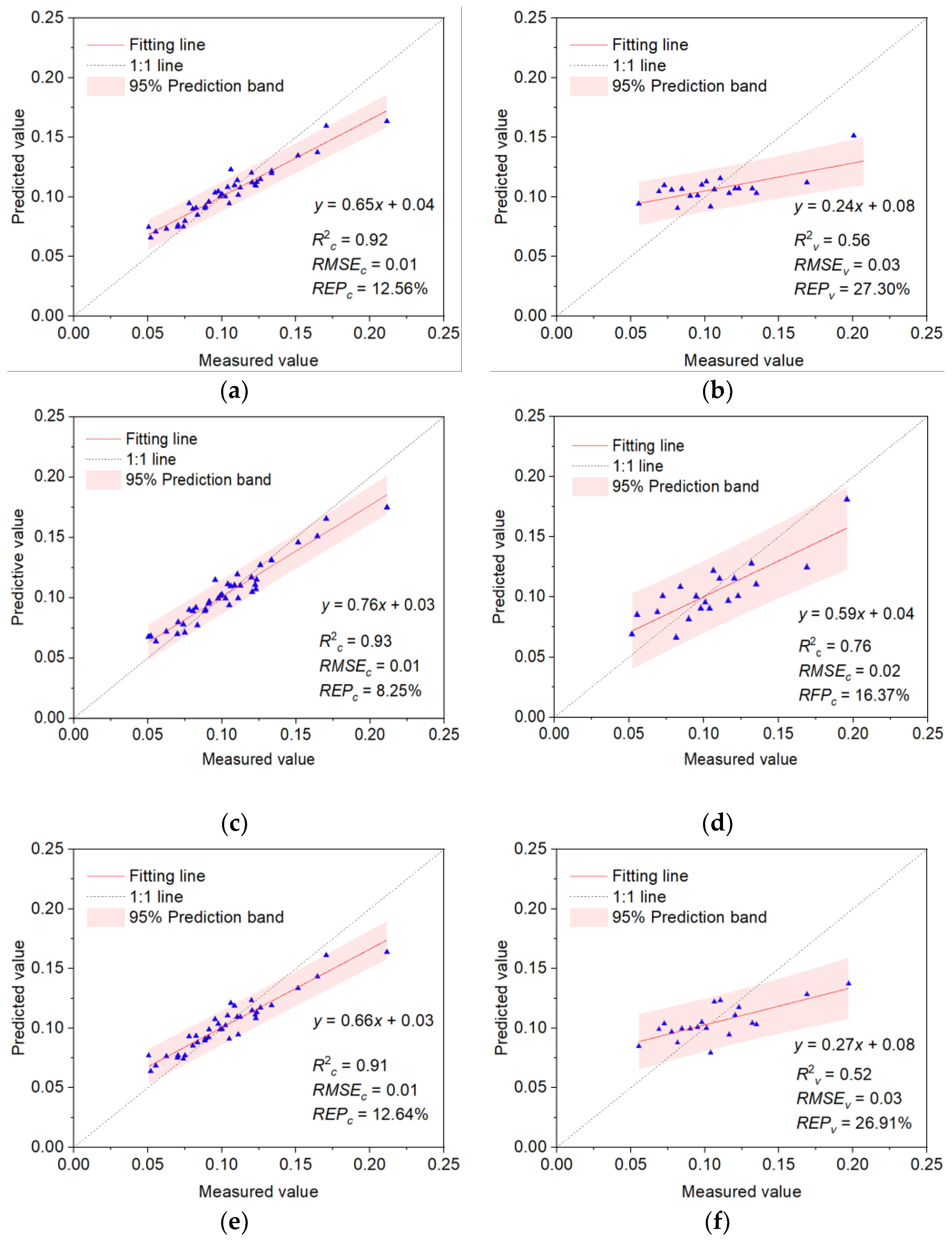
In multisource RS models, the RF model showed an obvious superiority over the BPNN, PLS and MSR methods; the optimal models based on PCA + UAV, FD + UAV, and CR + UAV were all constructed by the RF model. Figure 7 shows the fitting effect of predicted Anth on measured Anth for the RF models; the predicted value of the calibration set had a good fitting effect (R2c is all over 0.9), and the Anth content was evenly distributed on both sides of the 1:1 line, without obvious aggregation. The predicted values of the test set had a slightly poor fitting effect; when the Anth value was near 0.10, the predicted Anth was close to the measured Anth, whereas when the Anth value was far from 0.10, the Anth prediction portrayed a large deviation from the measured Anth. Among all the models, the RF model of FD + UAV had the best fitting relationship between the predicted and measured Anth values in the calibration and test sets.

4. Discussion

4.1. Application of Spectral Information Extraction from Hyperspectral (HS) Data

HS sensors collect information over a very large number of wavelengths, equivalent to dozens or hundreds of wavebands. However, due to the large amount of HS data, not all acquired bands are highly correlated with target features. HS data compression methods can be divided into lossless compression and lossy compression. Lossless compression methods are based on statistical redundancy of suppressed data, whereas a lossy algorithm minimizes the data by discarding irrelevant parts of the information. These methods all de-correlated the HS data to represent the inherent information content in a low-dimensional domain [49]. However, from the perspective of coding gain, PCA was considered to be the optimal transformation of gaussian sources. In this study, PCA was used to compress the 400–1500 nm band region into nine principal component variables, which maximized the information of the original spectrum, while greatly reducing the spectral dimension. Notably, the cumulative variance contribution rate of all principal components was as high as 99.8%, which almost entirely represented the spectral information of tree peony leaves in the whole band region, and effectively extracted the reflection spectrum of tree peony leaves.
Among the techniques developed in spectroscopy, derivative analysis has been particularly promising in the application of RS data [50]. The derivative of the spectrum, its rate of change with respect to the wave length, overcame many of the problems of quantitative analysis in a more elegant and efficient manner by comparing ratios and differences [51]. In the field of RS, FD spectroscopy has mainly been used to help locate critical wavelengths. Guo et al. constructed a high-precision estimation model of chlorophyll content in tobacco leaves by constructing a normalized variable (SDr − SDy)/(SDr + SDy) based on the FD spectrum [52]. In this study, “three-edge” parameters and VI extracted from the FD spectrum portrayed a good correlation with Anth, and the model accuracy based on FD and FD + UAV was better than that based on PCA and the CR spectrum, which fully reflected the superiority of the FD method in spectral transformation research.
CR analysis removes the uninteresting absorption features by dividing the reflectance value of each point using the reflectance of the continuum line (convex lobe) at the corresponding wavelength, thus, standardizing and enhancing the specific absorption characteristics of foliar biochemical components [53]. Among the absorption characteristic parameters extracted based on the CR spectrum, the NAD of 550–788 nm had the strongest correlation with Anth, and the correlation coefficient reached 0.63. However, the models built based on CR and CR + UAV experienced over-fitting, which was related to the narrow band range of extracting absorption characteristic parameters and the fact that the spectrum of these regions was mainly affected by the Chl content and less affected by the Anth content.

4.2. Advantages of Ground-Based Spectrum and Unmanned Aerial Vehicle (UAV) Data

With the rapid development of UAV and lightweight hyperspectral imaging (HSI) sensors, mini-UAV-borne hyperspectral remote sensing systems have been developed, and demonstrate great value and application potential. In this study, UAV multi-spectral information, texture information, and ground HS data were combined to estimate accurately the Anth content of tree peony leaves, by overcoming the saturation problem related to VI in scenarios of dense canopies [54]; variable structural characteristics of the canopy can also be effectively detected using this method [55]. Notably, this method is superior to Anth estimation using ground HS data and UAV images individually. This is consistent with the results of a study conducted by Zheng et al. [56] in which rice nitrogen content was estimated by vegetation index and texture parameters, based on near-ground and UAV platform spectra.

4.3. Machine Learning and Plant Growth Monitoring

Compared with physical radiative transfer models, empirical statistical models have been widely used in the study of plant growth due to their stable, easy-input parameters, and simple modeling methods. Among these, machine learning algorithms can deal with regression problems arising from the complex relationships between independent and dependent variables, while achieving reliable estimations of plant pigment content, nitrogen content, LAI, and biomass [57,58,59,60]. Among the MSR, PLS, BPNN, and RF models constructed in this study, the BPNN and RF models demonstrated obvious superiority, which was consistent with the findings of previous researchers that the RF and BPNN methods had obvious advantages for cotton LAI estimation, citrus pest identification, wetland plant total nitrogen inversion, and winter wheat growth monitoring [61,62,63]. This was because the BPNN model is generally a multilayer feedforward neural network, with signal forward propagation and error back propagation. In this model, the input signals are processed step by step, from the input layer to the output layer, through multiple hidden layers. When the output layer is inconsistent with the desired output, it turns to back propagation, apportioning the error to all the cells in each layer. Error signals are used to correct the weights of each unit, so that the predicted output of BPNN is consistently close to the expected output [64]. The BPNN models in this study all set the hidden layer number to 1, according to newff function, and thus we could develop an optimal training model by constantly changing the hidden layer node number. Finally, the hidden layer nodes of the PCA-BPNN, FD-BPNN, and CR-BPNN optimal models were 6, 8, and 10, respectively, and the hidden layer nodes of the BPNN models based on PCA + UAV, FD + UAV, and CR + UAV were 10, 8, and 9, respectively. With the addition of UAV information, the accuracy of the BPNN model based on multi-source RS data greatly improved compared with the model constructed from single-source RS data. The most obvious improvement was in the model based on CR + UAV, where R2c increased from 0.59 to 0.73 and R2v increased from 0.27 to 0.56. This is consistent with previous findings that the BPNN model has a positive effect on net primary productivity estimation, as shown by Yan et al., and for soil pH study, as reported by Huang et al. [37,65]. The RF model applied an integration algorithm, with high accuracy and generalization ability. It performed regressions through repeated dichotomous data, and the generation of sampling method and decision tree features was random; therefore, we could increase the prediction accuracy significantly, without significantly increasing the amount of computation [66]. In the PCA-RF, FD-RF, and CR-RF models constructed in this study, R2c was greater than 0.85, which was higher than the accuracy of other models constructed on the same spectrum, but its R2v was slightly less than that of other models. Thus, we could deduce that the addition of UAV information improves the R2c and R2v of RF models based on PCA + UAV, FD + UAV, and CR + UAV, and to some extent overcomes the over-fitting difficulties of models based on ground spectrum data.

5. Conclusions

The key to effective Anth estimation based on spectral reflectance is to find the band or spectral parameters closely related to the pigment. In this study, we first analyzed the characteristics of PCA, FD and CR ground-based hyperspectral data of tree peony leaves. Then, the Anth of tree peony leaves was estimated using multiple methods (MSR, PLS, BPNN and RF) based on the common spectral parameters extracted from three kinds of transformed spectra, and the best spectral transformation method and the best precision model were obtained. However, the ground-based hyperspectral model was not sufficient to estimate Anth. Therefore, to improve the Anth estimation accuracy, we added 8 RGB gray vegetation index and texture parameters closely related to Anth based on UAV spectral extraction, in combination with ground hyperspectral to build a multi-source estimation model. In addition, to compare the Anth estimation ability of spectral information using different platforms and the advantage of multi-source remote sensing data compared with single remote sensing data, we also built an Anth estimation model based solely on UAV images. The main conclusions were as follows:
  • In the HS Anth estimation models constructed based on the three transformed spectra, the RF model based on “three-edge” parameters and VI of any two bands had the highest fitting accuracy, which can provide a reference for the selection of the spectral transformation method and regression model in crop growth monitoring in the future.
  • Compared with the ground hyperspectral model and the visible UAV model, the accuracy of the multi-source RS models greatly improved. The addition of UAV data enriched the RS information used for near-surface estimation, which improved the accuracy of the model.
  • Among the multi-source RS models, the RF model based on FD + UAV had the highest modeling and testing accuracy. It can thus be used for high-precision estimation of Anth in tree peony leaves.

Author Contributions

Conceptualization, L.L.; methodology, L.L.; software, L.L.; validation, L.L., Q.C.; formal analysis, L.L.; investigation, L.L.; resources, Q.C.; data curation, L.L., Y.G. and D.J.; writing—original draft preparation, L.L.; writing—review and editing, L.L.; visualization, L.L.; supervision, Q.C.; project administration, Q.C. and F.L.; funding acquisition, Q.C. All authors have read and agreed to the published version of the manuscript.

Funding

This research was funded by the National Natural Science Foundation of China (41701398) and the National High Technology Research and Development Program (2013AA102401-2).

Data Availability Statement

Data sharing is not application to this article.

Acknowledgments

We would like to thank all the students in Chang’s team for collecting the data for us, as well as the managing editors and anonymous reviewers for their constructive comments, which greatly improved the quality of this paper.

Conflicts of Interest

The authors declare no conflict of interest.

References

  1. Landi, M.; Tattini, M.; Gould, K.S. Multiple functional roles of anthocyanins in plant-environment interactions. Environ. Exp. Bot. 2015, 119, 4–17. [Google Scholar] [CrossRef]
  2. Merzlyak, M.N.; Chivkunova, O.B. Light-stress-induced pigment changes and evidence for anthocyanin photoprotection in apples. J. Photochem. Photobiol. B Biol. 2000, 55, 155–163. [Google Scholar] [CrossRef]
  3. Gitelson, A.A.; Merzlyak, M.N.; Chivkunova, O.B. Optical properties and nondestructive estimation of anthocyanin content in plant leaves. Photochem. Photobiol. 2001, 74, 38–45. [Google Scholar] [CrossRef]
  4. Kovaevi, D.B.; Putnik, P.; Dragovi-Uzelac, V.; Pedisi, S.; Jambrak, A.R.; Herceg, Z. Effects of cold atmospheric gas phase plasma on anthocyanins and color in pomegranate juice. Food Chem. 2016, 190, 317–323. [Google Scholar]
  5. Gales, O.; Rodemann, T.; Jones, J.; Swarts, N. Application of near infrared spectroscopy as an instantaneous and simultaneous prediction tool for anthocyanins and sugar in whole fresh raspberry. J. Sci. Food Agric. 2021, 101, 2449–2454. [Google Scholar] [CrossRef]
  6. Fernandes, A.M.; Oliveira, P.; Moura, J.P.; Oliveira, A.A.; Falco, V.; Correia, M.J.; Melo-Pinto, P. Determination of anthocyanin concentration in whole grape skins using hyperspectral imaging and adaptive boosting neural networks. J. Food Eng. 2011, 105, 216–226. [Google Scholar] [CrossRef]
  7. Chen, Z.; Guo, W.; Cao, J.; Lv, F.; Zhang, W.; Qiu, L.; Li, W.; Ji, D.; Zhang, S.; Xia, Z. Endostar in combination with modified FOLFOX6 as an initial therapy in advanced colorectal cancer patients: A phase I clinical trial. Cancer Chemother. Pharmacol. 2015, 75, 547–557. [Google Scholar] [CrossRef]
  8. Liu, N.; Townsend, P.A.; Naber, M.R.; Bethke, P.C.; Hills, W.B.; Wang, Y. Hyperspectral imagery to monitor crop nutrient status within and across growing seasons. Remote Sens. Environ. 2021, 255, 112303. [Google Scholar] [CrossRef]
  9. Wu, T.; Zhang, L.; Peng, B.; Zhang, H.; Chen, Z.; Gao, M. (Eds.) Real-time progressive hyperspectral remote sensing detection methods for crop pest and diseases. In Remotely Sensed Data Compression, Communications, and Processing XII; SPIE: Bellingham, WA, USA, 2016. [Google Scholar]
  10. Fu, Y.; Yang, G.; Li, Z.; Li, H.; Li, Z.; Xu, X.; Song, X.; Zhang, Y.; Duan, D.; Zhao, C. Progress of hyperspectral data processing and modelling for cereal crop nitrogen monitoring. Comput. Electron. Agric. 2020, 172, 105321. [Google Scholar] [CrossRef]
  11. Zhang, F.; Zhou, G. Estimation of vegetation water content using hyperspectral vegetation indices: A comparison of crop water indicators in response to water stress treatments for summer maize. BMC Ecol. 2019, 19, 18. [Google Scholar] [CrossRef] [Green Version]
  12. Luo, S.-J.; He, Y.-B.; Duan, D.-D.; Wang, Z.-Z.; Zhang, J.-K.E.; Zhang, Y.-T.; Zhu, Y.-Q.; Yu, J.-K. Analysis of hyperspectral variation of different potato cultivars based on continuum removed spectra. Spectrosc. Spectr. Anal. 2018, 38, 3231–3237. [Google Scholar]
  13. Li, F.; Chang, Q. Estimation of Winter Wheat Leaf Nitrogen Content Based on Continuum Removed Spectra. Trans. Chin. Soc. Agric. Mach. 2017, 48, 174–179. [Google Scholar]
  14. Zheng, Y.; Zhao, Y.; Dong, W.; Chen, X.; Li, Y.X.; SO Technology; BF University. Comparison on Hyperspectral Estimation Method of Nitrogen Content in Bamboo Leaf. Trans. Chin. Soc. Agric. Mach. 2018, 49, 393–400. [Google Scholar] [CrossRef]
  15. Zhang, D.; Zhao, Y.; Qin, K.; Zhao, N.; Yang, Y. Influence of spectral transformation methods on nutrient content inversion accuracy by hyperspectral remote sensing in black soil. Nongye Gongcheng Xuebao/ Trans. Chin. Soc. Agric. Eng. 2018, 34, 141–147. [Google Scholar]
  16. Chen, P. Applications and trends of unmanned aerial vehicle in agriculture. J. Zhejiang Univ. Sci. (Agric. Life Sci.) 2018, 44, 399–406. [Google Scholar]
  17. Jiao, Z.M.; Zhang, X.L.; Fa-Ling, L.I.; Shi, K.; Ning, L.L.; Wang, Y.T.; Zhao, M.Y. Impact of Multispectral Bands Texture on Leaf Area Index Using Landsat_8. Geogr. Inf. Sci. 2014, 30, 42–45. [Google Scholar]
  18. St-Louis, V.; Pidgeon, A.M.; Clayton, M.K.; Locke, B.A.; Bash, D.; Radeloff, V.C. Satellite image texture and a vegetation index predict avian biodiversity in the Chihuahuan Desert of New Mexico. Ecography 2009, 32, 468–480. [Google Scholar] [CrossRef]
  19. Liu, C.; Yang, G.; Li, Z.; Tang, F.; Wang, J.; Zhang, C.; Zhang, L. Biomass estimation in winter wheat by UAV spectral information and texture information fusion. Sci. Agric. Sin. 2018, 51, 3060–3073. [Google Scholar]
  20. Chen, P.; Liang, F. Cotton nitrogen nutrition diagnosis based on spectrum and texture feature of images from low altitude unmanned aerial vehicle. Sci. Agric. Sin. 2019, 52, 2220–2229. [Google Scholar]
  21. Yang, L.; Qian, S.; Hai-kuan, F.; Fu-qin, Y. Estimation of Above-Ground Biomass of Potato Based on Wavelet Analysis. Spectrosc. Spectr. Anal. 2021, 41, 1205–1212. [Google Scholar]
  22. Goulas, Y.; Cerovic, Z.G.; Cartelat, A.; Moya, I. Dualex: A new instrument for field measurements of epidermal ultraviolet absorbance by chlorophyll fluorescence. Appl. Opt. 2004, 43, 4488–4496. [Google Scholar] [CrossRef] [PubMed]
  23. Pfündel, E.E.; Ghozlen, N.M.B.; Meyer, S.; Cerovic, Z.G. Investigating UV screening in leaves by two different types of portable UV fluorimeter reveals in vivo screening by anthocyanins and carotenoids. Photosynth. Res. 2007, 93, 205–221. [Google Scholar] [CrossRef] [PubMed]
  24. Cerovic, Z.; Moise, N.; Agati, G.; Latouche, G.; Ghozlen, N.B.; Meyer, S. New portable optical sensors for the assessment of winegrape phenolic maturity based on berry fluorescence. J. Food Compos. Anal. 2008, 21, 650–654. [Google Scholar] [CrossRef]
  25. Bro, R.; Smilde, A.K. Principal component analysis. Anal. Methods 2014, 6, 2812–2831. [Google Scholar] [CrossRef] [Green Version]
  26. Estornell, J.; Martí-Gavilá, J.M.; Sebastiá, M.T.; Mengual, J. Principal component analysis applied to remote sensing. Model. Sci. Educ. Learn. 2013, 6, 83–89. [Google Scholar] [CrossRef] [Green Version]
  27. Liang, H.; He, J.; Lei, J.-j. Monitoring of Corn Canopy Blight Disease Based on UAV Hyperspectral Method. Spectrosc. Spectr. Anal. 2020, 40, 1965–1972. [Google Scholar]
  28. She, B.; Huang, J.; Shi, J.; Wei, C. Extracting oilseed rape growing regions based on variation characteristics of red edge position. Trans. Chin. Soc. Agric. Eng. 2013, 29, 145–152. [Google Scholar]
  29. Zheng, J.; Li, F.; Du, X. Using Red Edge Position Shift to Monitor Grassland Grazing Intensity in Inner Mongolia. J. Indian Soc. Remote Sens. 2018, 46, 81–88. [Google Scholar] [CrossRef]
  30. Zhang, C.; Cai, H.; Li, Z. Estimation of fraction of absorbed photosynthetically active radiation for winter wheat based on hyperspectral characteristic parameters. Guang Pu Xue Yu Guang Pu Fen Xi Guang Pu 2015, 35, 2644–2649. [Google Scholar]
  31. Guan, H. Hyperspectral remote sensing for extraction of soil salinization in the northern region of Ningxia. Model. Earth Syst. Environ. 2020, 6, 2487–2493. [Google Scholar]
  32. Li, Z.-F.; Su, J.-X.; Fei, C.; Li, Y.-Y.; Liu, N.-N.; Dai, Y.-X.; Zhang, K.-X.; Wang, K.-Y.; Fan, H.; Chen, B. Estimation of total nitrogen content in sugarbeet leaves under drip irrigation based on hyperspectral characteristic parameters and vegetation index. Acta Agron. Sin. 2020, 46, 557–570. [Google Scholar]
  33. Malenovský, Z.; Homolová, L.; Zurita-Milla, R.; Lukeš, P.; Kaplan, V.; Hanuš, J.; Gastellu-Etchegorry, J.-P.; Schaepman, M.E. Retrieval of spruce leaf chlorophyll content from airborne image data using continuum removal and radiative transfer. Remote Sens. Environ. 2013, 131, 85–102. [Google Scholar] [CrossRef] [Green Version]
  34. Guo, J.; Zhang, J.; Xiong, S.; Zhang, Z.; Wei, Q.; Zhang, W.; Feng, W.; Ma, X. Hyperspectral assessment of leaf nitrogen accumulation for winter wheat using different regression modeling. Precis. Agric. 2021, 22, 1–25. [Google Scholar] [CrossRef]
  35. Gomez, C.; Lagacherie, P.; Coulouma, G. Continuum removal versus PLSR method for clay and calcium carbonate content estimation from laboratory and airborne hyperspectral measurements. Geoderma 2008, 148, 141–148. [Google Scholar] [CrossRef]
  36. Jia, P.; Shang, T.; Zhang, J.; Sun, Y. Inversion of soil pH during the dry and wet seasons in the Yinbei region of Ningxia, China, based on multi-source remote sensing data. Geoderma Reg. 2021, 25, e00399. [Google Scholar] [CrossRef]
  37. Yan, Y.; Liu, X.; Ou, J.; Li, X.; Wen, Y. Assimilating multi-source remotely sensed data into a light use efficiency model for net primary productivity estimation. Int. J. Appl. Earth Obs. Geoinf. 2018, 72, 11–25. [Google Scholar] [CrossRef]
  38. Van Der Meer, F. Analysis of spectral absorption features in hyperspectral imagery. Int. J. Appl. Earth Obs. Geoinf. 2004, 5, 55–68. [Google Scholar] [CrossRef]
  39. Curran, P.J.; Dungan, J.L.; Peterson, D.L. Estimating the foliar biochemical concentration of leaves with reflectance spectrometry: Testing the Kokaly and Clark methodologies. Remote Sens. Environ. 2001, 76, 349–359. [Google Scholar] [CrossRef]
  40. Mutanga, O.; Skidmore, A.K.; Prins, H. Predicting in situ pasture quality in the Kruger National Park, South Africa, using continuum-removed absorption features. Remote Sens. Environ. 2004, 89, 393–408. [Google Scholar] [CrossRef]
  41. Rhezali, A.; Rabii, M. Evaluation of a digital camera and a smartphone application, using the dark green color index, in assessing maize nitrogen status. Commun. Soil Sci. Plant Anal. 2020, 51, 1946–1959. [Google Scholar] [CrossRef]
  42. Gitelson, A.A.; Kaufman, Y.J.; Stark, R.; Rundquist, D. Novel algorithms for remote estimation of vegetation fraction. Remote Sens. Environ. 2002, 80, 76–87. [Google Scholar] [CrossRef] [Green Version]
  43. Adamsen, F.; Pinter, P.J., Jr.; Barnes, E.M.; LaMorte, R.L.; Wall, G.W.; Leavitt, S.W.; Kimball, B.A. Measuring wheat senescence with a digital camera. Crop Sci. 1999, 39, 719–724. [Google Scholar] [CrossRef]
  44. Kanemasu, E. Seasonal canopy reflectance patterns of wheat, sorghum, and soybean. Remote Sens. Environ. 1974, 3, 43–47. [Google Scholar] [CrossRef]
  45. Kawashima, S.; Nakatani, M. An algorithm for estimating chlorophyll content in leaves using a video camera. Ann. Bot. 1998, 81, 49–54. [Google Scholar] [CrossRef] [Green Version]
  46. Karcher, D.E.; Richardson, M.D. Quantifying turfgrass color using digital image analysis. Crop Sci. 2003, 43, 943–951. [Google Scholar] [CrossRef]
  47. Li, C.; Niu, Q.; Yang, G.; Feng, H.; Liu, J.; Wang, Y. Estimation of leaf area index of soybean breeding materials based on UAV digital images. Trans. Chin. Soc. Agric. Mach. 2017, 48, 147–158. [Google Scholar]
  48. Gibson, R.; Danaher, T.; Hehir, W.; Collins, L. A remote sensing approach to mapping fire severity in south-eastern Australia using sentinel 2 and random forest. Remote Sens. Environ. 2020, 240, 111702. [Google Scholar] [CrossRef]
  49. Mantero, P.; Moser, G.; Serpico, S.B. (Eds.) Partially supervised classification of remote sensing images using SVM-based probability density estimation. IEEE Trans. Geosci. Remote Sens. 2005, 43, 559–570. [Google Scholar] [CrossRef]
  50. Tsai, F.; Philpot, W. Derivative analysis of hyperspectral data. Remote Sens. Environ. 1998, 66, 41–51. [Google Scholar] [CrossRef]
  51. Kanemasu, E.T.; Demetriades-Shah, T.H.; Su, H.; Lang, A.R.G. Estimating Grassland Biomass Using Remotely Sensed Data. In Applications of Remote Sensing in Agriculture; Butterworths: London, UK, 1990; pp. 185–199. [Google Scholar]
  52. Guo, T.; Tan, C.; Li, Q.; Cui, G.; Li, H. Estimating leaf chlorophyll content in tobacco based on various canopy hyperspectral parameters. J. Ambient Intell. Humaniz. Comput. 2019, 10, 3239–3247. [Google Scholar] [CrossRef]
  53. Broge, N.H.; Leblanc, E. Comparing prediction power and stability of broadband and hyperspectral vegetation indices for estimation of green leaf area index and canopy chlorophyll density. Remote Sens. Environ. 2001, 76, 156–172. [Google Scholar] [CrossRef]
  54. Kelsey, K.C.; Neff, J.C. Estimates of aboveground biomass from texture analysis of Landsat imagery. Remote Sens. 2014, 6, 6407–6422. [Google Scholar] [CrossRef] [Green Version]
  55. Eckert, S. Improved forest biomass and carbon estimations using texture measures from WorldView-2 satellite data. Remote Sens. 2012, 4, 810–829. [Google Scholar] [CrossRef] [Green Version]
  56. Zheng, H.; Cheng, T.; Li, D.; Yao, X.; Tian, Y.; Cao, W.; Zhu, Y. Combining unmanned aerial vehicle (UAV)-based multispectral imagery and ground-based hyperspectral data for plant nitrogen concentration estimation in rice. Front. Plant Sci. 2018, 9, 936. [Google Scholar] [CrossRef] [PubMed]
  57. Zhu, Y.; Liu, K.; Liu, L.; Myint, S.W.; Wang, S.; Liu, H.; He, Z. Exploring the potential of worldview-2 red-edge band-based vegetation indices for estimation of mangrove leaf area index with machine learning algorithms. Remote Sens. 2017, 9, 1060. [Google Scholar] [CrossRef] [Green Version]
  58. Verrelst, J.; Berger, K.; Rivera-Caicedo, J.P. Intelligent sampling for vegetation nitrogen mapping based on hybrid machine learning algorithms. IEEE Geosci. Remote Sens. Lett. 2020, 18, 2038–2042. [Google Scholar] [CrossRef]
  59. Lu, B.; He, Y. Evaluating empirical regression, machine learning, and radiative transfer modelling for estimating vegetation chlorophyll content using bi-seasonal hyperspectral images. Remote Sens. 2019, 11, 1979. [Google Scholar] [CrossRef] [Green Version]
  60. Ali, I.; Greifeneder, F.; Stamenkovic, J.; Neumann, M.; Notarnicola, C. Review of machine learning approaches for biomass and soil moisture retrievals from remote sensing data. Remote Sens. 2015, 7, 16398–16421. [Google Scholar] [CrossRef] [Green Version]
  61. Wang, J.; Song, X.; Mei, X.; Yang, G.; Li, Z.; Li, H.; Meng, Y. Spatial heterogeneity of estuarine wetland ecosystem health influenced by complex natural and anthropogenic factors. Spectrosc. Spectral Anal. 2021, 41, 1722–1729. [Google Scholar]
  62. Lv, X. Estimation of Cotton Leaf Area Index (LAI) Based on Spectral Transformation and Vegetation Index. Remote Sens. 2021, 14, 136. [Google Scholar]
  63. Wang, L.; Wei, Y. Estimating Nitrogen Concentrations in Wetland Reeds Based on Reducing Foliar Water Effect by Hyperspectral Data. Sci. Geogr. Sin. 2016, 36, 135–141. [Google Scholar]
  64. Chi, Y.; Shi, H.; Zheng, W.; Sun, J. Simulating spatial distribution of coastal soil carbon content using a comprehensive land surface factor system based on remote sensing. Sci. Total Environ. 2018, 628, 384–399. [Google Scholar] [CrossRef] [PubMed]
  65. Huang, Z.; Turner, B.J.; Dury, S.J.; Wallis, I.R.; Foley, W.J. Estimating foliage nitrogen concentration from HYMAP data using continuum removal analysis. Remote Sens. Environ. 2004, 93, 18–29. [Google Scholar] [CrossRef]
  66. Chi, Y.; Zheng, W.; Shi, H.; Sun, J.; Fu, Z. Spatial heterogeneity of estuarine wetland ecosystem health influenced by complex natural and anthropogenic factors. Sci. Total Environ. 2018, 634, 1445–1462. [Google Scholar] [CrossRef] [Green Version]
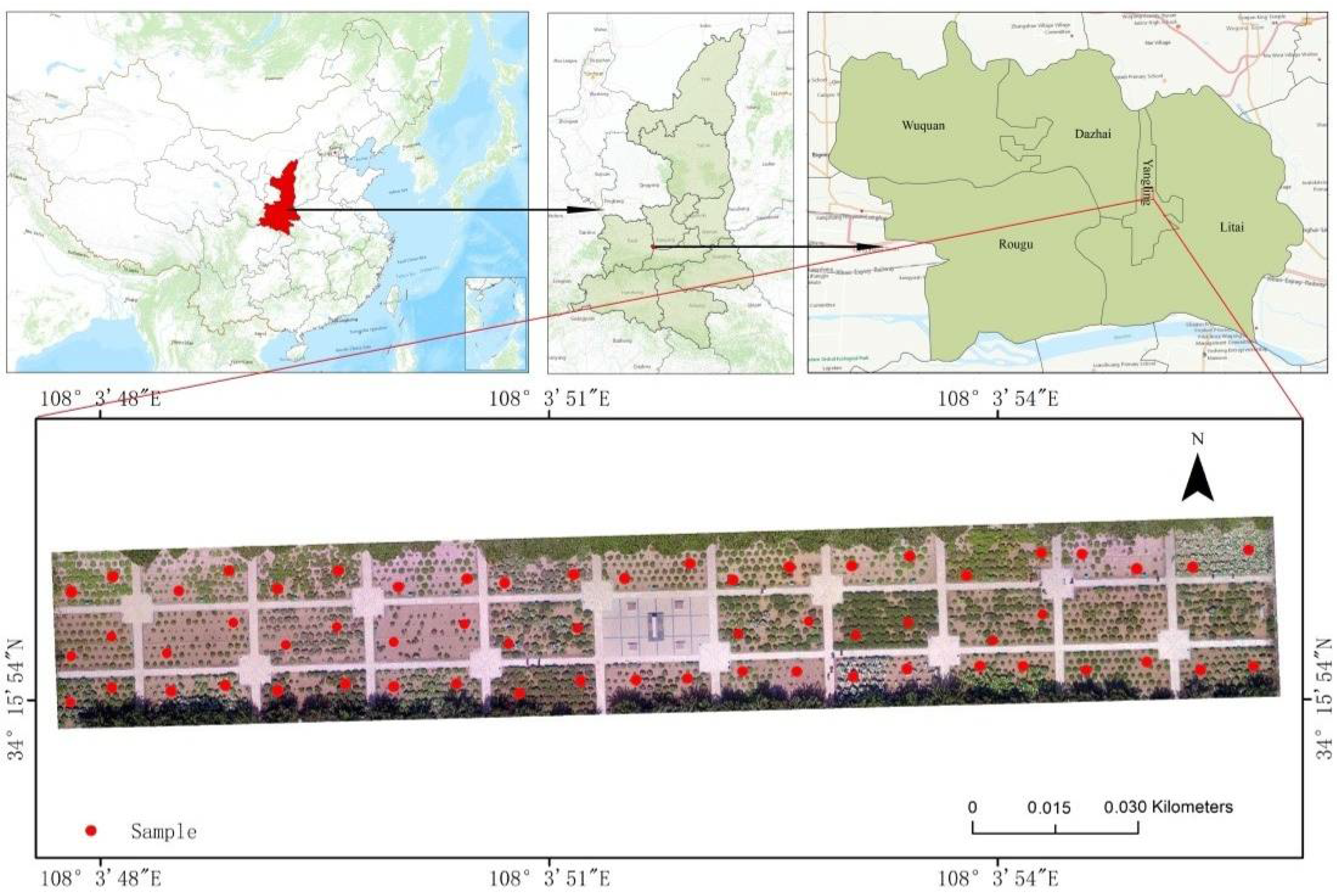
Figure 1. Location of study area and distribution of samples.
Remotesensing 14 02271 g001
Figure 2. Spectrometer and tree peony samples.
Remotesensing 14 02271 g002
Figure 3. Unmanned aerial vehicle (UAV) image mosaic and information extraction.
Remotesensing 14 02271 g003
Figure 4. Characteristics of original spectrum, first-order differential (FD) spectrum and continuum removal (CR) spectrum of tree peony leaves.
Remotesensing 14 02271 g004
Figure 5. Principal component analysis (PCA) results of tree peony leaves spectra.
Remotesensing 14 02271 g005
Figure 6. Coefficients of determination (R2) contour maps of ratio vegetation index (RVI), differential vegetation index (DVI), normalized vegetation index (NDVI) and soil-regulated vegetation index (SAVI).
Remotesensing 14 02271 g006
Figure 7. Distribution of measured Anth and predicted Anth in the random forest (RF) models: (a,b) are the calibration set and test set of the RF model based on principal component analysis using an unmanned aerial vehicle (PCA + UAV); (c,d) are the calibration set and test set of the RF model based on first-order differential using an unmanned aerial vehicle (FD + UAV); (e,f) are the calibration set and test set of the RF model based on continuum removal using an unmanned aerial vehicle (CR + UAV).
Remotesensing 14 02271 g007
Table 1. Statistical analysis of calibration-set Anth and test-set Anth.
TypeNMin (μg/cm2)Max (μg/cm2)Mean (μg/cm2)SDVarianceCV (%)
Calibration set400.0510.1710.1010.0280.00127.722
Test set200.0560.1690.1020.0270.00126.732
Note: Coefficient of variation (CV); standard deviation (SD); number (N).
Table 2. “Three-edge” parameters based on first-order differential (FD) spectrum.
ParametersDefinesFormulasReferences
λrWavelength corresponding to the maximum reflectivity in the 680–760 nm region of the FD spectral curveλDr[29]
DrMaximum reflectance of FD spectral curve in 680–760 nm regionMax(D680–760)[29]
SDrArea of FD spectral curve in 680–760 nm region 680 760 d R ( λ ) [29]
λyWavelength corresponding to the maximum reflectivity of the 560–640 nm region in the FD spectral curveλDy[30]
DyMaximum reflectance of FD spectral curve in 560–640 nm regionMax(D560–640)[30]
SDyArea of FD spectral curve in 560–640 nm region 560 640 d R ( λ ) [30]
λbWavelength corresponding to the maximum reflectivity of the 490–530 nm region in the FD spectral curveλDb[30]
DbMaximum reflectance of FD spectral curve in 490–530 nm regionMax(D490–530)[30]
SDbArea of FD spectral curve in 490–530 nm region 490 530 d R ( λ ) [30]
Note: first-order differential (FD).
Table 3. Absorption parameters of continuum removal (CR) spectrum.
ParametersDefinesFormulasReferences
TAIntegral of the depth of the band from the beginning to the end of a continuum λ m i n λ m a x d R ( λ ) [38]
LAIntegral area range from the wavelength corresponding to the maximum absorption depth to the left absorption peak λ m i n λ p e a k d R ( λ ) [38]
RAIntegral area range from the wavelength corresponding to the maximum absorption depth to the absorption peak on the right λ p e a k λ m a x d R ( λ ) [38]
SRatio of left area of absorption peak to right area of absorption peak L A R A [38]
NMADRatio of maximum absorption depth to total area of absorption peak 1 R ( λ p e a k ) T A [39]
ADmaxMaximum absorption depth 1 R ( λ p e a k ) [40]
PWavelength corresponding to the maximum absorption depth λ p e a k [38]
Note: R′ indicates the continuum-removed reflectance value.
Table 4. RGB (red–green–blue) vegetation index.
ParametersFormulasReferences
Visible atmospherically resistant index VARI = G R G + R B [42]
Red–green ratio index RGRI = R G [43]
Green–red vegetation index GRVI = G R G + R [44]
Normalized green–red difference index NGRDI = G 2 R 2 G 2 + R 2 [44]
Normalized green index NGI = G R + G + B [45]
Normalized blue index NBI = B R + G + B [45]
Normalized red index NRI = R R + G + B [45]
Dark green color index DGCI = H 60 180 + ( 1 S ) + ( 1 V ) 3 [46]
Note: R, G, and B represent the gray values of red, green, and blue bands respectively.
Table 5. Correlation between principal components, “three-edge” parameters, spectral absorption parameters and Anth of tree peony leaves.
Principal
Components
Pearson
Correlations
“Three-Edge”
Parameters
Pearson
Correlations
Absorption
Parameters
Pearson Correlations
400–550 nm550–788 nm400–788 nm
F10.28 *λr−0.50 **TA0.02−0.50 **−0.38 **
F20.28 *Dr0.31 *LA0.06−0.46 **−0.33 *
F3−0.15SDr0.19RA−0.13−0.54 **−0.54 **
F4−0.35 **λy−0.35 **S0.170.54 **0.47 **
F5−0.35 **Dy0.08NAD−0.030.63 **0.37 **
F6−0.15SDy0.13BDmax−0.01−0.10−0.12
F70.02λb−0.21P−0.48 **−0.010.15
F80.37 **Db0.31 *----
F90.01SDb0.39 **----
Note: F1F9 were the principal components extracted by PCA spectra; λr, Dr, SDr, λy, Dy, SDy, λb, Db and SDb are parameters based on position, amplitude and area of R, G, B bands; TA, LA, RA, S, NAD, BDmax and P are the absorption parameters extracted by the CR spectrum. ** p < 0.01, * p < 0.05.
Table 6. Correlation between RGB VIs, texture parameters, and Anth of tree peony leaves.
RGB VIsPearson CorrelationsTexture ParametersPearson Correlations
RGB
VARI−0.46 **Range0.230.28 *0.31 *
RGRI0.45 **Mean0.53 **0.29 *−0.02
GRVI−0.44 **Variance−0.25 *0.25 *−0.28 *
NGRDI−0.44 **Entropy0.220.190.23
NGI−0.11Skewness0.110.180.33 **
NBI−0.20----
NRI0.53 **----
DGCI−0.60 **----
Note: ** indicates p < 0.01, * indicates p < 0.05.
Table 7. Anth estimation models based on principal component analysis (PCA), first-order differential (FD), and continuum removal (CR) spectra.
Transform ProcessingModelsVariablesCalibration SetTest Set
R2cRMSEcREPc
(%)
R2vRMSEvREPv
(%)
PCAMSR80.450.0323.410.210.0431.72
PLS90.520.0221.810.440.02925.63
BPNN-0.690.0215.530.580.0439.27
RF70.910.0113.530.460.0327.07
FDMSR120.590.0220.050.560.0322.76
PLS110.530.0221.710.560.0222.31
BPNN-0.720.0218.050.590.0431.23
RF110.910.0110.450.510.0325.19
CRMSR130.630.0219.220.340.0328.32
PLS150.570.0220.620.340.0327.94
BPNN-0.590.0221.070.270.0329.47
RF120.870.0113.020.250.0329.85
Table 8. Anth estimation model based on unmanned aerial vehicle (UAV) parameters.
ModelsVariablesCalibration SetTest Set
R2cRMSEcREPc
(%)
R2vRMSEvREPv
(%)
UAV-MSR150.600.0219.870.270.0328.73
UAV-PLS180.490.0222.440.250.0328.77
UAV-BPNN-0.620.0220.050.290.0328.54
UAV-RF130.710.0219.170.450.0327.07
Table 9. Multisource remote sensing (RS) Anth estimation models.
Multisource SpectrumModelsVariablesCalibration SetTest Set
R2cRMSEcREPc
(%)
R2vRMSEvREPv
(%)
PCA + UAVMSR220.730.0216.350.340.0438.64
PLS210.750.0216.350.370.0441.47
BPNN-0.730.0216.530.580.0323.09
RF160.920.0112.640.560.0327.30
FD + UAVMSR230.830.0111.020.650.0221.48
PLS210.750.0116.560.710.0217.65
BPNN-0.850.0111.480.690.0219.43
RF170.930.018.250.760.0216.37
CR + UAVMSR240.870.0111.570.350.0328.99
PLS250.610.0331.580.370.0331.59
BPNN-0.730.0217.440.560.0324.48
RF150.910.0112.640.520.0326.91
Publisher’s Note: MDPI stays neutral with regard to jurisdictional claims in published maps and institutional affiliations.