Abstract
With the rapid development of wind power generation, many marine wind farms have been developed on the offshore intertidal sandbank (OIS) along the coastal regions of Jiangsu Province, China during the last decade. In order to quantitatively assess the stability of offshore wind turbines and their induced topographic changes on the OIS, a digital elevation model (DEM)-based analysis supported by satellite remote sensing is adopted in the present study. Taking the Liangsha OIS at the middle of Jiangsu coast, China as the research area, we first used an enhanced waterline method (EWM) to construct the 30 m resolution DEMs for the years 2014 and 2018 with the embedment of tidal creeks to effectively express the detailed characteristics of the micro-terrain. Then, a hypothetical sandbank surface discrimination method (HSSDM) was proposed. By comparing the height difference between the hypothetical and the real terrain surface during the operation period, the wind turbine-induced topographic change rate (TCR) was estimated from the DEM of 2018. The results show that 73.47% of the 49 wind turbines in the Liangsha OIS have an erosional/depositional balanced influence on the intertidal sand body, 8.16% show a weak depositional influence, and 18.36% lead to weak erosion. The average erosional depth, 58.6 cm, reached nearly 6% to 10% of the maximum possible erosion estimated by the hydrodynamic model. Furtherly, using two DEMs for the years 2014 and 2018, the topographic change depths at the location of wind turbines were calculated. By comparing the wind turbine-induced terrain change with the naturally erosional/depositional depths of the OIS, the average contribution rate caused by the wind turbines achieved 42.17%, which meant that the impact of wind turbines on terrain changes could not be ignored. This work shows the potential of utilizing satellite-based remote sensing to monitor topographic changes in the OIS and to assess the influence of morphological variations caused by wind turbines, which will be helpful for offshore wind farm planning and intertidal environment protection.
1. Introduction
With the rapid development of the global economy, a great number of fossil resources are consumed yearly, which has led to increasingly serious global warming and energy security problems [1,2,3]. In recent years, alternative sources of energy, especially clean and renewable energy, such as hydropower, solar power, and wind power, have drawn significant interest worldwide [4,5]. Among them, wind power technology developed very fast and has become one of the power-generating technologies with the greatest potential in large-scale and commercial development applications [6,7]. China has abundant wind power resources in the northeast, northwest, and northern regions of the mainland and in the coastal area. Along its 18,000 km long coastline, many offshore wind farms have been developed over the last decade. The development of offshore wind power has become an important strategic support for China’s energy structure transformation.
In China, rich offshore wind power resources are mainly distributed in a nearly 10 km wide stripe along the coastal regions with water depths of 5 to 50 m [4]. Therefore, most offshore wind power plants that have been built or are under construction are located in intertidal zones and shallow water areas. As these wind turbines are constructed on the offshore intertidal sandbank (OIS), they inevitably impact local tidal currents and waves, leading to erosion or deposition around the piles, and alteration of sandbank topography.
To determine the morphological changes that occur in the OIS and to quantitatively evaluate the erosional/depositional influences of wind turbines on sandbanks, hydrodynamic simulation is a commonly used method [8]. According to the hydrodynamic model simulation in the Huaneng Rudong intertidal wind power project located in the middle-eastern region of Jiangsu coast, the estimated erosional depth at the site of the wind turbine on the OIS is between 5.93 and 9.15 m, and the maximum radius of the scour pit is 12.64 to 17.90 m [9]. Hydrodynamic analyses can present extreme or final situations of sandbank erosion/deposition caused by wind turbines, but it is difficult to reveal the real spatial topographic change status during the wind farm operation period.
From the perspective of spatial analysis, the digital elevation model (DEM), a rectangular grid dataset interpolated by points of known elevation from sources, such as ground surveys or photogrammetric data capture to represent the relief of a terrain surface, provides an ideal solution for OIS terrain change detection [10,11]. Compared with different intertidal sandbank DEM data collection methods, such as ship-based echo sounding, airborne stereo-photogrammetry, and airborne light detection and ranging (LiDAR), satellite remote sensing provides a safe and cost-effective way for the topographic monitoring of the OIS located in places that are poorly accessible or potentially hazardous [12,13,14]. By interpolating a time series of waterlines with height information extracted from remote sensing images at different tidal periods, the conventional waterline method can quickly construct the DEM of the intertidal sandbank and show its surface undulations [15,16,17,18]. However, the resulting DEM has some shortcomings in explaining the terrain changes caused by small targets (e.g., wind turbines), both in the DEM construction and in the expression of terrain details.
Firstly, as a massive number of multi-temporal and multi-source satellite remote sensing image data are available, the waterlines precisely extracted from these images densely cover the whole intertidal flat surface. Some of the waterlines inevitably intersect others due to slight changes in the terrain or shift on the position of tidal creeks. They fragment the DEM and make it difficult to describe the overall terrain variation trend [18,19]. Secondly, the height differences on muddy coasts are relatively small. Several waterlines with similar heights easily cluster together, especially under low tidal conditions. A suitable method is needed to determine a characteristic line to represent the spatial location and elevation information contained in these small tidal-height intervals [20]. Thirdly, the DEMs constructed by the conventional waterline method usually has a relatively coarse spatial resolution. It cannot effectively express the morphological changes caused by tidal creeks of various widths and shapes on the surface of sandbanks. However, these kinds of micro-topographical characteristics are important to reveal the terrain change impacts of small targets, such as wind turbines, exerting on the sandbanks. Finally, a DEM interpolated by shorelines with height characters cannot take into account the presence of wind turbines during its construction process. Therefore, using the DEM to determine the terrain differences caused by wind turbines and analyzing the inter-influence between the variation in sandbanks and wind turbines is a great challenge.
The main objective of this paper is to provide a feasible way to evaluate topographic changes caused by the construction of offshore wind turbines on their located OIS based on the support of satellite remote sensing and DEM spatial analysis techniques. The innovation points are: (1) modify the conventional waterline method to allow the constructed DEM to better describe the detailed terrain character in the quick and easily changed OIS, (2) propose a novel method to quantitatively estimate the topographic changes caused by the construction of wind turbines from the remote sensing constructed DEM, and (3) understand the contribution rate and manner for wind turbine-induced terrain changes to the natural topographic variations at the offshore sedimentary environments.
The remainder of the paper is structured as follows. In Section 2, we present the natural conditions of the study area. Section 3 describes the data used in this paper. In Section 4, we introduce the methodologies adopted in this paper, including OIS DEM construction, wind turbine-induced OIS topographic change estimation, and OIS topographic change intensity judgement. Section 5 shows the corresponding results and analysis obtained. Section 6 and Section 7 are our discussions and conclusions.
2. Study Area
Jiangsu Province is located on the middle-eastern coast of China. Along its open coast facing the southern Yellow Sea, a unique radial sandy ridge system with more than 70 sand ridges and tidal channels extending approximately 200 km from north to south and 90 km from east to west has developed [21,22]. In the last decade, wind power has made rapid progress in the core region of the radial sandy ridge outside of JiangGang town. In this study, the Liangsha area (Figure 1), especially the Jiangjiasha and Zhugensha sand bodies, was selected as a test site for the DEM generation and wind turbine-influenced morphological change analysis.
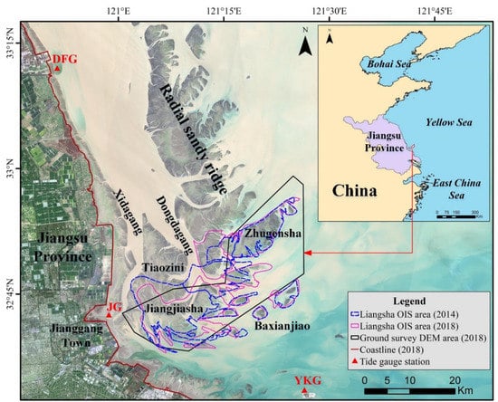
Figure 1.
Location map of the Liangsha offshore intertidal sandbanks with the distribution of three tidal gauge stations. The background image is a Sentinel-2 false-color image acquired on 9 April 2018.
The Liangsha area is macro-tidal with a semi-diurnal tidal range of 3.9 m to 5.5 m [21]. Due to wave energy attenuation on shallow water sandbanks, the wave action is extremely weak. Maximum currents over the intertidal sandbank range from 0.5 to 1.0 m/s [23]. Over the last decade, the Liangsha OIS has shown obvious and continuous topographical variations under the effects of natural and anthropogenic processes [12,18,19,24,25]. With the coastal land reclamation of the Tiaozini sandbank on the west side, two large tidal channels in the north part of the Liangsha sandbank, namely the Dongdagang channel and Xidagang channel, were forced to swing and broaden towards the seaside. They control the shape, position, and movement of the Liangsha OIS. On the OIS surface, many dendritic tidal channels are observed on the Jiangjiasha sand body and through-type tidal channels on the Zhugensha sand body. These channels affect the undulations of the sandbank surfaces and lead to micro-topographic variations in these areas.
3. Materials and Data
In this study, a DEM-based analysis with the support of remote sensing was adopted to assess the morphological changes of the OIS induced by the construction of wind turbines. Four datasets were collected, and the processing details are described below.
3.1. Satellite Image Data
Near the Liangsha OIS, the Jiangjiasha 300-MW and the Huaneng Rudong 300-MW offshore wind farms were developed in 2017 and 2016, respectively (Figure 2). To compare the topographic changes that occurred in the sandbanks during the construction processes of these two wind farms, satellite remotely sensed image data covering the years 2014 and 2018 were collected. For 2014, 21 scenes of 16 m spatial resolution images acquired by the Chinese-launched GF-1 satellite were selected. Additionally, for 2018, a total of 80 scenes of Landsat 8 OLI satellite image data and Sentinel-2 satellite image data with spatial resolutions of 30 m and 10 m were used. All these collected images were first atmospherically corrected using the Envi5.3 FLAASH atmospheric correction tools [26]. Then, they were geometrically registered to the WGS84 coordinate system and the Universal Transverse Mercator North 51st zone projection system. Finally, all the collected images with different spatial resolutions were re-sampled to 30 m to match the maximum diameter of the scour pits around the wind turbine piles.
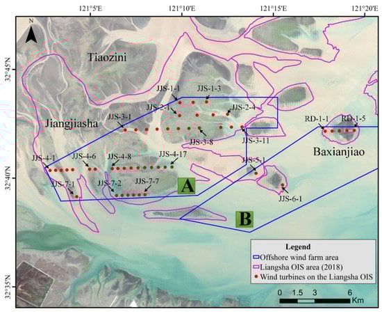
Figure 2.
Spatial distribution of 49 offshore wind turbines in the Liangsha OIS. The irregular polygons labeled A and B are the regions of the Jiangjiasha 300-MW and Huaneng Rudong 300-MW offshore wind farms, respectively.
3.2. Tidal-Height Data
Waterlines extracted from the re-sampled remote sensing images had no associated height information. Data representing the tidal heights at the image acquisition times would be helpful in assigning heights to them [16]. In the present study, we used a classical tidal harmonic analysis, which was a kind of location-based estimation method for tidal-height simulations [27]. From north to south, three tidal gauge stations, namely, Dafenggang (DFG), Jianggang (JG), and Yangkougang (YKG), surrounding the Liangsha OIS area were selected. Their locations are shown in Figure 1. Hourly tidal-height data collected at these stations for the year 2018 were acquired. Then, T_TIDE, a MATLAB-version tidal harmonic analysis software package, was applied to obtain the harmonic parameters for each gauge station [28]. Eight fundamental tidal constituents, K1, O1, M2, S2, N2, K2, M4, and MS4, were selected to represent the effects of tidal forcing in the Liangsha area [29,30]. As the tidal harmonic constituents, station latitudes, and satellite overpassing times were input into the T_TIDE package, the tidal height at each image acquisition time, together with the error estimation, was obtained. After validation by the actual tidal heights measured at the DFG tidal gauge station during 17–19 July 2018, the root-mean-square error (RMSE) was found to be less than 20 cm, with a correlation coefficient reaching 0.98.
3.3. DEM Validation Data
At the end of the year 2018, during the period of high water level, an underwater topographic survey covering the Liangsha sandbank (Figure 1) was carried out by using a combination of ship-based echo sounding and GPS-RTK (global positioning system-real-time kinematic) positioning. The spacing between the elevation points observed on site was 100 to 300 m. An interpolated DEM with a spatial resolution of 250 m was generated by the Ordinary Kriging interpolation method and used to validate the accuracy of the resulting intertidal DEM generated by remotely sensed waterlines.
3.4. Wind Turbine Data
The analysis of Sentinel-2 high-spatial-resolution satellite remote sensing images for the years 2016 to 2018 revealed many offshore wind turbines within the offshore sandbanks. Taking the common scope of the Liangsha OIS area in 2014 and 2018 as a reference, the locations of 49 wind turbines on the Liangsha OIS were automatically extracted from the geo-rectified Sentinel-2 satellite data imaged on 9 April 2018. Figure 2 shows their spatial distribution. These wind turbines were arranged in eight rows, of which seven rows were located in the Jiangjiasha sea area and labeled from JJS-1 to JJS-7, and one row was located in the Baxianjiao sea area with the label of RD-1.
4. Methodology
The assessment of marine wind turbine-induced topographical changes in the OIS involves two main methods: (1) the enhanced waterline method (EWM), to construct the high-accuracy DEM, which can meet the need to monitor variations of small targets spatially, and (2) the hypothetical sandbank surface discrimination method (HSSDM), to analyze the topographical changes caused by the wind turbines based on the DEM dataset. The overall methodology of the study is shown as a flowchart (Figure 3).
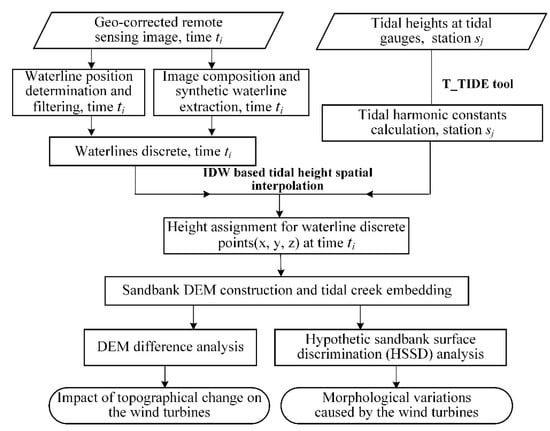
Figure 3.
Flow diagram of the proposed methodology adopted in the study.
4.1. OIS DEM Construction
Compared with the wide and flat OIS spreading for several square kilometers, the slender wind turbines with small bases erected on sandbanks can be regarded as tiny targets. In order to reveal the topographic changes caused by these kinds of tiny targets, a more accurate DEM with better-detailed terrain characters is needed. The EWM is proposed here for OIS DEM construction and the improvements of the method are presented in these main ways:
- (1)
- Dense waterline filtering and height assignment
An offshore intertidal sandbank is commonly characterized as broad and gentle, with many shallow tidal channels radially distributed to show the rhythmic undulation of the flat surface. Even though the height differences among the studied sandbanks were usually small, the waterlines also obeyed the overall variation trend of diminishing elevation from the top of each sandy ridge to its low tidal edge. After the waterlines from 80 remote sensing scenes in the year 2018 were extracted, they were first roughly filtered by their shapes and locations. Those waterlines with obviously chaotic locations or intersecting with other regularly distributed ones were removed to keep the rest spatially separable. Then, the consistency of the tidal-height relations of the remaining waterlines was checked to ensure the rationality of their indicated terrain variation trends. Since each reserved waterline had three estimated tidal heights calculated from the DFG, JG, and YKG stations by T_TIDE tools, they were sorted by their tidal heights, and a linear fitting analysis was performed. By comparison, we chose tidal heights with a relatively good linear fit at all three tidal gauge stations as the candidate scenario. The tidal heights with the best linear fitting effects among the three stations were temporarily assigned to their corresponding waterlines. Judging by the tidal level relation, if the height relationship between a given waterline and either of its neighbors was wrong or did not match the gentle variation trends of the terrain, it would also be removed. Finally, qualified waterlines from 37 scenes were kept.
- (2)
- Image composition and synthetic waterline extraction
After sorting the 37 retained waterlines by their tidal heights, it was found that four, three, five, five, and seven waterlines were spatially crowded in five narrow plane strips, and were all clustered in small tidal-height intervals ranging from 13 cm to 40 cm. The remaining 13 waterlines were spatially distributed among the wide intertidal flat. Aside from introducing interpolation errors and leading to the fragmentation of the resulting DEM, such a number of waterlines gathered together is not beneficial for the construction of the DEM. Hence, an improved image compositing approach [20] was applied to obtain the representative synthetic waterline from the generated composite image to solve this problem. For the five selected remote sensing image datasets corresponding to the grouped waterlines, the modified normalized difference water index (MNDWI) was adopted for the image composition owing to its ability to effectively enhance the characteristics of open water and suppress the soil noise in exposed offshore sand bodies [30,31]. Considering that there were less than 7 images participating in the layer stacking process and no extreme values existed, the average-value calculation of the MNDWI was more suitable than the median-based calculation. Therefore, combined with the average value of the MNDWI for each pixel, five stacked images were respectively generated. By detecting the land–sea edges from the threshold-segmented MNDWI compositing images using a Sobel operator [30], the corresponding synthetic waterlines were produced. They could effectively represent the average locations and height characteristics of these clustered waterlines.
- (3)
- Tidal channel embedment
All the waterlines, including directly extracted and synthetic, were then separated into discrete points with an interval of 30 m. After assigning tidal-height values to these discrete points, the initial DEM for the studied OIS could be interpolated using an inverse distance weighting method [12,30]. However, the interpolation process for the generation of DEM smoothed the tiny undulations of the intertidal flat surface, especially within the height difference of 30 to 50 cm, which was equivalent to the depth of the small tidal channel winding on the sandbank. Therefore, tidal channels with varied shapes and widths on the sandbank surface are ideal candidates with which to express the rhythmic oscillation characteristics of the terrain.
From the Sentinel-2 satellite remote sensing image acquired during the mean spring low-tidal level, we precisely delineated the plane boundary lines of the tidal channels on the OIS and simultaneously extracted their middle lines. The boundary lines were adopted to control the spatial locations and the width variations of the tidal channels. Additionally, the middle lines were used to help construct the inner terrain of the tidal channels. Since the middle lines only had associated location information and no elevation information, the lowest tidal heights estimated at the three tidal gauge stations during the year 2018 were treated as the base height values. Additionally, for the boundary lines, the tidal heights at the image acquisition time could be directly used. Then, the height information was assigned to the spatially discrete points of the middle lines and the boundary lines by the inverse distance weighted (IDW) interpolating method, and a tidal channel DEM showing the basic flow network structures was generated. By embedding the tidal channel DEM into the initially constructed DEM, the final OIS DEM with detailed tidal surface terrain fluctuations could be obtained.
Another way to obtain the final OIS DEM was to put all elevation discrete points representing tidal channels and waterlines together for DEM construction. However, after comparing the resulting DEM obtained by this processing method with the tidal channel embedding method, it was observed that the latter result performed more naturally in its illustration of micro-terrain fluctuation variations. Therefore, the OIS DEM constructed by the tidal channel embedding method was adopted for the subsequent terrain change analysis.
4.2. Wind Turbine-Induced OIS Topographic Change Estimation
A hypothetical sandbank surface discrimination method (HSSDM) was proposed to detect the wind turbine-induced topographic change and its contribution to terrain variation from DEM constructed by remote sensing. Using the HSSDM to calculate the wind turbine-induced OIS topographic change, two surfaces of different elevations are needed. The surface from the OIS DEM at the central location of the wind turbine (red line in Figure 4a) can be treated as the real terrain surface. However, another surface is missing. Here, we assume that a hypothetical sandbank surface (black, dashed line in Figure 4a) exists to represent the virtual sandbank situation at which there is no wind turbine constructed. Then, by calculating the height difference, ΔH, between these two surfaces, we can evaluate the erosional/depositional variations caused by the construction of the wind turbine. The formula for the topographic change height (∆H) calculation is as follows:
where is the elevation of the real sandbank surface, which can be directly extracted from the DEM, and is the hypothetical sandbank surface elevation (HSSE).
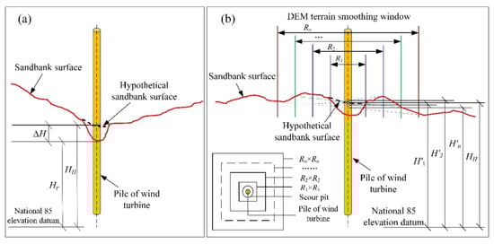
Figure 4.
The schematic diagram for the HSSDM. (a) Topographic change height (ΔH) calculation for the area around the wind turbine. (b) Estimation of HH from the average heights of a series of smoothing windows of different sizes.
Figure 4b shows the HSSE estimation method by the smooth-window averaging process. Taking the central location of a given wind turbine as the center of the terrain smoothing window, we can set a series of windows with different sizes, Ri. These windows cover different areas of the sandbank surface that may contain tidal ridges, tidal channels, or both, and have varied mean elevations. Naming the mean elevation of the window i as the variable, it shows the undulation of the background terrain under different sizes around the wind turbine. Therefore, if the sizes and number of the windows are determined, the average value of can be treated as the HSSE to represent the mean variation of the background terrain as there is no wind turbine built.
In the Liangsha OIS area, considering that the spatial resolution of the DEM was 30 m and the minimum distance between two adjacent wind turbines was less than 480 m, 10 groups of windows were preliminarily set to have sizes of 45 m, 60 m, 75 m, 90 m, 105 m, 120 m, 150 m, 240 m, 300 m, and 480 m. By resampling the spatial resolution of the DEM to these pre-defined window sizes, we could obtain a series of mean elevations, (i = 1,2,…, 10), for all the wind turbines in the wind farm under these specified smoothing window areas. These mean elevations for each wind turbine were then plotted orderly in a line graph to illustrate their terrain variation trends with increasing window sizes. It was found that the showed small oscillations, especially when the window size was less than 120 m, reflecting the tiny topographic undulations of the studied OIS around the wind turbines.
Furthermore, a cross-correlation analysis for these average terrain heights of 10 groups of window sizes was carried out and the resulting line charts of the cross-correlation coefficients for the HSSE are shown in Figure 5. It was found that with the increase in the window size, the cross-correlation relationship of the HSSE decreased in a power function trend. Two extreme minimal cross-correlation coefficient values appeared at window sizes of 120 m and 300 m. However, the larger the window size, the smoother the effect on the hypothetical sandbank surface terrain. The bigger window size was not conducive to the expression of micro-morphological change. Therefore, the size of 120 m was confirmed to be the maximum smoothing window size. It could also be regarded as the probable maximum diameter that the wind turbine had an influence on the terrain.
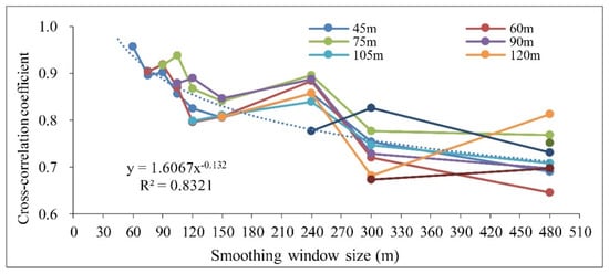
Figure 5.
The variation trends of the cross-correlation coefficient for the HSSE calculated under the specified smoothing window sizes of 45 m, 60 m, 75 m, 90 m, 105 m, 120 m, 150 m, 240 m, and 300 m.
Then, the HSSE averaged by the mean elevations of the sandbank under the sizes of 45 m, 60 m, 75 m, 90 m, 105 m, and 120 m, representing the hypothetical sandbank surface at the central location of each wind turbine, was calculated as follows:
where is the HSSE at the central location of the wind turbine, is the mean elevation under different sizes of windows obtained from their corresponding resampled DEMs, and is the number of smoothing windows.
4.3. OIS Topographic Change Intensity (TCI) Judgement
As the height difference, ΔH, caused by the construction of wind turbines was obtained, we used the annual erosion/deposition depth, also named the topographic change rate (TCR), to determine the wind turbine-induced topographic change intensity (TCI) of the OIS. It is calculated as follows:
where is the time period from the beginning of the wind farm construction to the date that the constructed DEM represents.
For the TCI judgement criteria, three sets of analysis data relevant to the Liangsha OIS area were referenced here. The first is the mean error of the DEM constructed by the conventional waterline method and the value is approximately 45 cm at the fan-shaped radial sand ridges of the Jiangsu offshore area [18]. The second is the standard deviation of the constructed DEM, which is approximately 80 cm. Additionally, the third is the range of the elevation variation of the Liangsha OIS area, which is approximately 400 cm. Here, we finally selected 40 cm, which is approximately 1, ½, and 1/10 times the value of the three above-mentioned reference datasets, as the annual topographic change interval to define the degree of erosional/depositional height. Then, the judgement criteria for the TCI grade in the OIS areas are listed in Table 1. The degree of morphological change for the offshore sandbanks is divided into five grades: heavily erosional, weakly erosional, balanced, weakly depositional, and heavily depositional. Depending on the variation range of the TCR, we can judge the TCI and assess the influence caused by the construction of wind turbines on the sandbanks.

Table 1.
Judgement criteria for the different grades of TCI in the Liangsha OIS.
5. Results
5.1. DEM of Liangsha OIS Area
Using the EWM, two DEMs of the Liangsha OIS area representing 2014 and 2018 were constructed at a spatial resolution of 30 m (Figure 6). An upscaling conversion was performed to resample the remote sensing constructed DEM to 250 m to match the resolution of the ground-measured DEM data. Then, the overlapping part of these two DEMs was clipped for the accuracy assessment.
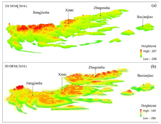
Figure 6.
The 3D format of Liangsha OIS DEM constructed by the EWM. (a,b) are the DEMs for 2014 and 2018, respectively.
By comparison, the elevation ranges for the constructed DEMs were between 2.07 m~−2.96 m in 2014 (Figure 7a) and 1.49 m~−2.86 m in 2018 (Figure 7b). These values were similar, but smaller than the measured DEM of 1.82 m~−5.26 m. The difference in elevation range is attributed to the time duration that each DEM represented. The measured DEM was good at showing the actual state of the terrain over a short measurement period. Therefore, it showed a relatively large elevation range. However, the DEMs constructed by remote sensing were derived from nearly a year of waterline time series. Over this longer time interval, the terrain was smoothed by the averaging effect of its dynamic changing. Therefore, the simulated vertical variation of the terrain was smaller.
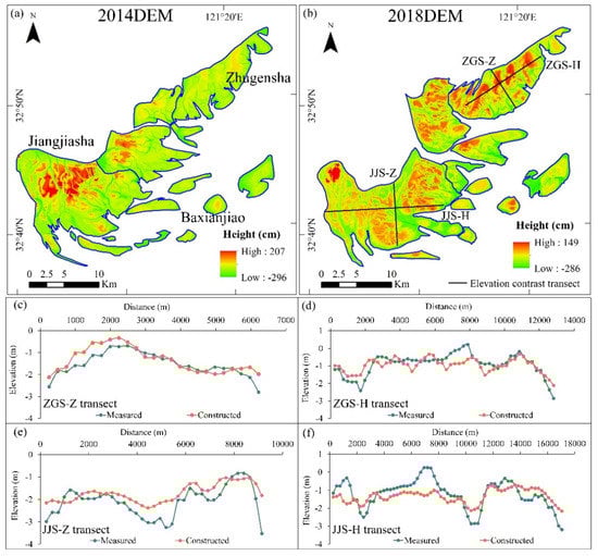
Figure 7.
DEM accuracy analysis. (a,b) are the plain view of Liangsha OIS DEM. (c–f) compare measured and constructed DEM elevations along transects ZGS-Z, ZGS-H, JJS-Z, and JJS-H for the year 2018.
Within the Liangsha OIS area, we set four contrast transects. Their locations are shown in Figure 7b. Four transects all showed good linear correlations between the measured and inversed elevations (Figure 7c–f). The linear correlation coefficients were 0.85, 0.76, 0.75, and 0.65, respectively, and all met the significance level of p-value less than 0.005. The mean absolute error of inversed elevations at these transects varied from 27 cm to 51 cm, with an average value of 40 cm. By comparing the morphologies of these four transects, it can be observed that the locations of large tidal channels had a good consistency, except that the surface of the sandbank shown in the constructed DEM was relatively gentle and the degree of undulation was smaller than that in the measured DEM.
5.2. Topographical Changes Caused by the Wind Turbines
By calculating the elevation difference at the central locations of the 49 OIS wind turbines between the remote sensing constructed DEM surface and the hypothetical sandbank surface standing for the average height of the background terrain during the operation of the wind farms, we obtained the OIS TCRs together with their TCI grades at the location of wind turbines (Figure 8).
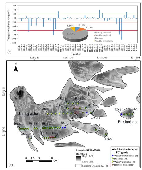
Figure 8.
Topographic change caused by the construction of wind turbines. (a) TCR of the 49 wind turbines. Red lines show the threshold for different TCR intervals defined in Table 1. Additionally, the pie chart illustrates the ratio of the wind turbines in different TCI grades. (b) Spatial distribution of their TCI grades.
According to the TCR judgement criteria, 4 out of the 49 wind turbines in the Liangsha OIS area caused heavy erosion of the sandbank, occupying 8.16% of the total number of wind turbines. The maximum TCR reached −103.35 cm/a. Five wind turbines led to weak erosion of the sandbank with an average TCR of −39.27 cm/a, accounting for 10.21%. Erosional/depositional balanced states were found in 36 turbine locations and showed the largest proportion of 73.47%. The average TCR at these points was −1.08 cm/a, which showed that the effect these wind turbines exerted on the sandbank was biased towards slight erosion. Additionally, the remaining four wind turbines were weakly depositional, which occupied 8.16%. The maximum TCR was 39.9 cm/a.
Based on the proportion of the TCI, nearly 3/4 of the wind turbines were categorized as having an erosional/depositional balanced topographic change status. Only 18.36% showed a certain degree of erosion, and the average erosion depth of 58.6 cm was much smaller than the maximum possible scour pit erosion depth of 6–9 m estimated by the hydrodynamic model simulation [9]. Therefore, under the present situation, the development of wind farms in the Liangsha OIS area had a small impact on the morphology of the intertidal sandbank.
Observed from the spatial distribution of TCI grades (Figure 8b), four wind turbines that caused heavy erosion of the sand body were located in the deep and narrow tidal channels. These tidal channels, which originated from the sand ridge and oriented towards the sea, were directly born and developed by the construction of wind turbines. As tidal flows passed through each wind turbine pile, the boundary layer was separated and the streamlines were concentrated. This change in the local flow pattern increased the bottom shear stress and improved the sediment carrying capacity of the flow. Then, the surface of the sandbank could easily rush into narrow and deep tidal channels, causing heavy erosion around the wind turbines. The 36 wind turbines that led to erosional/depositional-balanced sandbank statuses were mainly distributed in the higher surfaces of the intertidal area. The topography of these locations was relatively smooth and had small height differences from the surrounding areas. Therefore, the influences of the piles blocking the surface flow and reducing sediment transport were slight. Four wind turbines that caused weak deposition of the sandbank were located at the edge of the higher sand ridge surface area adjacent to large tidal channels, and the surrounding beach surface was lower. In this situation, the existence of wind turbines would promote minor siltation of the sandbank surface.
5.3. Influence of Topographic Change on the Safety of Wind Turbines
Based on two DEMs in the years 2014 and 2018 representing the morphology before and after the construction of the Liangsha wind farm, elevation variations were calculated to analyze the impact of topographic changes on the safety and stability of the wind turbines. The erosional/depositional depths at the central positions of the 49 OIS wind turbines were divided into three groups, which are shown in Figure 9. The locations of seven wind turbines were weakly erosional with erosion depths ranging from −198 cm to −80 cm, and 11 locations were weakly depositional with deposition depths between 80 cm and 106 cm. They, respectively, occupied 14.29% and 22.45% of the total number of wind turbines in the Liangsha OIS. The locations of the remaining 31 wind turbines were in the erosional/depositional balanced state, accounting for 63.27%.
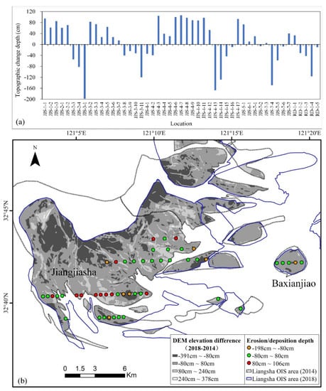
Figure 9.
Topographic changes of the Liangsha OIS between 2014 and 2018. (a) Topographic change depths of the Liangsha OIS at the locations of the 49 wind turbines. (b) Spatial distribution of three erosional/depositional depth groups.
From the perspective of spatial distribution characteristics, the locations categorized as weakly erosional were scattered either at the edge of the intertidal zone or in the small tidal channel of the sand body. Because of the reciprocating erosional action by tidal currents, some tidal channels became broader, and the edges of sandbanks collapsed gradually into the sea. Fine sediments were then washed out, suspended, and transported to the adjacent beach for siltation. Thus, there was a decrease in elevation at the locations of the seven weakly erosional points, with the average TCR reaching −34.32 cm/a and the maximum TCR reaching −49.56 cm/a during the four years. The 11 locations that were classified as weakly depositional were mainly distributed in the southern part of the Jiangjiasha sandbank. These positions were always on the ridge area of the sand body and were less affected by the swing of surface tidal channels. Suspended fine muds and silts on the north and west sides of the Jiangjiasha sandbank were carried south-eastward by tide-induced residual currents and were then deposited to form a relatively small siltation area. At these locations, the average TCR was 23.60 cm/a, and the maximum TCR reached 26.62 cm/a. The 31 erosional/depositional-balanced locations were widely distributed in the higher elevation area of the sandbank. The sandbank surface was overall in a minor siltation condition with a TCR of 2.28 cm/a.
Therefore, it could be concluded that the topography of the Liangsha intertidal sandbank where these wind turbines were erected was mainly in an erosional/depositional balanced to a weak siltation state. Under the current development intensities that included activities, such as intertidal flat reclamation, shellfish farming, and wind energy utilization, the topographic changes were still in a lower intensity range. The topographic changes occurring in the Liangsha OIS had a minor effect on the safety and stability of the local wind turbines.
5.4. Contribution of the Wind Turbines to Topographic Change
Assuming that the terrain changes were continuous, we took the 1/4 of the DEM elevation difference between the years 2014 and 2018 as the annual variation, and compared them with the wind turbine-induced topographic change depths at the central locations of the 49 wind turbines during the operation period of the wind turbines. Then, the contribution rates of terrain changes that wind turbines exerted on the Liangsha OIS were calculated and the results are shown in Figure 10.
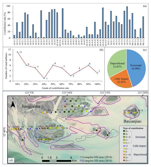
Figure 10.
Contribution of terrain changes caused by the construction of wind turbines. (a) Contribution rates of the 49 OIS wind turbines. (b) The number of wind turbines by their grades of contribution rates. (c) Terrain change types and their proportions that the wind turbines exerted on the OIS. (d) Types of contribution for terrain change at the locations of 49 wind turbines.
Among the 49 OIS wind turbines, 29 had a contribution rate smaller than 50%, which occupied 59.18%, and 20 greater than 50%, accounting for 40.82% (Figure 10b). The average contribution rate reached 42.17%, which meant that the contribution of wind turbines to terrain changes could not be ignored. Furtherly, according to the degree of contribution (Figure 10c), 11 wind turbines with a contribution rate of less than 10% were regarded to have little impact on the terrain change, occupying 22.45%. A total of 16 wind turbines caused the depositional effect and 22 wind turbines caused the erosional effect on the terrain changes, accounting for 32.65% and 44.90% of the total number of wind turbines, respectively.
Since the terrain changes caused by wind turbines and by natural forces may not synchronous, according to different terrain change types and their correspondent ranges of contribution rates, the detailed contributions that wind turbines exerted on the Liangsha OIS are categorized and listed in Table 2. For the type of contribution, ‘D’, ‘E’, and ‘LI’ represent depositional, erosional, and little impact, respectively. ‘-’ represents a slight decrease, ‘--’ represents a great decrease, ‘->’ means conversion, ‘+’ represents a slight increase, and ‘++’ represents a great increase. Figure 10d shows the types of contribution for terrain change at the locations of 49 wind turbines.
Table 2.
Different types of contributions that wind turbines exerted on the terrain changes.
For the 22 locations at which wind turbines caused terrain erosion, 45.15% of them (corresponding to D-- and D-) led to a reduction in natural deposition, which was mainly distributed at the ridges of sand bodies. Additionally, 31.82% of them (corresponding to D->E) located at narrow tidal creeks converted their natural terrain change status from deposition to erosion. The rest 22.73% (corresponding to E+ and E++) were mainly located at the broad tidal channels or at the edges of sand bodies, which resulted in the promotion of natural erosion.
Among the 16 locations at which wind turbines caused terrain deposition, 37.50% of them (corresponding to E-- and E-) were observed mainly positioned at the broad tidal channels or at the edge of the sand body, resulting in a decrease in natural erosion. Since broad channels were beneficial to the flow of tidal currents, the types of contributions at these locations were correspondent to the state of the terrain erosion under different levels. Additionally, 18.75% of them (corresponding to E->D) caused a change in the topographical status from erosion to deposition. Additionally, the other 43.75% (corresponding to D+ and D++) were positioned at the ridges of sand bodies, which led to an increase in the natural deposition.
6. Discussion
6.1. The Number of Windows for the Calculation of the Average HSSE
For the HSSDM, the key for the evaluation of terrain variation caused by the construction of wind turbines was the accurate estimation of the HSSE. The hypothetical sandbank surface used elevation information from the terrain surrounding the wind turbines. A total of 120 m was determined as the maximum size of the smoothing window, and the scheme of averaged heights for 45 m to 120 m with an increasing interval of 15 m was adopted for the estimation of the HSSE. In order to demonstrate the rationality of this simulation scheme, two scenarios, including 11 combinations of HSSE results, were evaluated (Figure 11).
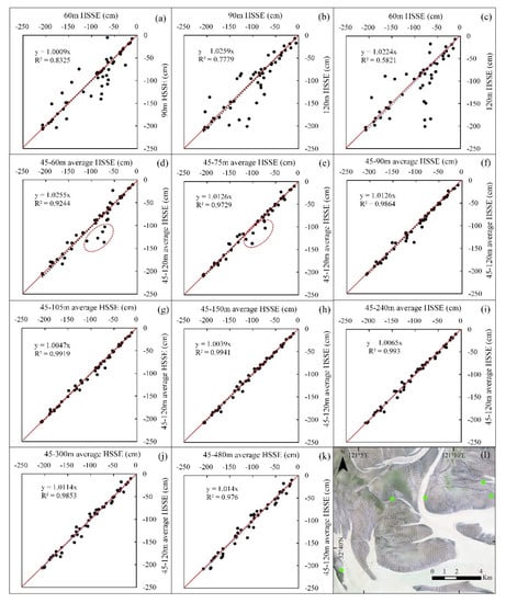
Figure 11.
Correlation analysis for HSSE results under different scenarios. (a–c) are the comparison under the single smoothing window. (d–k) are the comparison between the different average schemes and our adopted average scheme. (l) displays the actual locations of the five scattered points in (d,e).
The first scenario was to analyze the HSSE results calculated by the single smoothing window. The window sizes of 60 m, 90 m, and 120 m were chosen for the HSSE calculation and correlation analysis. Their linear correlations are shown in Figure 11a–c, respectively. As the window sizes and window size differences became larger, the linear correlation coefficient for the three combinations decreased from 0.91 to 0.76 and RMSE increased from 23.60 cm to 38.83 cm, respectively. The good linear correlation and low RMSE indicated that most areas in which wind turbines were erected were relatively smooth, thus using different window sizes for calculating the HSSE at these locations may have little difference. However, in those areas with larger undulations, e.g., sand ridge areas with densely distributed tidal channels, a single window was not appropriate for describing the variation of background topography. The smaller the window size, the greater fluctuations of the HSSE. Therefore, the average elevation for a series of different window sizes to obtain the HSSE is a good solution to describe the real terrain characteristics.
In the second scenario, we compared eight combinations of HSSE results between the average schemes of the different number of windows and our adopted average scheme. The linear fitting curve maps are shown in Figure 11d–k. As displayed in these figures, when a small number of windows participated in the calculation, the estimated HSSE results would be more scattered. The actual positions of five dispersed data points in the red ellipses of Figure 11d,e are mapped in Figure 11l. They were observed to be located at the edge of the sand body or directly in the tidal channel. Since the small-sized window covered areas with great terrain changes, it would lead to the dispersed HSSE value showing this kind of data oscillation. As the number of windows increased to the size of 120 m, the fluctuation of simulated HSSE would be reduced. However, when window sizes larger than 240 m participated in the elevation average process, the HSSE fluctuation would begin to increase again, as shown in Figure 11j,k. Therefore, the average scheme for the window size from 45 m to a maximum of 120 m was enough to represent the background terrain variation in the undulated intertidal sandbank area.
6.2. The Representativeness of the HSSE to the Actual Height of the Terrain
The DEM for 2014, where there were no wind turbines on the Liangsha OIS, was chosen to evaluate the representative effect for the estimated HSSE to the actual DEM height. To ensure the comparability of the results, we chose the same locations of the 49 wind turbines and extracted the terrain height directly from the DEM. The HSSE at these locations was calculated in the same way by our adopted average scheme.
The comparison between the HSSE and the DEM terrain height at the 49 locations together with the frequency histogram of their height differences are shown in Figure 12a,b. They had a good agreement and the linear correlation coefficient reached 0.97. The mean absolute error (MAE) was 7.21 cm and the standard deviation (SD) was 16.48 cm. Totally, 65.31% of the height difference between the DEM terrain height and the estimated HSSE were located within −5 cm to 5 cm and 87.76% within −10 cm to 10 cm (Figure 12b). Two points with higher height estimation error are circled in Figure 12a. Observed from the constructed DEM, JJS-3-2 was on the southern part of the Jiangjiasha OIS and rightly in a winding tidal trench with a width of about 120 m. JJS-4-4 was located at the southwest boundary of the OIS near the edge of a big tidal channel. In such a small area of rapidly changing topography, the calculated HSSE will have a relatively large error. However, on the whole, the HSSE calculated by the average of a series of rectangular smoothing windows with different sizes showed a good capability to represent the actual height of the terrain.
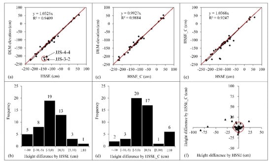
Figure 12.
The comparison of the HSSE with the DEM height of the terrain. (a) The linear correlation between the DEM elevation and the HSSE. (b) The frequency histogram showing the range of height difference by HSSE. (c,d) are the results between the DEM elevation and the HSSE_C. (e,f) are the linear correlation and the spatial distribution of height difference between the HSSE and HSSE_C.
Furthermore, we calculated the HSSE using a circular smoothing area with different diameters, named HSSE_C, to test the accuracy and convenience of the average smoothing method in the determination of terrain height. Taking the location of the wind turbine as the center of the circle, six circles with diameters of 45 m, 60 m, 75 m, 90 m, 105 m, and 120 m, could be acquired. Additionally, the HSSE_C was obtained by calculating the average height of them (Figure 12c,d). There was also a good linear correlation between the DEM elevation and the HSSE_C and the linear correlation coefficient reached 0.99. Owing to the removal of central pixels in the HSSE_C calculation, no points with extra larger errors scattered are presented in Figure 12c. The MAE and SD of the HSSE_C to the DEM elevation were 4.39 cm and 7.28 cm, which were smaller than what the HSSE reached. Therefore, the precision of HSSE_C was better than the HSSE in representing the actual height of the terrain.
Comparing these two HSSE estimating methods, the HSSE had a good linear correlation with the HSSE_C (Figure 12e). Additionally, the height differences caused by them were clustered in a circle with a 10 cm radius, which occupied 79.60% of the total (Figure 12f). These illustrated that the HSSE and HSSE_C all had the good capability to represent the actual height of the terrain. However, the obtainment of HSSE by image processing was much easier to implement than the HSSE_C method. The rectangular smoothing window was a good scenario for the average height estimation from the DEM dataset.
7. Conclusions
To assess the marine wind turbine-induced topographical changes in offshore sandbanks, a high-spatial-resolution DEM was constructed by the EWM. Satellite remote sensing image data generates a large number of waterlines. It is necessary to screen and exclude invalid waterlines by their separable spatial locations and reasonable height change characteristics, which is helpful for generating a DEM with rational terrain variation trends. For clustered and intersecting waterlines under small height intervals, extracting the synthetic waterlines from a representative stacked MNDWI image was a feasible way to avoid fragmentation in the resulting DEM. Due to many wind turbines being located in or near the edges of tidal channels, the embedment of tidal channels in the DEM was necessary, which could effectively improve the details of the micro-terrain variations on the sandbank surface.
The HSSDM has the ability to assess the topographic changes induced by wind turbines using the DEM data. While calculating the HSSE, the maximum size for the smoothing window was determined to be 120 m, and windows with average heights of 45 m, 60 m, 75 m, 90 m, 105 m, and 120 m could have a good effect on representing the background terrain. Topographic change rates estimated by the height difference between the remote sensing constructed DEM surface in 2018, and a hypothetical sandbank surface showed that 73.47% of the locations were in an erosional/depositional balanced state caused by the construction of wind turbines. A total of 18.36% experienced a certain degree of erosion. However, the average erosional depth, 58.6 cm, only reached nearly 10% of the maximum possible erosion estimated by a hydrodynamic model simulation [9]. By comparing the wind turbine-induced terrain change with the naturally erosional/depositional depths of the OIS, the average contribution rate caused by the wind turbines achieved 42.17%, which meant that the impact of wind turbines on terrain changes cannot be ignored.
Overall, this research highlights the potential of using the enhanced waterline method to build offshore intertidal sandbank DEMs from remotely sensed satellite data, and developing a hypothetical sandbank surface discrimination method to assess wind turbine-induced topographic changes in offshore sandbanks. This will be helpful in evaluating the development status of intertidal wind farms around the world and analyzing their influence on the offshore intertidal sedimentary environment. A fine spatial resolution and high-accuracy DEM is the key to the work. If this kind of dataset is available, methods adopted in this research can be applied to further monitor the topographic variations caused by offshore engineering structures, such as pile wharves and jack-up oil platforms. Therefore, these methods have strong scalability in the marine engineering field.
Author Contributions
Conceptualization, D.Z. and M.E.J.C.; methodology, D.Z. and M.E.J.C.; validation, H.Z., Y.Z. and D.Z.; formal analysis, D.Z., H.Z. and Y.Z.; data curation, H.Z. and Y.Z.; writing—original draft preparation, D.Z.; writing—review and editing, D.Z. and M.E.J.C.; visualization, Y.Z.; project administration, D.Z. and D.C.; funding acquisition, D.C. All authors have read and agreed to the published version of the manuscript.
Funding
This research was funded by the National Natural Science Foundation of China (NO.41771447), 2019 Jiangsu Overseas Visiting Scholar Program for University Prominent Young and Middle-aged Teachers and Presidents (SZWC2019-4026), and Postgraduate Research and Practice Innovation Program of Jiangsu Province (NO. 1812000024513).
Data Availability Statement
Not applicable.
Conflicts of Interest
The authors declare no conflict of interest.
Abbreviations
Glossary of acronyms
| Method | |
| DEM | Digital Elevation Model |
| EWM | Enhanced Waterline Method |
| FLAASH | Fast Line-of-Sight Atmospheric Analysis of Spectral Hypercubes |
| GPS-RTK | Global Positioning System Real-Time Kinematic |
| HSSDM | Hypothetical Sandbank Surface Discrimination Method |
| IDW | Inverse Distance Weighted Interpolating Method |
| LiDAR | Light Detection and Ranging |
| Index | |
| HSSE | Hypothetical Sandbank Surface Elevation |
| HSSE_C | HSSE Calculated by a Circular Smoothing Area |
| MAE | Mean Absolute Error |
| MNDWI | Modified Normalized Difference Water Index |
| RMSE | Root-Mean-Square Error |
| SD | Standard Deviation |
| TCI | Topographic Change Intensity |
| TCR | Topographic Change Rate |
| Location | |
| DFG | Dafenggang |
| JG | Jianggang |
| JJS | Jiangjiasha Sand Body |
| OIS | Offshore Intertidal Sandbank |
| YKG | Yangkougang |
| ZGS | Zhugensha Sand Body |
References
- Sun, S.; Liu, F.; Xue, S.; Zeng, M.; Zeng, F. Review on wind power development in China: Current situation and improvement strategies to realize future development. Renew. Sustain. Energy Rev. 2015, 45, 589–599. [Google Scholar] [CrossRef]
- Bazilian, M.; Outhred, H.; Miller, A.; Kimble, M. Opinion: An energy policy approach to climate change. Energy Sustain. Dev. 2010, 14, 253–255. [Google Scholar] [CrossRef]
- Calaudi, R.; Feudo, T.L.; Calidonna, C.R.; Sempreviva, A.M. Using Remote Sensing Data for Integrating different Renewable Energy Sources at Coastal Site in South Italy. Energy Procedia 2016, 97, 172–178. [Google Scholar] [CrossRef][Green Version]
- Jiang, D.; Zhuang, D.; Huang, Y.; Wang, J.; Fu, J. Evaluating the spatio-temporal variation of China’s offshore wind resources based on remotely sensed wind field data. Renew. Sustain. Energy Rev. 2013, 24, 142–148. [Google Scholar] [CrossRef]
- Global Wind Energy Council (GWEC). Global Offshore Wind Report 2020. 2020, pp. 12–53. Available online: https://gwec.net/global-offshore-wind-report-2020 (accessed on 18 September 2021).
- International Energy Agency (IEA). Renewables 2021 Analysis and Forecast to 2026; OECD: Paris, France, 2021; pp. 35–36. Available online: https://www.iea.org/reports/renewables-2021 (accessed on 1 May 2022).
- Shen, G.; Xu, B.; Jin, Y.; Chen, S.; Zhang, W.; Guo, J.; Liu, H.; Zhang, Y.; Yang, X. Monitoring wind farms occupying grasslands based on remote-sensing data from China’s GF-2 HD satellite—A case study of Jiuquan city, Gansu province, China. Resour. Conserv. Recycl. 2016, 121, 128–136. [Google Scholar] [CrossRef]
- Henderson, A.R. Hydrodynamic Loading on Offshore Wind Turbines; TUDelft, Section Wind Energy: Amsterdam, The Netherlands, 2003. [Google Scholar]
- Second Institute of Oceanography, Ministry of Natural Resources. Sea Area Use Demonstration Report of Huaneng-Rudong 300MW Offshore Wind Farm Project; Ministry of Natural Resources: Beijing, China, 2019; Volume 9, pp. 194–196. [Google Scholar]
- Ryu, J.-H.; Kim, C.-H.; Lee, Y.-K.; Won, J.-S.; Chun, S.-S.; Lee, S. Detecting the intertidal morphologic change using satellite data. Estuarine, Coast. Shelf Sci. 2008, 78, 623–632. [Google Scholar] [CrossRef]
- Salameh, E.; Frappart, F.; Almar, R.; Baptista, P.; Heygster, G.; Lubac, B.; Raucoules, D.; Almeida, L.P.; Bergsma, E.W.J.; Capo, S.; et al. Monitoring Beach Topography and Nearshore Bathymetry Using Spaceborne Remote Sensing: A Review. Remote Sens. 2019, 11, 2212. [Google Scholar] [CrossRef]
- Liu, Y.; Li, M.; Zhou, M.; Yang, K.; Mao, L. Quantitative Analysis of the Waterline Method for Topographical Mapping of Tidal Flats: A Case Study in the Dongsha Sandbank, China. Remote Sens. 2013, 5, 6138. [Google Scholar] [CrossRef]
- Klemas, V. Beach Profiling and LIDAR Bathymetry: An Overview with Case Studies. J. Coast. Res. 2011, 277, 1019–1028. [Google Scholar] [CrossRef]
- Gao, J. Bathymetric mapping by means of remote sensing: Methods, accuracy and limitations. Prog. Phys. Geogr. Earth Environ. 2009, 33, 103–116. [Google Scholar] [CrossRef]
- Mason, D.C.; Davenport, I.J.; Robinson, G.J.; Flather, R.A.; McCartney, B.S. Construction of an inter-tidal digital elevation model by the ‘Water-Line’ Method. Geophys. Res. Lett. 1995, 22, 3187–3190. [Google Scholar] [CrossRef]
- Mason, D.; Davenport, I.; Flather, R. Interpolation of an intertidal digital elevation model from heighted shorelines: A case study in the Western Wash. Estuarine, Coast. Shelf Sci. 1997, 45, 599–612. [Google Scholar] [CrossRef]
- Bell, P.; Bird, C.O.; Plater, A.J. A temporal waterline approach to mapping intertidal areas using X-band marine radar. Coast. Eng. 2016, 107, 84–101. [Google Scholar] [CrossRef]
- Wang, Y.; Liu, Y.; Jin, S.; Sun, C.; Wei, X. Evolution of the topography of tidal flats and sandbanks along the Jiangsu coast from 1973 to 2016 observed from satellites. ISPRS J. Photogramm. Remote Sens. 2019, 150, 27–43. [Google Scholar] [CrossRef]
- Liu, Y.; Li, M.; Mao, L.; Cheng, L.; Chen, K. Seasonal Pattern of Tidal-Flat Topography along the Jiangsu Middle Coast, China, Using HJ-1 Optical Images. Wetlands 2013, 33, 871–886. [Google Scholar] [CrossRef]
- Sagar, S.; Roberts, D.; Bala, B.; Lymburner, L. Extracting the intertidal extent and topography of the Australian coastline from a 28 year time series of Landsat observations. Remote Sens. Environ. 2017, 195, 153–169. [Google Scholar] [CrossRef]
- Xing, F.; Wang, Y.P.; Wang, H.V. Tidal hydrodynamics and fine-grained sediment transport on the radial sand ridge system in the southern Yellow Sea. Mar. Geol. 2012, 291–294, 192–210. [Google Scholar] [CrossRef]
- Xu, F.; Tao, J.; Zhou, Z.; Coco, G.; Zhang, C. Mechanisms underlying the regional morphological differences between the northern and southern radial sand ridges along the Jiangsu Coast, China. Mar. Geol. 2016, 371, 1–17. [Google Scholar] [CrossRef]
- Gong, Z.; Wang, Z.B.; Stive, M.J.F.; Zhang, C.K.; Lee, J.H.-W.; Ng, C.-O. Tidal flat evolution at the central Jiangsu coast, China. In Proceedings of the 6th International Conference on Asian and Pacific Coasts, APAC 2011, Hong Kong, China, 14–16 December 2011; pp. 562–570. [Google Scholar] [CrossRef]
- Kang, Y.; Ding, X.; Xu, F.; Zhang, C.; Ge, X. Topographic mapping on large-scale tidal flats with an iterative approach on the waterline method. Estuarine, Coast. Shelf Sci. 2017, 190, 11–22. [Google Scholar] [CrossRef]
- Kang, Y.; He, J.; Wang, B.; Lei, J.; Wang, Z.; Ding, X. Geomorphic Evolution of Radial Sand Ridges in the South Yellow Sea Observed from Satellites. Remote Sens. 2022, 14, 287. [Google Scholar] [CrossRef]
- Harris Geospatial. Atmospheric Correction Module: QUAC and FLAASH User’s Guide. 2009, pp. 20–21. Available online: https://www.harrisgeospatial.com/portals/0/pdfs/envi/Flaash_Module.pdf (accessed on 1 May 2022).
- Munk, W.H.; Cartwright, D.E. Tidal spectroscopy and prediction. Philos. Trans. R. Soc. London. Ser. A Math. Phys. Sci. 1966, 259, 533–581. [Google Scholar] [CrossRef]
- Pawlowicz, R.; Beardsley, B.; Lentz, S. Classical tidal harmonic analysis including error estimates in MATLAB using T_TIDE. Comput. Geosci. 2002, 28, 929–937. [Google Scholar] [CrossRef]
- Sha, H.; Zhang, D.; Cui, D.; Lyu, L.; Ni, P. Remote sensing prediction method of coastline based on self-adaptive profile morphology. J. Oceanogr. 2019, 41, 170–180. [Google Scholar] [CrossRef]
- Zhou, Y.; Zhang, D.; Cutler, M.E.; Xu, N.; Wang, X.H.; Sha, H.; Shen, Y. Estimating muddy intertidal flat slopes under varied coastal morphology using sequential satellite data and spatial analysis. Estuarine Coast. Shelf Sci. 2021, 251, 107183. [Google Scholar] [CrossRef]
- Xu, H. Modification of normalised difference water index (NDWI) to enhance open water features in remotely sensed imagery. Int. J. Remote Sens. 2006, 27, 3025–3033. [Google Scholar] [CrossRef]


Publisher’s Note: MDPI stays neutral with regard to jurisdictional claims in published maps and institutional affiliations. |
© 2022 by the authors. Licensee MDPI, Basel, Switzerland. This article is an open access article distributed under the terms and conditions of the Creative Commons Attribution (CC BY) license (https://creativecommons.org/licenses/by/4.0/).