Abstract
Although the deep neural network (DNN) has shown a powerful ability in hyperspectral image (HSI) classification, its learning requires a large number of labeled training samples; otherwise, it is prone to over-fitting and has a poor classification performance. However, this requirement is impractical for HSIs due to the difficulty in obtaining class labels. To make DNNs suitable for HSI classification with few labeled samples, we propose a graph-based deep multitask few-shot learning (GDMFSL) framework that learns the intrinsic relationships among all samples (labeled and unlabeled) of HSIs with the assistance of graph information to alleviate the over-fitting caused by few labeled training samples. Firstly, a semi-supervised graph is constructed to generate graph information. Secondly, a deep multitask network (DMN) is designed, which contains two subnetworks (tasks): a classifier subnetwork for learning class information from labeled samples and a Siamese subnetwork for learning sample relationships from the semi-supervised graph. To effectively learn graph information, a loss function suitable for the Siamese subnetwork is designed that shortens (and expands) the distance between the target sample and its nearest (and farthest) neighbors. Finally, since the number of training samples of the two subnetworks is severely imbalanced, a multitask few-shot learning strategy is designed to make two subnetworks converge simultaneously. Experimental results on the Indian Pines, University of Pavia and Salinas datasets demonstrate that GDMFSL achieves a better classification performance relative to existing competitors in few-shot settings. In particular, when only five labels per class are involved in training, the classification accuracy of GDMFSL on the three datasets reaches 87.58%, 86.42% and 98.85%, respectively.
1. Introduction
Combined with spectroscopic technology, hyperspectral imaging technology is used to detect the two-dimensional geometric space and one-dimensional spectral information of the target and obtain continuous and narrow band image data with a high spectral resolution []. With the development of hyperspectral imaging, hyperspectral images (HSIs) not only contain abundant spectral information reflecting the unique physical properties of the object material but also provide a fine spatial resolution for the ground features []. On account of these advantages, HSIs have been widely used in many fields, such as agriculture [], transportation [], medicine [], earth observation [] and so on.
Among these various HSI-related applications, one of the most essential tasks is HSI classification, which aims to assign a predefined class label to each pixel [], and has received a substantial amount of attention [,,,]. However, due to the computational complexity of high dimensional data and the Hughes phenomenon (the higher the dimension, the worse the classification) caused by the limited labeled samples in HSIs, traditional classification techniques performed poorly []. To achieve a better classification of HSIs, one conventional solution is to utilize dimensionality reduction to obtain more discriminative features for facilitating the classification of classifiers (e.g., KNN and SVM). Many classic dimensionality reduction methods have been applied to HSIs; for example, principle component analysis [], linear discriminant analysis [], independent component analysis [], low-rank [] and so on. Nevertheless, the classification performance is still unsatisfactory because these methods are based on the statistical properties of HSI, which neglect the intrinsic geometric structures []. To reveal the intrinsic structures of data, manifold learning was designed to discover the geometric properties of HSI; for instance, isometric mapping [], locally linear embedding [] and Laplacian eigenmaps [].
In fact, a unified framework, namely graph learning, can represent and redefine the above dimensionality reduction methods with different similarity matrices and constraint matrices, which can reveal the intrinsic similar relationships of data and have been widely applied to HSIs []. Recently, some advanced spectral–spatial graph learning methods were proposed to represent the complex intrinsic structures in HSIs. Zhou et al. [] developed a spatial and spectral regularized local discriminant embedding method for the dimensionality reduction of HSIs that described the local similarity information by integrating a spectral-domain regularized local preserving scatter matrix and a spatial-domain local pixel neighborhood preserving scatter matrix. Huang et al. [] proposed an unsupervised spatial–spectral manifold reconstruction preserving embedding method that explored the spatial relationship between each point and its neighbors to adjust the reconstruction weights to improve the efficiency of manifold reconstruction. Huang et al. [] put forward a spatial–spectral local discriminant projection method where two weighted scatter matrices were designed to maintain the neighborhood structure in the spatial domain and two reconstruction graphs were constructed to discover the local discriminant relationship in the spectral domain. These advanced unsupervised or semi-supervised graph learning methods obtain more discriminative features by exploring and maintaining the intrinsic relationships among samples. Indeed, they improve the classification performance of classifiers. However, the disadvantage of this solution is that feature extraction and classification are separated and the feature extraction process cannot learn the data distribution suitable for the classifier.
Another solution to the HSI classification problem is deep learning technology, which has the powerful ability to learn discriminative features because of the deep structure and automatic learning patterns from data []. Different from the above classification methods, in deep learning, the learning process of feature extraction and classification is synchronous, and the extracted features are suitable for the data distribution of the classifier, so as to achieve a better classification performance. Recently, it has also shown a promising performance in HSI classification []. To gain a better spatial description of an object, convolutional neural networks (CNNs) have been widely applied for HSIs [,,,]. Boggavarapu et al. [] proposed a robust classification framework for HSI by training convolution neural networks with Gabor embedded patches. Paoletti et al. [] presented a 3-D CNN architecture for HSI classification that used both spectral and spatial information. Zhong et al. [] designed an end-to-end spectral–spatial residual network that takes raw 3-D cubes as input data without feature engineering for HSIs classification. Although these deep-learning-based methods have achieved a promising classification performance, their learning process requires sufficient labeled samples as the training data, which is difficult for HSIs. In practice, the collection of HSI-labeled samples is generally laborious, expensive, time-consuming and requires field exploration and verification by experts, so the labeled samples available are always limited, insufficient or even deficient []. Unfortunately, the conventional deep learning models with limited training samples always face a serious over-fitting issue for HSI classification []. Hence, it remains a challenge to apply deep learning that requires sufficient training samples to HSIs with only limited and few labeled samples.
To address this problem, several different few-shot learning methods have been proposed to deal with HSI classification with few labeled samples in recent years. Few-shot learning aims to study the difference between the samples instead of directly learning what the sample is, which is different from most other deep learning methods []. As far as we know, there are three types of networks for few-shot learning for HSIs, including the prototypical network, relation network and Siamese network. The prototypical network learns a metric space in which classification can be performed by computing distances to prototype representations of each class []. In [], Tang et al. proposed a spatial–spectral prototypical network for HSIs that first implemented the local-pattern-coding algorithm for HSIs to generate the spatial–spectral vectors. The relation network learns how to learn a deep distance metric based on the prototypical network, which can precisely describe the difference in samples []. Gao et al. in [] designed a new deep classification model based on a relational network and trained it with the idea of meta-learning. The Siamese network is composed of two parallel subnetworks with the same structure and sharing parameters, in which, the input is a sample pair and the Euclidean distances are used to measure the similarity of an embedding pair. In [], a supervised deep feature extraction method based on a Siamese convolutional neural network was proposed to improve the performance of HSI classification, in which, an additional classifier was required for classification. To sum up, it is not difficult to see that these networks can be summarized as metric-based models, but they usually measure the difference only among labeled samples and ignore unlabeled samples. In practice, labeled samples in HSIs are so few and limited that the neural network can only learn so much information, while the intrinsic structure of HSI is complex and the neural network needs to learn a variety of information. Hence, deep-learning-based few-shot or even one-shot HSI classification is still a challenge.
Although labeled samples in HSI are few and limited, attainable unlabeled samples are abundant and plentiful. Accordingly, the information implicit in unlabeled samples and the relationship between unlabeled samples and labeled samples are worthy and necessary to explore. Nevertheless, if there is no specific constraint, the neural network cannot learn the information beneficial to classification from the unlabeled samples. Fortunately, graph learning, as described earlier, is quite well-versed in this problem, and can effectively reveal the intrinsic relationship among samples. Inspired by the idea of graph learning, we propose a novel graph-based deep multitask few-shot learning (GDMFSL) framework for HSI classification with few labeled samples, which can learn the intrinsic relationships among all samples with the assist of graph information. In addition, another difference between GDMFSL and the aforementioned few-shot learning methods is that their metric function acts on the embedding feature layer, whereas GDMFSL directly constrains the output layer of the classifier. This will make the graph information act on the classification results more effectively.
The main contributions of this paper can be summarized as follows.
- In order to make the deep learning method suitable for HSI classification with only few labeled samples, we propose a novel graph-based deep multitask few-shot learning (GDMFSL) framework that integrates graph information into the neural network. GDMFSL learns information not only from labeled samples but also from unlabeled samples, and even obtains the relationship between labeled samples and unlabeled samples, which can not only alleviate the over-fitting problem caused by limited training samples but also improve the classification performance.
- In order to learn both the class information from labeled samples and the graph information, a deep multitask network (DMN) is designed, which contains two subnetworks (tasks): a Siamese subnetwork and a classifier subnetwork. The task of the Siamese subnetwork is to learn the intrinsic relationships among all samples with the assistance of graph information, whereas the classifier subnetwork learns the class information from labeled samples. Accordingly, unlike the networks described earlier for few-shot learning, DMN not only learns what the sample is but also the differences among all samples.
- In order to effectively learn graph information, a loss function suitable for the Siamese subnetwork learning and training is designed, which shortens the distance between the target sample and its nearest (or in-class) neighbors and expands the distance between the target sample and its farthest (or inter-class) neighbors. Experimental results show that the designed loss function can converge well, effectively alleviate the over-fitting problem of the classifier subnetwork caused by the few labeled samples and improve the classification performance.
- Due to the small number of labeled samples but large number of unlabeled samples in HSIs, the proportion between the number of training samples for the classifier subnetwork and that for the Siamese subnetwork is seriously unbalanced, and so the learning process of DMN is unstable. In order to balance the learning and training of two tasks in DMN, a multitask few-shot learning strategy is designed to make the two tasks converge simultaneously.
This paper is organized as follows. In Section 2, the proposed graph-based deep multitask few-shot learning framework is described in detail. Section 3 presents the experimental results on three datasets that demonstrate the superiority of the proposed GDMFSL. A conclusion is presented in Section 4.
2. Methodology
2.1. The Proposed Graph-Based Deep Multitask Few-Shot Learning Framework
In this paper, we study HSIs with few labeled samples and predict the classes of unlabeled samples. We represent a pixel (sample) of HSI as a vector , where D is the number of spectral bands. Suppose that an HSI dataset has m samples, of which, only n () samples are labeled and samples are unlabeled, m samples are denoted as and n labeled samples are represented as , where is the class label of . For ease of calculation, the values of all samples are mapped to the range 0∼1 before learning.
HSI classification is used to predict the classes of unlabeled samples according to the class labels of labeled samples. In general, deep-learning-based classification methods aim to learn mapping between the training samples and their labels under the supervision of enough labeled samples. However, in the case of few and limited labeled samples in HSIs, the conventional deep neural network (DNN) will fall into over-fitting, resulting in poor classification results. In addition, the information obtained from only few labeled samples is not enough to support the classification of a mass of HSI samples with a complex intrinsic structure. To solve this difficulty, this study tries to guide DNN to gain information conducive to classification from plentiful unlabeled samples that are easily acquired. However, if there are no additional constraints on DNN, learning on unlabeled samples is often chaotic. Therefore, this idea is challenging to take forward. In this paper, inspired by graph learning, the proposed graph-based deep multitask few-shot learning framework finds a solution.
Graph learning is an effective technique to reveal the intrinsic similar relationships among samples, which can reflect the homogeneity of data. It has been widely applied for HSI to reduce data redundancy and dimensionality. In graph learning, the graph is used to reflect the relationship of two samples, which can represent some of the statistical or geometrical properties of data []. The relation information of unlabeled samples can also be captured and embodied in the graph. Thereupon, the graph should be a good auxiliary tool to assist the DNN in learning information from unlabeled samples.
In this paper, we study the HSI with few labels. Therefore, using not just unlabeled samples, the graph can reflect the relationship among all samples that contain labeled samples and unlabeled samples. In other words, the graph should be able to reflect the relationship not only within unlabeled samples and within labeled samples, but also between labeled samples and unlabeled samples. This will be key to predicting the classes of unlabeled samples. As a result, a semi-supervised graph is required.
Based on the semi-supervised graph and labeled samples, the DNN has two tasks to learn, namely the class attributes of samples and the relationship among samples. The two tasks are different: one is to learn what the sample is, and the other is to learn the differences among the samples. In order to simultaneously learn the two tasks and to make them promote each other, we designed a deep multitask network.
Based on the above, a graph-based deep multitask few-shot learning (GDMFSL) framework was proposed to deal with HSI classification with few labels, which is shown in Figure 1. Obviously, the first step of GDMFSL was to construct a semi-supervised graph on the basis of all of the samples, both labeled and unlabeled. Meanwhile, graph information was generated to prepare for deep multitask network. The second step was for the deep multitask network to learn and train under the supervision of few labels and graph information, where the input contains all samples. Finally, unlabeled samples were fed into deep multitask network to predict classes.

Figure 1.
Brief of the proposed graph-based deep multitask few-shot learning framework.
2.2. Construction of Semi-Supervised Graph
A graph G can be denoted as , which is an undirected graph, where X denotes the vertexes, E denotes the edges and W represents the weight matrix of edges. To construct a graph, the neighbors are connected by edges and a weight is given to the corresponding edges []. If vertexes i and j are similar, we should put an edge between vertexes i and j in G and define a weight for the edge.
The key to constructing a graph is how to effectively calculate the similarity between samples. For this purpose, the spectral–locational–spatial distance (SLSD) [] method was employed, which combines spectral, locational and spatial information to excavate the more realistic relationships among samples as much as possible. SLSD not only extracts local spatial neighborhood information but also explores global spatial relations in HSI-based location information. Experimental results in [] show that neighbor samples obtained by SLSD are more likely to fall into the same class as target samples.
Figure 2 shows the construction of a semi-supervised graph, which is essentially adding the information of few labeled samples to the unsupervised graph. In the following, we will go through the process of constructing a semi-supervised graph in detail. In SLSD, the location information is one of the attributes of pixels. For an HSI dataset with m samples, each of its samples have D spectral bands. Its location information can be denoted as , where is the coordinate of the pixel . To fuse the spectral and locational information of pixels in HSIs, a weighted spectral-locational dataset was constructed as follows:
where is a spectral–locational trade-off parameter. The local neighborhood space of is in a spatial window, which has samples. SLSD of the sample and is defined as
where is calculated by . is a constant that was empirically set to 0.2 in the experiments. is a pixel in surrounding .

Figure 2.
Construction of semi-supervised graph.
Although SLSD is effective at revealing relationships between samples, it is still an estimated and imprecise measurement. For an HSI dataset with n labeled samples, of labeled samples and should be updated. In actual calculations, any is less than 1. In that way, in terms of n labeled samples , can be updated as follows:
where, if and have the same class labels, their SLSD is set 0. If and have the different class labels, their SLSD is set 1. In addition, if or is unlabeled, its SLSD is not updated. In this manner, the updated contains information about n labels.
In a graph, a vertex and its neighbors are connected by edges. In this paper, we needed to construct two graphs: based on the nearest neighbors and based on the farthest neighbors. On the basis of SLSD, and can be constructed. For , nearest neighbors were found as
Since was updated based on labels, nearest neighbors could be obtained from the samples with the smallest . Then, the weight matrix was formulated as
in which, . For , farthest neighbors were found as
From that, farthest neighbors of unlabeled samples were obtained from the samples with the largest , whereas those of labeled samples were obtained from the samples with the different class labels and the smallest . The weight matrix is formulated as
In fact, and , and are sparse matrices.
and involve different sample relationships. reflects the relationships between the target sample and its nearest neighbors, which have a high probability of belonging to the same class as the target sample, whereas reflects the relationships between the target sample and its farthest neighbors, which are most likely different classes from the target sample.
Figure 3 illustrates the pipeline of the proposed deep multitask network. The training data of DMN contain both labeled and unlabeled samples, and so the proposed DMN can be regarded as a semi-supervised network. DMN includes a Siamese subnetwork and a classifier subnetwork and they have different tasks and training data. The training data of classifier subnetwork must be labeled samples, which is a conventional standard supervised network. As the name implies, the task of classifier subnetwork is classification, learning the classes of labeled samples to predict unlabeled samples, which, in nature, is learning what samples are. Nevertheless, due to the few and limited labels in HSIs, the conventional classification network often suffers from the problems of over-fitting and poor classification performance. In proposed DMN, Siamese subnetwork was designed to address this problem, whose task was to learn the samples’ relationships from and to promote the learning and training of classifier subnetwork. It can be seen from Figure 3 that the two subnetworks have the same architecture and share parameters, which is the hub through which they can communicate and complement each other. The training data of Siamese subnetwork are all samples, including labeled and unlabeled samples. In addition, the training of Siamese network also requires the information generated by the semi-supervised graph, and the value of such information is reflected here. In fact, our designed Siamese subnetwork is essentially an unsupervised network and can still be trained without labels.
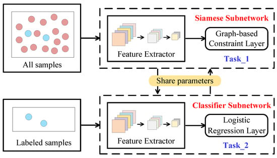
Figure 3.
Deep multitask network.
2.3. Network Architecture and Loss Function of Deep Multitask Network
Figure 4 shows the generation process of training data for DMN. For an HSI dataset, with m samples (labeled and unlabeled) and n labels (). M 3-D cube samples with the spatial neighborhood are first generated. Since the training data of Siamese subnetwork and classifier subnetwork are different, two training sets need to be established. Classifier subnetwork only trains the labeled samples, so its training data contain n 3-D cube samples with labels, as shown in Training Set 1 of Figure 4. In practice, the size of its input is 3-D cube samples . Due to the fact that Siamese subnetwork is to learn the sample relationships in and , in addition to the target sample, nearest neighbors in and farthest neighbors in also need to be input into the network during training. Training Set 2 of Figure 4 are the training data of Siamese subnetwork, which include m training samples , where a training sample contains one target sample , its nearest neighbors from and its farthest neighbors from . It is worth noting that some neighbors of unlabeled samples are labeled samples, which allows the network to learn the relationship between labeled samples and unlabeled samples to promote classification.
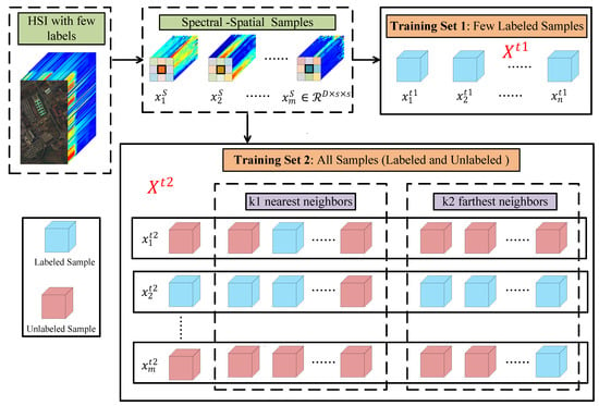
Figure 4.
Generating training data for DMN.
Figure 5 displays the network architecture of classifier subnetwork with a feature extractor and a logistic regression layer. In view of the strong feature extraction capability of convolutional layer, the feature extractor is a fully convolutional network. Here, the features of each layer decrease as the number of layers increases and the size of output is , so the feature extractor can also be regarded as a process of dimensionality reduction. Taking a four-layer feature extractor as an example, for input data , their output can be formulated as
where is the ReLU function and is the 2-D convolution. is the learning parameter of the feature extractor. Feature extractor and logistic regression layer are fully connected. The output of logistic regression layer is formulated as
in which, is the learning parameters of logistic regression layer and is the softmax function. Since the task of classifier subnetwork is classification, for the Training Set 1 , the loss function adopts the cross-entropy loss, which is defined as
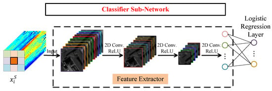
Figure 5.
The network architecture of classifier subnetwork.
Here, is the class label of and is its predicted label. and are two -dimensional one-hot vectors and is the number of classes. is the kth element of and is the kth element of .
The task of Siamese subnetwork is to learn the sample relationships from and . As described in Section 2.2, represents the relationships between the target sample and its nearest neighbors and expresses the relationships between the target sample and its farthest neighbors. In order to learn the graph information in and at the same time, a novel Siamese subnetwork with subnets is designed to learn the relationship between one target sample and samples at a time, of which, the network architecture is shown in Figure 6. This is different from the traditional Siamese network, which has two subnets and only learns the relationship between two samples at a time []. In our designed Siamese network, each subnet has the same network structure as the classifier subnetwork. That is, all subnets have the same network structure with a feature extractor and a graph-based constraint layer. The point is that they share parameters.
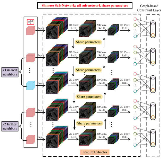
Figure 6.
The network architecture of Siamese subnetwork.
Corresponding to the network architecture, input data of Siamese subnetwork have 3-D cubes and is the target sample. Meanwhile, we suppose that is the pth nearest neighbor of and is the qth farthest neighbor of , which are both 3-D cubes. In Siamese subnetwork, each subnet inputs one 3-D cube . According to the sequence from top to bottom in Figure 6, the first subnet inputs the target sample , and its output can be formulated as
which is same as the output of classifier subnetwork. is also the output of feature extractor and is the learning parameters of graph-based constraint layer. represents a subnet mapping function, which applies to all subnets due to the same network structure and shared parameters. In that way, the second to th subnets input nearest neighbor samples and the th to th subnets input farthest neighbor samples. When a subnet inputs a nearest neighbor of , its output is described as
In the same way, when a subnet inputs a farthest neighbor of , its output is described as
Thus, for input data in Training Set 2 of Figure 4, the output of Siamese subnetwork is
which includes the outputs of subnets. In fact, Siamese subnetwork aims to promote the learning of classifier subnetwork to improve classification performance. As a result, based on and , Siamese subnetwork should compress the distance between the target sample and nearest neighbors and expand the distance between the target sample and farthest neighbors. The former can be formulated as
and the latter can be formulated as
and are the weight matrix from and , respectively, which are calculated with Equations (5) and (7). is based on SLSD, which is proven to be effective in revealing the more real relationships between samples [], where, if SLSD between and is smaller, is larger, and vice versa. Generally, neural networks optimize learning parameters by minimizing objective functions. However, in Siamese subnetwork, needs to be minimized, whereas needs to be maximized. A simple negative optimization will make the network unable to converge. To take into account the convergence of the network, the loss function of Siamese subnetwork is defined as
Here, is a decreasing function and converges to 0 as the variable increases. As a result, the loss function will be optimized towards zero.
2.4. Multitask Few-Shot Learning Strategy
In fact, as its name suggests, DMN is a two-task network. Since the training data required by these two tasks are completely different not only in content but also in format, the learning of DMN faces the problem of the two tasks not being able to update learning parameters in training at the same time. In addition, due to the large difference in the number of training data between the two tasks, DMN learning is easy to fall into a single task, so the two tasks cannot achieve uniform convergence. To sum up, it is challenging to achieve the synergy and balance effect of the two tasks. To solve this problem, we designed a multitask few-shot learning strategy (MFSL).
Next, for ease of explanation, we still introduce MFSL based on two sub-networks. Due to the fact that the purpose of DMN is classification and the number of labeled samples is very small, the learning of the classifier subnetwork is particularly important. The University of Pavia dataset, for example, contains 42,776 samples from nine classes. If five samples are taken from each class, the number of labeled samples is only 45 and the number of unlabeled samples is 42,731. Thus, the number of training samples for the classifier subnetwork is 45, whereas that for the Siamese subnetwork is 42,776, which shows a large gap between them. Therefore, the task of the classifier subnetwork needs to be emphasized constantly.
In this paper, our GDMFSL deals with HSIs with few labels. The training data of the classifier subnetwork of DMN are only labeled samples, so all of them can be used as one batch to participate in DMN learning. Algorithm 1 shows the multitask few-shot learning strategy. MFSL can be understood as that, in training, when the Siamese subnetwork learns a batch of data, the classifier subnetwork also learns a batch of data. When the Siamese subnetwork is learning different batches of data, the classifier subnetwork is always learning a batch of data repeatedly. Of course, when the number of labeled samples increases, the training data of the classifier subnetwork can also be divided into multiple batches. The following experiments also prove that MFSL can balance and converge the two tasks of DMN.
| Algorithm 1: Multitask few-shot learning strategy |
| Input: Training Set 1 with labels, Training Set 2 and its number m, weight matrix and , batch size B, iterations I, learning rate. |
| Initialize: |
| Output: with the input according to Equation (9) |
3. Experiments and Discussion
3.1. Experimental Datasets
To assess the performance of GDMFSL, three public HSI datasets were used, including the Indian Pines (IP), the University of Pavia (UP) and the Salinas.
Figure 7 shows the color image and the labeled image of the IP dataset covering the Indian Pines region, northwest Indiana, USA, which was acquired by the AVIRIS sensor in 1992. Its spatial resolution is 20 m. It has 220 original spectral bands in the wavelength range 0.4∼2.5 . As a result of the noise and water absorption, 104∼108, 150∼163 and 220 spectral bands were abandoned and the remaining 200 bands were used in this paper. It contains pixels, including background with 10,776 pixels and 16 ground-truth classes with 10,249 pixels.

Figure 7.
Indian Pines dataset.
The UP dataset covers the University of Pavia, Northern Italy, which was acquired by the ROSIS sensor. Its spatial resolution is 1.3 m. It has 115 original spectral bands in the wavelength range of 0.4∼0.82 . Due to removing 12 noise bands, 103 bands are employed in this paper. It has pixels, where 164,624 pixels are background and 42,776 pixels are nine ground-truth classes. Figure 8 shows the color image and the labeled image with nine classes.
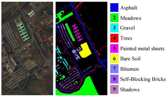
Figure 8.
University of Pavia dataset.
Salinas Dataset covers Salinas Vally, CA, which was acquired by the AVIRIS sensor in 1998. Its spatial resolution is 3.7 m. It has 224 original bands in the wavelength range of 0.4 to 2.45 . Due to the fact that 20 bands are severely affected by noise, the remaining 204 bands are used for this paper. Each band has pixels, including 16 ground-truth classes with 56,975 pixels and background with 54,129 pixels. The color image and the labeled image with 16 classes are shown in Figure 9.
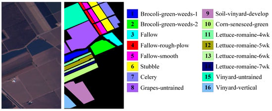
Figure 9.
Salinas dataset.
3.2. Experimental Setting
As described in Section 2.1, our GDMFSL framework consists of two parts: a semi-supervised graph and a deep multitask network. For the semi-supervised graph, four parameters need to be manually set, namely, the size of spatial window s, the spectral–locational trade-off parameter , the number of nearest neighbors and that of farthest neighbors . In fact, the influence of s, and on the graph has been analyzed in []. According to that, these three parameters are set separately for different datasets and is set to be equal to for convenience. In this paper, four parameters were set to , , for the IP dataset, , , for the UP dataset and , , for the Salinas dataset.
Although the DMN contains two subnetworks, their network structure is the same. To further slow down over-fitting and improve DMN classification performance, we added a dropout model between each convolutional layer in the feature extractor. For the IP dataset, the number of features in each layer is , the filter size per layer is , the output size per layer is , the dropout model has a retention probability of 0.9 and the learning rate is . For the UP dataset, the number of features in each layer is , the filter size per layer is , the output size per layer is , the dropout model has a retention probability of 0.9 and the learning rate is . For the Salinas dataset, the number of features in each layer is , the filter size per layer is , the output size per layer is , the dropout model has a retention probability of 0.8 and the learning rate is .
In order to verify the superiority of GDMFSL, eight classification methods are selected for comparison, including SVM, KNN, 3D-CNN [], SSRN [], SS-CNN [], DFSL+NN [], RN-FSC [] and DCFSL []. SVM and KNN are the traditional classification methods and the rest are based on neural networks. In the actual experiment, we utilized the 1-nearest neighbors and a LibSVM toolbox with a radial basis function. 3D-CNN [] and SSRN [] are two supervised 3-D deep learning frameworks. SS-CNN [] is a semi-supervised convolutional neural network. DFSL+NN [], RN-FSC [] and DCFSL [] are three few-shot learning frameworks, all of which are cross-domain methods combined with meta-learning. In the following experiments, 200 labeled source domain samples per class are randomly selected to learn transferable knowledge for these three cross-domain methods.
In order to ensure the fairness of the experiment, 1∼5 labeled target dataset samples per class were used for training, and the rest of the samples of the target dataset were reserved as the testing set. The classification overall accuracy (OA), the average accuracy (AA) and the Kappa coefficient were used to evaluate the classification performance. In addition, each experiment in this paper was repeated 10 times in each condition in order to reduce the experimental random error.
3.3. Convergence Analysis
The DMN in our proposed GDMFSL framework has two subnetworks (tasks) with different loss functions. The classifier subnetwork is used to learn what the sample is, and its loss function is the cross-entropy loss between the outputs of the DMN and labels, which is described in Equation (10). The Siamese subnetwork is used to learn the relationship among samples, and its loss function is the mean-squared loss among outputs of the DMN under different inputs, which compresses the distance between the target samples and its nearest neighbors and expands the distance between the target samples and its farthest neighbors, as described in Equation (17). In addition, the two subnetworks learn under different training data. Meanwhile, they share parameters; that is, they jointly optimize the same learning parameter in the DMN. On the surface, under different directions of optimization, the loss of the two subnetworks is likely to fluctuate, and it is not easy to converge. Nevertheless, to prove the convergence of the two subnetworks of the DMN, we show their loss curves and the classification OA curves of the testing set on three datasets, as shown in Figure 10.
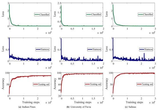
Figure 10.
The loss curves of the DMN and the predicted accuracy of the testing set on three datasets (five labeled samples per class).
The experiment in Figure 10 was performed based on the training data of five labeled samples in each class. The first row is the classifier subnetwork loss, the second row is the Siamese subnetwork loss and the third row is the prediction accuracy of the testing set. Their learning rates are described in Section 3.2. In Figure 10, the x-axis represents the number of learning parameter updates that are performed after learning each batch of samples. The interval within the curve is 100; that is, one loss is recorded for every 100 parameter updates. From Figure 10, the classifier loss of the three datasets has a smooth convergence curve. This proves that, although the amount of training data of the classifier subnetworks is much less than that of the Siamese subnetwork, the task of the classifier subnetwork to learn the labeled samples is not interfered with by the task of the Siamese subnetwork. Though there are fluctuations, the loss curve of the Siamese subnetwork is still gradually converging, which also indicates that our designed loss function in Equation (17) has convergence. These two loss curves also show that the MFSL strategy we designed is also effective. It is worth noting that the prediction accuracy of the test set not only increases gradually with the decrease in the two losses, but also continues to increase with the convergence of the Siamese subnetwork when the classifier subnetwork has converged but the Siamese subnetwork has not. This proves that our designed Siamese subnetwork is quite advantageous for classification.
3.4. Ablation Study
To demonstrate the effectiveness of the strategy proposed in the GDMFSL framework, we conducted an ablation experiment; the results of which are shown in Table 1. Our GDMFSL framework can be divided into two parts: the semi-supervised graph and the DMN. In order to prove the effectiveness of the proposed DMN, we conducted graph learning based on the semi-supervised graph of GDMFSL to reduce the dimensionality of the HSIs dataset, and then classified the dimensionality reduction results using SVM and KNN, which are named SSGL+SVM and SSGL+KNN in this paper. The DMN contains two subnetworks: a classifier subnetwork and a Siamese subnetwork. In order to prove the contribution of the Siamese subnetwork to the DMN, we conducted an experiment to train only the classifier subnetwork, which is called Classifier SubN in Table 1.

Table 1.
Classification accuracy of different methods on three datasets.
Table 1 shows the classification accuracy of SSGL+SVM, SSGL+KNN, Classifier SubN and GDMFSL for three datasets under the condition of a different number of labeled samples, where the highest OA value for the same classification condition has been in bold. GDMFSL, SSGL+SVM and SSGL+KNN learn from the same graph, and the difference is that GDMFSL utilizes DMN to learn not only graph information but also class information, whereas SSGL+SVM and SSGL+KNN only learn graph information. From Table 1, GDMFSL is superior to SSGL+SVM and SSGL+KNN in all conditions on three datasets, which proves that our proposed DMN is effective. In addition, we found that, on the UP dataset, the classification accuracies of SSGL on SVM and KNN are significantly different. This is because the feature extraction and classification in SSGL+SVM and SSGL+KNN are separated, and the feature data distribution of SSGL on the UP dataset is not suitable for the SVM classifier. At this point, a method in which the feature extractor and classifier can learn together is more valuable.
GDMFSL and Classifier SubN are trained with the same labeled samples; the difference is that GDMFSL utilizes the Siamese subnetwork, learning graph information to share the learning parameters to the classifier subnetwork. Table 1 shows that GDMFSL is much better than Classifier SubN, which means that our designed Siamese sub-network is meaningful and can greatly improve the classification performance of the classifier sub-network. Moreover, we can observe from Table 1 that SSGL+SVM and SSGL+KNN are more likely to be better than Classifier SubN. Based on this, it has to be said that the graph-learning method has more advantages than the traditional deep learning method for HSI classification with few labeled samples. The reason for this is that the traditional deep learning method with a deep structure often falls into over-fitting when only few labeled samples are used to train the network. Nevertheless, GDMFSL has solved this problem with the graph, even surpassing the performance of graph learning.
3.5. Classification Result
To further demonstrate the effectiveness of the GDMFSL in HSI classification with few labeled samples, the classification results of GDMFSL and eight comparison methods are presented in this subsection. In the practice experiments, since DFSL+NN [], RN-FSC [] and DCFSL [] are cross-domain methods, four available HSI data sets, Chikusei, Houston, Botswana and Kennedy Space Center, are collected to form source domain data. After discarding classes with less than 200 samples, 40 classes are used to build the source class.
Table 2, Table 3 and Table 4 report the OA, AA, kappa coefficient and the classification accuracy of each class for HSI classification, where the highest value has been in bold. For three target datasets, we randomly selected five labeled samples from each class for training and the rest for testing. In order to eliminate the influence of randomness on the classification accuracy when selecting labeled samples, each experiment was performed 10 times based on an independent randomly labeled sample. From Table 2, Table 3 and Table 4, we obtained the following conclusions.

Table 2.
Classification accuracy (%) of different methods on the IP dataset (five labeled samples per class).

Table 3.
Classification accuracy (%) of different methods on the UP dataset (five labeled samples per class).

Table 4.
Classification accuracy (%) of different methods on the Salinas dataset (five labeled samples per class).
(1) The classification accuracies of deep-learning-based methods are mostly better than those of traditional classification methods. For example, the OA values of 3D-CNN [] and SSRN [] are approximately 13.7% on IP, 8.08% on UP and 5.69% on Salinas higher than those of SVM and KNN, respectively. One reason is that deep learning methods with a hierarchical network structure can obtain more discriminative features. Another reason is that 3D-CNN [] and SSRN [] can obtain spectral–spatial features through the convolutional layer, whereas SVM and KNN only explore spectral features.
(2) Although the learning of unlabeled samples is added in addition to the traditional deep learning method, SS-CNN [], as a semi-supervised method, does not have a better classification performance but is worse when dealing with few labeled sample classification. However, our proposed semi-supervised method, GDMFSL, achieves a good classification performance. The main reason is that SS-CNN [] uses unlabeled samples only for data reconstruction and does not acquire and learn the relationship information among samples.
(3) The few-shot learning methods are superior to the traditional deep-learning-based methods. Numerically, the OA values of DFSL+NN [], RN-FSC [] and DCFSL [] are approximately 3.48% on IP, 9.53% on UP and 1.53% on Salinas higher than those of 3D-CNN [] and SSRN [], respectively. These few-shot learning methods use a meta-learning strategy to learn a metric space suitable for classification. In effect, they are learning a mapping that better expresses the relationships between samples, which is similar to the learning of relationships between samples in our proposed GDMFSL.
(4) Among all of the algorithms, the GDMFSL proposed by us achieved the best classification results on all three data sets. The classification accuracy of GDMFSL is even much higher than other comparison methods. In terms of data, GDMFSL is 20.77% on IP, 2.77% on UP and 9.51% on Salinas higher than the highest OA value in comparison methods. GDMFSL achieved the highest classification accuracy in most classes, with even some classes with a classification accuracy of 100%. In addition, it is worth noting that, in Table 2, when the IP dataset is classified with only five labeled samples in each class, the OA values of all comparison algorithms are all lower than 70%, whereas that of GDMFSL reaches 87.58%. In addition to the OA value, the values of the AA and kappa coefficients of GDMFSL are the highest among all algorithms for the three datasets. All of these can strongly prove the excellent performance of GDMFSL in HSI few-shot classification.
In order to better display and compare the classification results of different methods, we present the classification maps corresponding to Table 2, Table 3 and Table 4, as shown in Figure 11, Figure 12 and Figure 13. Obviously, compared with other comparison methods, the classification map of GDMFSL is the most similar to the ground truth, and the difference in area is the least on the three datasets. Through Figure 11, Figure 12 and Figure 13 the advantages of GDMFSL in processing HSI classification with only few labeled samples are once again proved visually. Although the classification map of GDMFSL looks clear and smooth, GDMFSL still has drawbacks. A careful look at Figure 11, Figure 12 and Figure 13 shows that most of the misclassification pixels of GDMFSL are at the boundary of the class region and are identified as the class of the adjacent region. Meanwhile, the misclassification area is continuous. The reason is that the learning of the DMN in GDMFSL is greatly influenced by sample relationship information generated by a semi-supervised graph based on SLSD with locational information. Although the addition of location information can improve the ability of the DMN to identify samples within the class region, samples at the boundary of the class region are prone to be misclassified.
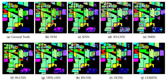
Figure 11.
Classification maps of different methods on the IP dataset.
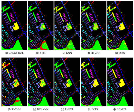
Figure 12.
Classification maps of different methods on the UP dataset.
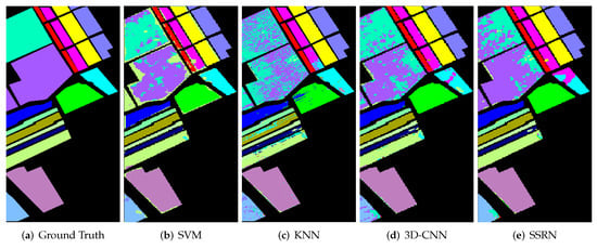
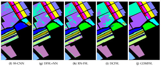
Figure 13.
Classification maps of different methods on the Salinas dataset.
The above experiment shows the five-shot classification performance of GDMFSL for HSIs. In order to further verify the performance of GDMFSL with fewer labeled samples and the effect of a different number of labeled samples on different methods, we randomly selected one, two, three, four and five labeled samples per class for the experiment, of which, the classification OA values are shown in Table 5 in which the highest value has been in bold. To more clearly show the numerical changes and comparison in Table 5, the corresponding line chart is presented in Figure 14. From Table 5 and Figure 14, we obtain the following observations.

Table 5.
Classification accuracy (%) for all methods with different number of labeled sample on three datasets.
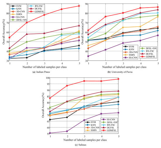
Figure 14.
Classification accuracy for all methods with different number of labeled sample on three datasets.
(1) Though 3D-CNN [] and SSRN [] are superior to SVM and KNN in classification when there are five labeled samples in each class, with the decrease in the number of labeled samples, the advantage of 3D-CNN [] and SSRN [] becomes less and less, and even weaker than SVM and KNN when the number of labeled samples per class is less than three. For example, in the case of one-shot sample classification in the UP dataset, the OA values of SVM and KNN are approximately 6.87% higher than those of 3D-CNN [] and SSRN []. This is because the fewer the training samples, the more serious the overfitting of deep learning methods. DFSL+NN [], RN-FSC [] and DCFSL [] solve this problem through a meta-learning strategy, whereas our GDMFSL learns the relationship among samples from the semi-supervised graph. The experimental results show that, compared with other few-shot learning methods, GDMFSL achieves a better classification performance.
(2) As the number of labeled samples increased, the OA values of all methods increased. When there was only one labeled sample in each class, the OA values of most methods were quite low and close, whereas GDMFSL was the highest, especially on the Salinas dataset, where the OA value of GDMFSL reached 83.52%.
(3) Although the classification performance of SS-CNN [] is relatively weak compared with other methods in this paper, it does not mean that the semi-supervised deep learning method is unreliable. On the contrary, the experimental results of GDMFSL prove that semi-supervised deep learning is quite effective in processing hyperspectral image classification, with a small number of labeled samples when unlabeled samples are reasonably used. Compared with SS-CNN [], GDMFSL has the advantage of learning the relationship among samples.
(4) Obviously, GDMFSL is superior to other few-shot learning methods: DFSL+NN [], RN-FSC [] and DCFSL []. GDMFSL differs from them in that GDMFSL borrows unlabeled sample information from the target dataset whereas they borrow labeled sample information from other source datasets. Objectively speaking, the latter has problems of domain conversion and different classes between different datasets, whereas the former does not.
(5) It is clear from Figure 14 that GDMFSL has the best classification performance under all conditions. Under different numbers of labeled samples, the OA values of GDMFSL are at least 11.29%, 12.18%, 19.46%, 21.12% and 20.77% higher than those of other methods on the IP dataset, 4.35%, 8,35%, 6.18%, 5.12% and 2.77% on the UP dataset and 7.48%, 12.6%, 11.77%, 8.71% and 9.71% on the Salinas dataset.
4. Concluding Remarks
In this paper, we proposed a GDMFSL framework to deal with HSI classification with few labeled training samples. GDMFSL can be viewed as two parts: a semi-supervised graph and a DMN. First, a semi-supervised graph is constructed to generate graph information, which uses SLSD to estimate sample similarities and then revises them with few labeled samples. Second, a DMN with two subnetworks (tasks) is constructed and trained. The classifier subnetwork is trained on few labeled samples, which learns what the sample class is. The Siamese subnetwork is trained based on all samples (labeled and unlabeled), which learns the differences (relationships) among all samples. The loss function constrains the Siamese subnetwork to shorten the distance between the target sample and its nearest (or intra-class) neighbors and widen the distance between the target sample and its farthest (or inter-class) neighbors. The classifier subnetwork and Siamese subnetwork are jointly trained according to the MFSL strategy, and converge cooperatively.
The experimental results demonstrate that our proposed strategy for incorporating graph information into the DNN is more effective than graph learning in handling the few-shot settings of HSIs, the proposed DMN is more efficient than traditional classification networks, our designed Siamese subnetwork indeed alleviates the over-fitting problem of the classifier subnetwork and greatly improves the classification performance, the loss function of the Siamese subnetwork is convergent, and the MFSL strategy is effective for promoting the common convergence of two subnetworks (tasks).
More importantly, GDMFSL is far superior to the other comparison methods in this paper. Under different numbers of labeled samples, the classification OA values of GDMFSL are at least 11.29%, 12.18%, 19.46%, 21.12% and 20.77% higher than those of other methods on the IP dataset, 4.35%, 8.35%, 6.18%, 5.12% and 2.77% on the UP dataset and 7.48%, 12.6%, 11.77%, 8.71% and 9.71% on the Salinas dataset.
The disadvantage of this work is that DMNs with different network structures need to be designed for different datasets, which makes a trained DMN not universal to other data. It can be said that the DMN is overfitting to the target data. Therefore, our future work will focus on improving the generalizability of DMNs.
Author Contributions
Conceptualization, N.L. and J.S.; methodology, N.L.; software, N.L.; validation, N.L., J.S. and X.Z.; formal analysis, N.L.; investigation, N.L.; resources, D.Z.; data curation, N.L. and T.W.; writing—original draft preparation, N.L.; writing—review and editing, N.L.; visualization, N.L.; supervision, D.Z.; project administration, D.Z.; funding acquisition, J.S. and Z.Y. All authors have read and agreed to the published version of the manuscript.
Funding
This work was supported in part by the National Natural Science Foundation of China (Grant No. 62076204), the Postdoctoral Science Foundation of Shannxi Province (Grant No.2017BSHEDZZ77), the China Postdoctoral Science Foundation (Grant nos. 2017M613204 and 2017M623246), and the Postdoctoral Science Foundation of China under Grants 2021M700337.
Data Availability Statement
Not applicable.
Conflicts of Interest
The authors declare no conflict of interest.
Abbreviations
The following abbreviations are used in this manuscript:
| DNN | deep neural network |
| HSI | hyperspectral image |
| GDMFSL | graph-based deep multitask few-shot learning |
| DMN | deep multitask network |
| KNN | K nearest neighbor |
| SVM | support vector machine |
| CNN | convolutional neural network |
| SLSD | spectral-locational-spatial distance |
| MFSL | multitask few-shot learning |
| IP | Indian Pines |
| UP | University of Pavia |
| AVIRIS | Airborne Visible/Infrared Imaging Spectrometer |
| ROSIS | Reflective Optics System Imaging Spectrometer |
| 3D-CNN | 3D convolutional neural network |
| SSRN | spectral–spatial residual network |
| SS-CNN | semi-supervised convolutional neural network |
| DFSL+NN | Deep Few-Shot Learning method with nearest neighbor classifier |
| RN-FSC | relation network for few-shot classification |
| DCFSL | deep cross-domain few-shot learning |
| OA | overall accuracy |
| AA | average accuracy |
| SSGL+SVM | semi-supervised graph learning method with SVM classifier |
| SSGL+KNN | semi-supervised graph learning method with KNN classifier |
References
- ElMasry, G.; Sun, D.W. Principles of hyperspectral imaging technology. In Hyperspectral Imaging for Food Quality Analysis and Control; Elsevier: Amsterdam, The Netherlands, 2010; pp. 3–43. [Google Scholar]
- Boldrini, B.; Kessler, W.; Rebner, K.; Kessler, R.W. Hyperspectral imaging: A review of best practice, performance and pitfalls for in-line and on-line applications. J. Near Infrared Spectrosc. 2012, 20, 483–508. [Google Scholar] [CrossRef]
- Sahoo, R.N.; Ray, S.; Manjunath, K. Hyperspectral remote sensing of agriculture. Curr. Sci. 2015, 108, 848–859. [Google Scholar]
- Bridgelall, R.; Rafert, J.B.; Tolliver, D. Hyperspectral imaging utility for transportation systems. In Sensors and Smart Structures Technologies for Civil, Mechanical, and Aerospace Systems 2015; International Society for Optics and Photonics: Bellingham, WA, USA, 2015; Volume 9435, p. 943522. [Google Scholar]
- Fei, B. Hyperspectral imaging in medical applications. In Data Handling in Science and Technology; Elsevier: Amsterdam, The Netherlands, 2020; Volume 32, pp. 523–565. [Google Scholar]
- Transon, J.; d’Andrimont, R.; Maugnard, A.; Defourny, P. Survey of hyperspectral earth observation applications from space in the sentinel-2 context. Remote Sens. 2018, 10, 157. [Google Scholar] [CrossRef] [Green Version]
- Ding, C.; Li, Y.; Wen, Y.; Zheng, M.; Zhang, L.; Wei, W.; Zhang, Y. Boosting Few-Shot Hyperspectral Image Classification Using Pseudo-Label Learning. Remote Sens. 2021, 13, 3539. [Google Scholar] [CrossRef]
- Chen, Y.; Lin, Z.; Zhao, X.; Wang, G.; Gu, Y. Deep learning-based classification of hyperspectral data. IEEE J. Sel. Top. Appl. Earth Obs. Remote Sens. 2014, 7, 2094–2107. [Google Scholar] [CrossRef]
- Hennessy, A.; Clarke, K.; Lewis, M. Hyperspectral classification of plants: A review of waveband selection generalisability. Remote Sens. 2020, 12, 113. [Google Scholar] [CrossRef] [Green Version]
- Zhang, H.; Li, Y.; Jiang, Y.; Wang, P.; Shen, Q.; Shen, C. Hyperspectral classification based on lightweight 3-D-CNN with transfer learning. IEEE Trans. Geosci. Remote Sens. 2019, 57, 5813–5828. [Google Scholar] [CrossRef] [Green Version]
- Tu, B.; Zhou, C.; He, D.; Huang, S.; Plaza, A. Hyperspectral classification with noisy label detection via superpixel-to-pixel weighting distance. IEEE Trans. Geosci. Remote Sens. 2020, 58, 4116–4131. [Google Scholar] [CrossRef]
- Sawant, S.S.; Prabukumar, M. A review on graph-based semi-supervised learning methods for hyperspectral image classification. Egypt. J. Remote Sens. Space Sci. 2020, 23, 243–248. [Google Scholar] [CrossRef]
- Kang, X.; Xiang, X.; Li, S.; Benediktsson, J.A. PCA-based edge-preserving features for hyperspectral image classification. IEEE Trans. Geosci. Remote Sens. 2017, 55, 7140–7151. [Google Scholar] [CrossRef]
- Bandos, T.V.; Bruzzone, L.; Camps-Valls, G. Classification of hyperspectral images with regularized linear discriminant analysis. IEEE Trans. Geosci. Remote Sens. 2009, 47, 862–873. [Google Scholar] [CrossRef]
- Wang, J.; Chang, C.I. Independent component analysis-based dimensionality reduction with applications in hyperspectral image analysis. IEEE Trans. Geosci. Remote Sens. 2006, 44, 1586–1600. [Google Scholar] [CrossRef]
- He, L.; Li, J.; Plaza, A.; Li, Y. Discriminative low-rank Gabor filtering for spectral–spatial hyperspectral image classification. IEEE Trans. Geosci. Remote Sens. 2016, 55, 1381–1395. [Google Scholar] [CrossRef]
- Zhang, L.; Luo, F. Review on graph learning for dimensionality reduction of hyperspectral image. Geo-Spat. Inf. Sci. 2020, 23, 98–106. [Google Scholar] [CrossRef] [Green Version]
- Tenenbaum, J.B.; De Silva, V.; Langford, J.C. A global geometric framework for nonlinear dimensionality reduction. Science 2000, 290, 2319–2323. [Google Scholar] [CrossRef] [PubMed]
- Fang, Y.; Li, H.; Ma, Y.; Liang, K.; Hu, Y.; Zhang, S.; Wang, H. Dimensionality reduction of hyperspectral images based on robust spatial information using locally linear embedding. IEEE Geosci. Remote Sens. Lett. 2014, 11, 1712–1716. [Google Scholar] [CrossRef]
- Yan, L.; Niu, X. Spectral-angle-based Laplacian eigenmaps for nonlinear dimensionality reduction of hyperspectral imagery. Photogramm. Eng. Remote Sens. 2014, 80, 849–861. [Google Scholar] [CrossRef]
- Zhou, Y.; Peng, J.; Chen, C.P. Dimension reduction using spatial and spectral regularized local discriminant embedding for hyperspectral image classification. IEEE Trans. Geosci. Remote Sens. 2014, 53, 1082–1095. [Google Scholar] [CrossRef]
- Huang, H.; Shi, G.; He, H.; Duan, Y.; Luo, F. Dimensionality reduction of hyperspectral imagery based on spatial–spectral manifold learning. IEEE Trans. Cybern. 2019, 50, 2604–2616. [Google Scholar] [CrossRef] [Green Version]
- Huang, H.; Duan, Y.; He, H.; Shi, G.; Luo, F. Spatial-spectral local discriminant projection for dimensionality reduction of hyperspectral image. ISPRS J. Photogramm. Remote Sens. 2019, 156, 77–93. [Google Scholar] [CrossRef]
- Paoletti, M.; Haut, J.; Plaza, J.; Plaza, A. Deep learning classifiers for hyperspectral imaging: A review. ISPRS J. Photogramm. Remote Sens. 2019, 158, 279–317. [Google Scholar] [CrossRef]
- Li, S.; Song, W.; Fang, L.; Chen, Y.; Ghamisi, P.; Benediktsson, J.A. Deep learning for hyperspectral image classification: An overview. IEEE Trans. Geosci. Remote Sens. 2019, 57, 6690–6709. [Google Scholar] [CrossRef] [Green Version]
- Jiao, L.; Liang, M.; Chen, H.; Yang, S.; Liu, H.; Cao, X. Deep fully convolutional network-based spatial distribution prediction for hyperspectral image classification. IEEE Trans. Geosci. Remote Sens. 2017, 55, 5585–5599. [Google Scholar] [CrossRef]
- Xu, Y.; Du, B.; Zhang, F.; Zhang, L. Hyperspectral image classification via a random patches network. ISPRS J. Photogramm. Remote Sens. 2018, 142, 344–357. [Google Scholar] [CrossRef]
- Zhong, Z.; Li, J.; Luo, Z.; Chapman, M. Spectral–spatial residual network for hyperspectral image classification: A 3-D deep learning framework. IEEE Trans. Geosci. Remote Sens. 2017, 56, 847–858. [Google Scholar] [CrossRef]
- Li, Z.; Huang, H.; Li, Y.; Pan, Y. M3DNet: A manifold-based discriminant feature learning network for hyperspectral imagery. Expert Syst. Appl. 2020, 144, 113089. [Google Scholar] [CrossRef]
- Boggavarapu, L.P.K.; Manoharan, P. A new framework for hyperspectral image classification using Gabor embedded patch based convolution neural network. Infrared Phys. Technol. 2020, 110, 103455. [Google Scholar] [CrossRef]
- Paoletti, M.E.; Haut, J.M.; Plaza, J.; Plaza, A. A new deep convolutional neural network for fast hyperspectral image classification. ISPRS J. Photogramm. Remote Sens. 2018, 145, 120–147. [Google Scholar] [CrossRef]
- Li, N.; Zhou, D.; Shi, J.; Wu, T.; Gong, M. Spectral-locational-spatial manifold learning for hyperspectral images dimensionality reduction. Remote Sens. 2021, 13, 2752. [Google Scholar] [CrossRef]
- Deng, B.; Jia, S.; Shi, D. Deep metric learning-based feature embedding for hyperspectral image classification. IEEE Trans. Geosci. Remote Sens. 2019, 58, 1422–1435. [Google Scholar] [CrossRef]
- Jia, S.; Jiang, S.; Lin, Z.; Li, N.; Yu, S. A Survey: Deep Learning for Hyperspectral Image Classification with Few Labeled Samples. Neurocomputing 2021, 448, 179–204. [Google Scholar] [CrossRef]
- Snell, J.; Swersky, K.; Zemel, R.S. Prototypical Networks for Few-shot Learning. Adv. Neural Inf. Process. Syst. 2017, 30. [Google Scholar]
- Tang, H.; Li, Y.; Han, X.; Huang, Q.; Xie, W. A Spatial–Spectral Prototypical Network for Hyperspectral Remote Sensing Image. IEEE Geosci. Remote Sens. Lett. 2019, 17, 167–171. [Google Scholar] [CrossRef]
- Sung, F.; Yang, Y.; Zhang, L.; Xiang, T.; Torr, P.H.; Hospedales, T.M. Learning to compare: Relation network for few-shot learning. In Proceedings of the IEEE Conference on Computer Vision and Pattern Recognition, Salt Lake City, UT, USA, 18–23 June 2018; pp. 1199–1208. [Google Scholar]
- Gao, K.; Liu, B.; Yu, X.; Qin, J.; Zhang, P.; Tan, X. Deep relation network for hyperspectral image few-shot classification. Remote Sens. 2020, 12, 923. [Google Scholar] [CrossRef] [Green Version]
- Liu, B.; Yu, X.; Zhang, P.; Yu, A.; Fu, Q.; Wei, X. Supervised deep feature extraction for hyperspectral image classification. IEEE Trans. Geosci. Remote Sens. 2017, 56, 1909–1921. [Google Scholar] [CrossRef]
- Wang, W.; Chen, Y.; He, X.; Li, Z. Soft Augmentation-Based Siamese CNN for Hyperspectral Image Classification With Limited Training Samples. IEEE Geosci. Remote Sens. Lett. 2021, 19, 1–5. [Google Scholar] [CrossRef]
- Li, Y.; Zhang, H.; Shen, Q. Spectral–spatial classification of hyperspectral imagery with 3D convolutional neural network. Remote Sens. 2017, 9, 67. [Google Scholar] [CrossRef] [Green Version]
- Liu, B.; Yu, X.; Zhang, P.; Tan, X.; Yu, A.; Xue, Z. A semi-supervised convolutional neural network for hyperspectral image classification. Remote Sens. Lett. 2017, 8, 839–848. [Google Scholar] [CrossRef]
- Liu, B.; Yu, X.; Yu, A.; Zhang, P.; Wan, G.; Wang, R. Deep few-shot learning for hyperspectral image classification. IEEE Trans. Geosci. Remote Sens. 2018, 57, 2290–2304. [Google Scholar] [CrossRef]
- Li, Z.; Liu, M.; Chen, Y.; Xu, Y.; Li, W.; Du, Q. Deep cross-domain few-shot learning for hyperspectral image classification. IEEE Trans. Geosci. Remote Sens. 2021, 60, 1–18. [Google Scholar] [CrossRef]
Publisher’s Note: MDPI stays neutral with regard to jurisdictional claims in published maps and institutional affiliations. |
© 2022 by the authors. Licensee MDPI, Basel, Switzerland. This article is an open access article distributed under the terms and conditions of the Creative Commons Attribution (CC BY) license (https://creativecommons.org/licenses/by/4.0/).