Removing Prior Information from Remotely Sensed Atmospheric Profiles by Wiener Deconvolution Based on the Complete Data Fusion Framework

Abstract

A method is developed that removes a priori information from remotely sensed atmospheric state profiles. This consists of a Wiener deconvolution, whereby the required cost function is obtained from the complete data fusion framework. Asserting that the deconvoluted averaging kernel matrix has to equal the unit matrix, results in an iterative process for determining a profile-specific deconvolution matrix. In contrast with previous deconvolution approaches, only the dimensions of this matrix have to be fixed beforehand, while the iteration process optimizes the vertical grid. This method is applied to ozone profile retrievals from simulated and real measurements co-located with the Izaña ground station. Individual profile deconvolutions yield strong outliers, including negative ozone concentration values, but their spatiotemporal averaging results in prior-free atmospheric state representations that correspond to the initial retrievals within their uncertainty. Averaging deconvoluted profiles thus looks like a viable alternative in the creation of harmonized Level-3 data, avoiding vertical smoothing difference errors and the difficulties that arise with averaged averaging kernels.

1. Introduction

The remote sounding of atmospheric composition and temperature typically involves an under-constrained retrieval process. This process includes a forward model inversion and a cost function minimization, whereby the latter must be converted from an under-constrained problem to a constrained one using external information [1]. The constraining information can either consist of an a priori estimate of the atmospheric state and its covariance, such as in the Optimal Estimation (OE) approach, or a continuity constraint, such as in Philips–Tikhonov-like approaches. In both cases, the resulting retrieved state unavoidably consists of a mixture of information contributed by the measurement and of a priori constraints.

The presence of prior information in the atmospheric state retrievals complicates their scientific application and interpretation in several ways [2]. In comparison with other measured or modeled data, the differences and their uncertainties contain several prior-induced terms that can be hard to estimate [3]. These additional terms not only affect the quantitative validation of remotely sensed data, but also their visual inspection. It is virtually impossible to tell whether significant structures originate from the measurement or from the a priori [2]. Furthermore, depending on the nature of the a priori information, profile retrievals at different locations are no longer statistically independent, which complicates their averaging and assimilation [4,5]. Finally, the data volume of a complete set of diagnostic parameters can be enormous, or users might not deal with this diagnostic information, risking misinterpretation of the data. It is, therefore, often desirable to remove the a priori information from a retrieved product.

Optimal estimation retrievals have the advantage that their information mixing is fully quantified by the retrieval’s averaging kernels [1], represented by a single vector kernel for column retrievals, or by a square averaging kernel matrix for vertically resolved profile retrievals. Consequently, it is, in principle, possible to perform a deconvolution operation that removes the prior information from the retrieval, resulting in a so-called information-centered representation of the retrieved atmospheric state, where each datapoint represents one independent degree of freedom (DOF) [2]. In practice, however, a pure deconvolution is hampered by the presence of the retrieval uncertainty, as expressed by its covariance (matrix).

von Clarmann and Grabowski [2] have nevertheless developed a methodology to convert a given OE profile retrieval into its information-centered representation by imposing a staircase or triangular profile representation. Keppens et al. [3] have later argued that this result can also be obtained from the complete data fusion framework if the latter includes a regridding operation. The complete data fusion framework provides a method for combining retrieved atmospheric states that is equivalent to their simultaneous retrieval [6]. This method, and its ability to combine the replacement of prior information with an interpolation (and a corresponding uncertainty assessment), was developed by Ceccherini et al. [6,7].

In this work, it is demonstrated (next section) that the information-centered representation of a retrieved atmospheric state can also be obtained iteratively by performing a Wiener deconvolution on the retrieved profile. This deconvolution explicitly considers the convoluted state’s uncertainty by minimization of an uncertainty-related cost function [8]. In Section 3, the developed method is applied to a selection of satellite and ground-based atmospheric state retrievals, both from simulated and real data, which are also compared with ozonesonde data to assess the validity of their information-centered representations. The last section provides an additional discussion on the applicability of the developed deconvolution method and conclusions.

2. Methodology

In the absence of uncertainties, an optimal estimation retrieval yields a retrieved profile $\widehat{x}$ given by [1]:

$$\widehat{x}=A{x}_t+\left(I-A\right)x_a$$

(1)

which combines measurement information from the true profile $x_t$ with prior information from the a priori profile $x_a$. The weighting matrix A is called the averaging kernel matrix and is usually non-diagonal, meaning that the elements of the state vector are not mutually independent; I is the unit matrix. As the measurement information from the true profile in terms of the number of degrees of freedom of the retrieval $d\left(\widehat{x}\right)=\mathrm{trace}\left(A\right)$ is typically (much) smaller than the number of retrieved profile levels or layers, both input profiles are strongly convoluted by the averaging kernel matrix A and by $I-A$, respectively. In theory, however, by solving Equation (1) for $x_t$, one can perform a simple deconvolution operation to reconstruct the true profile for a given vertical grid:

$$x_t=A^{-1}\left[\widehat{x}-\left(I-A\right)x_a\right]\equiv A^{-1}{\widehat{x}}^{\prime }$$

(2)

with ${\widehat{x}}^{\prime }=\widehat{x}-\left(I-A\right)x_a$ representing the retrieval after (non-optimized) correction for the prior profile contribution [3].

In reality, the deconvolution operation in Equation (2) is hampered in two ways. First, the under-constrained retrieval typically makes the straightforward inversion of the averaging kernel matrix A impossible. Second, systematic and random uncertainties $ϵ$, originating from both the remote measurement and the retrieval process, contribute to the retrieved profile, resulting in an additional term in Equation (1):

$$\widehat{x}=A{x}_t+\left(I-A\right)x_a+ϵ$$

(3)

and making the solution for $x_t$ undetermined by a term $A^{-1}ϵ$ that includes contributions from the chosen a priori and its constraints. In order to obtain a direct estimate $x=〈x_t〉$ of the true profile in the absence of prior information, i.e., obtain an information-centered representation of $\widehat{x}$, one needs a different approach.

von Clarmann and Grabowski [2] make use of the Optimal Estimation retrieval theory developed by Rodgers [1] to combine a prior replacement operation with a vertical regridding operation:

$$x=W\left[{\left(S_x^{-1}-S_a^{-1}+S_a^{\prime -1}\right)}^{-1}\left(S_x^{-1}\widehat{x}-S_a^{-1}{x}_a+S_a^{\prime -1}{x}_a^{\prime }\right)\right]$$

(4)

with $S_x$ representing the retrieval covariance matrix associated with $ϵ$(thus omitting the vertical smoothing error covariance because of the subsequent regridding operation; see the end of this section). $x_a^{\prime }$ and $S_a^{\prime }$ are the new prior profile and prior covariance matrix of choice, respectively, that have to replace the retrieval’s initial $x_a$ and $S_a$. The regridding matrix W converts the vertical grid z of $\widehat{x}$ to $z^{\prime }=Wz$ of x. The information-centered representation of $\widehat{x}$ is the one that defines W, $x_a^{\prime }$ and $S_a^{\prime }$ in such a way that x no longer contains any prior information. This is achieved by setting $x_a^{\prime }=0$ and determining the matrices W and $S_a^{\prime }$ that satisfy $W^{*T}{S}_a^{\prime -1}{W}^{*}=0$ non-trivially, with $W^{*}={\left(W^{T}W\right)}^{-1}{W}^T$ being the least-squares pseudo-inverse of W. von Clarmann and Grabowski [2] provide two approaches for this, using either a staircase or triangular representation of $S_a^{\prime -1}$.

In this work, we present an alternative approach using a Wiener deconvolution in the vertical domain that minimizes an uncertainty-related cost function [8]. Based on [1], the required cost function $c\left(x\right)$ was developed within the complete data fusion framework [6]:

$$c\left(x\right)={\left({\widehat{x}}^{\prime }-Ax\right)}^T{S}_x^{-1}\left({\widehat{x}}^{\prime }-Ax\right)+{\left(x-x_a^{\prime }\right)}^T{S}_a^{\prime -1}\left(x-x_a^{\prime }\right)$$

(5)

with $x_a^{\prime }$ and $S_a^{\prime }$ the new prior profile and prior covariance matrix that constrain the solution of the cost function minimization (and note the use of ${\widehat{x}}^{\prime }$, as defined in Equation (2), instead of $\widehat{x}$). In contrast with Equation (4), however, $x_a^{\prime }$ and $S_a^{\prime }$ can immediately be defined on a different vertical grid than the initial retrieval $\widehat{x}$. In that case, it suffices to replace both terms $Ax$ by $A{W}^{*}x$ in Equation (5). Minimizing $c\left(x\right)$ then yields [7]:

$$x={\left(W^{*T}{A}^T{S}_x^{-1}A{W}^{*}+S_a^{\prime -1}\right)}^{-1}\left(W^{*T}{A}^T{S}_x^{-1}{\widehat{x}}^{\prime }+S_a^{\prime -1}{x}_a^{\prime }\right)$$

(6)

The constraint $S_a^{\prime -1}=0$ on the new vertical grid can hence be straightforwardly imposed within the complete data fusion framework. Insertion in Equation (6) results in:

$$x={\left(W^{*T}{A}^T{S}_x^{-1}A{W}^{*}\right)}^{-1}{W}^{*T}{A}^T{S}_x^{-1}{\widehat{x}}^{\prime }\equiv P{\widehat{x}}^{\prime }$$

(7)

with $P={\left(W^{*T}{A}^T{S}_x^{-1}A{W}^{*}\right)}^{-1}{W}^{*T}{A}^T{S}_x^{-1}$. The latter identification demonstrates that Equation (7) can still be considered a deconvolution with $A^{-1}$ in Equation (2) being replaced by a Wiener-like deconvolution matrix P that also includes a regridding operation. P equals the least-squares inverse of $A{W}^{*}$ if $S_x^{-1}=I$.

Equation (7) is mathematically equivalent to Equation (4) with $W^{*T}{S}_a^{\prime -1}{W}^{*}=0$ [3], but has the important advantage that only W has to be determined. This can be carried out quite straightforwardly from the observation that the averaging kernel matrix of the information-centered representation has to equal the unit matrix. The averaging kernel matrix $A^{\prime }$ that corresponds with x is given by the application of the deconvolution P to $A{W}^{*}$ or $A^{\prime }=PA{W}^{*}$ [3,7]. Within the complete data fusion framework, the information-centered representation thus depends on obtaining a regridding matrix $W^{*}$ that fulfills

$$A^{\prime }=PA{W}^{*}={\left(W^{*T}{A}^T{S}_x^{-1}A{W}^{*}\right)}^{-1}{W}^{*T}{A}^T{S}_x^{-1}A{W}^{*}=I$$

(8)

by construction, or $W=PA$. One, hence, immediately obtains an analytical yet recursive expression for the looked-after regridding matrix W:

$$W={\left(W^{*T}{A}^T{S}_x^{-1}A{W}^{*}\right)}^{-1}{W}^{*T}{A}^T{S}_x^{-1}A$$

(9)

which cannot be trivially solved for W, as even its dimensions are undetermined. However, considering that $PA{W}^{*}$ has to reproduce the unit matrix, one can preset the dimensions of W by $\dim \left(W\right)=(d,\dim \left(\widehat{x}\right))$, with d being the rounding of the number of degrees of freedom of the initial retrieval (although this number slightly depends on the retrieval constraints; see the next section).

Fixing the dimensions of W, Equation (9) can easily be iteratively solved, e.g., one can opt for a pseudo-inverse linear or mass-conserving regridding [3,9] from the initial retrieval grid towards d equidistant levels spanning the same vertical range as a first estimate $W_0$, and hence apply:

$$W_{i+1}={\left(W_i^{*T}{A}^T{S}_x^{-1}A{W}_i^{*}\right)}^{-1}{W}_i^{*T}{A}^T{S}_x^{-1}A$$

(10)

until a converged solution of Equation (9) is reached within a given limit. As such, apart from its number of elements, the vertical target grid $z^{\prime }$ is optimally determined by the iteration process and must not be assumed to be a subset of the initial vertical retrieval grid z, as in the approach developed by von Clarmann and Grabowski [2]. The deconvoluted profile $x=P{\widehat{x}}^{\prime }=W{A}^{*}{\widehat{x}}^{\prime }$ on $z^{\prime }=Wz$ and the corresponding covariance matrix $S_x^{\prime }=P{S}_x{P}^T$ immediately follow from [3], while $A^{\prime }\equiv I$ by construction.

The vertical smoothing difference error [2,3] or vertical interpolation error [7] introduced by combining the deconvolution operation with a regridding operation equals $(A-WA)S_A{(A-WA)}^T$ on the initial vertical retrieval grid z, provided that the covariance matrix $S_A$ of choice fully characterizes the true atmospheric variability [2,3,7]. This uncertainty contribution however disappears when represented on the coarser grid $z^{\prime }$ of the deconvoluted profile x if the atmospheric variability is still sufficiently well-characterized by $S_A^{\prime }=W{S}_A{W}^T$ [2]. This condition is assumed to be fulfilled in the following, with $S_x^{\prime }$ thus representing the full ex-ante uncertainty on x.

3. Demonstrative Application

3.1. Settings

Several approaches can be considered to determine the regridding matrix $W_0$ that serves as a first guess in the iterative method outlined above. In the approach presented here, the dimensions of W are preset by $\dim \left(W\right)=(d,\dim \left(\widehat{x}\right))$, with d the rounding of the number of degrees of freedom of the initial retrieval. This rounding is performed towards either the upper (U) integer $d+={\mathrm{int}}_U\left(\mathrm{trace}\left(A\right)\right)$ or the lower (L) integer $d-={\mathrm{int}}_L\left(\mathrm{trace}\left(A\right)\right)$; see

Table 1. Definition of the rounded number of degrees of freedom of a retrieval d and the initial guess $z_0^{\prime }$ for the vertical levels or layers of the information-centered representation, with k going from 0 to $d-1$ for level representations, and from 0 to $d-2$ for layer representations.

	Levels	Layers
$d+$	$d={\mathrm{int}}_U\left(\mathrm{trace}\left(A\right)\right)$ $z_0^{\prime }=z\left(1\right)+k\Delta z/(d-1)$	/
$d-$	$d={\mathrm{int}}_L\left(\mathrm{trace}\left(A\right)\right)$ $z_0^{\prime }=z\left(1\right)+k\Delta z/(d-1)$	$d={\mathrm{int}}_U\left(\mathrm{trace}\left(A\right)\right)$ $z_0^{\prime }=z\left(1\right)+(k+1/2)\Delta z/(d-1)$

. $W_0$ is then determined as a regridding matrix from the vertical grid z of $\widehat{x}$ to the first guess $z_0^{\prime }$ of the information-centered grid, such that $z_0^{\prime }=W_{0}z$ [3]. In this work, $z_0^{\prime }$ was defined by $d+$ or $d-$ equidistant levels (keeping the upper and lower level of z; see Table 1, first column), or $d-$ equidistant layer centers in between $d+$ levels (see Table 1, second column). Other choices could be made, e.g., based on the staircase or triangular representation by von Clarmann and Grabowski [2], but the iterative process that follows automatically shifts the levels or layer centers to their optimal deconvoluted positions, i.e., the positions with the most retrieval information. Finally, as $z_0^{\prime }$ is coarser than z, $W_0$ was defined as a pseudo-inverse linear interpolation matrix [3]. The maximum number of iterations using Equation (10) was set to 100 for all deconvolutions, but convergence is typically reached after about 10 to 20 iterations. The deconvoluted profile was calculated by use of Equation (7) immediately afterwards.

3.2. Simulated Data

The profile retrieval deconvolution method outlined above was first applied to the ozone data retrieved from spectra that were simulated from a known ’true’ atmospheric state. Such retrievals were generated within the H2020 project Advanced UV Radiation and Ozone Retrieval for Applications (AURORA) to assess the effect of complete data fusion when preceding data assimilation experiments [10]. Using NASA’s MERRA-2 re-analysis of ozone as true atmospheric state, ozone profile data were retrieved from the simulated spectra of the future Copernicus Sentinel-5 UVNS ultraviolet-visible (UV-VIS) and IASI-NG thermal infrared (TIR) nadir spectrometers that will be launched in 2024 on board the EUMETSAT Metop-SG-A1 polar satellite. In this work, we consider the satellite ozone profile retrievals of April 2012 within a 50 km radius of the NDACC ground-based station of Izaña. These have an average DOF of 6.5 and 5.0, respectively, while most retrieval levels show an error e (square root of the retrieval covariance matrix diagonal) of about $0.1\times {10}^{12}$ molecules/cm³ (see

Table 2. Data specifications for the six demonstrative datasets (April 2012): data source, data version, maximum co-location distance from Izaña (in km), number of co-located profiles, average number of independent degrees of freedom d, and average retrieval error e around the ozone maximum and in the troposphere (in ${10}^{12}$ molecules/cm³). Top two rows specify simulated data for the Metop-SG-A1 UVNS and IASI-NG instruments; bottom four rows specify real observations acquired by the NDACC FTIR instrument operating at Izaña and by three different satellite sounders.

Data Source	Data Version	Coinc.	Profs.	Avg. d	Avg. e
S5 UVNS sim. UV	AURORA [10]	50	67	6.5	0.1–0.1
IASI-NG sim. TIR	AURORA [10]	50	46	5.0	0.1–0.1
FTIR spectrometer	NDACC [11]	/	22	4.2	0.4–0.1
IASI on Metop-A	FORLI v2015 [12]	30	28	3.4	0.2–0.2
GOME-2 on Metop-A	RAL v2.14 [13]	100	27	5.6	0.2–0.6
MIPAS on Envisat	ORM v8.22 [14]	500	7	23.2	0.1–0.3

).

From Figure 1, it becomes clear that equating the number of deconvolution levels with the upper integer $d+$ (from 5 to 7 in this case) of the retrieval’s DOF introduces largely deviating profile values where the retrieval sensitivity is low (level’s degrees of freedom ≪1). This is due to the sub-optimal deconvolution process in the presence of the remaining prior information, which is forced into the deconvoluted profile, as $d+$ is larger than d. Setting the number of deconvolution levels to $d-$ (4 to 6 here), i.e., the lower integer of the retrieval’s DOF, resolves this issue, resulting in deconvoluted profiles that can mostly be found within the retrieval error (last column of Table 2) from the retrieved profile. However, part of the retrieval information (less than one DOF by definition) is unavoidably lost as a result, which might, together with the absence of prior information, partially explain the remaining presence of some deviating deconvoluted ozone concentrations, especially near the surface.

In Figure 1, it is shown that attributing the deconvoluted profile’s elements to either $d-$ levels or $d-$ layers does make a difference (middle and bottom panels, respectively). For the UVNS and IASI-NG simulated retrievals, the layer representation yields improved results with respect to the level representation—in terms of closeness to the ’true’ MERRA-2 profile—for the UV data, while the opposite is true for the TIR data. This might be due to the fact that the TIR retrieval obtains more information near the surface, which is better represented in the (surface) level representation than in the (tropospheric) layer representation (and vice versa for the UV data). In the next section, however, which considers real data, this distinction becomes less pronounced for the infrared retrievals with lower DOF.

3.3. Real Observations

Ozone profile data based on real observations were acquired from four instruments and compared with the corresponding deconvoluted profiles in Figure 2. The observations originate from the FTIR spectrometer operated at Izaña (Tenerife Island, 28.3° N, 16.5° W, 2390 m a.s.l.) in the framework of the Network for the Detection of Atmospheric Composition Change (NDACC), and from three different satellite instruments that regularly overpassed Izaña in April 2012 (see Table 2). The GOME-2 and IASI instruments on the EUMETSAT Metop-A platform—hereafter GOME-2A and IASI-A—provided nadir UV and TIR measurements, respectively [12,13], while the Michelson Interferometer for Passive Atmospheric Sounding (MIPAS) on ESA’s Envisat platform measured infrared limb emission spectra in the middle and upper atmosphere [15].

Homogenised FTIR ozone profile data were collected through the NDACC Data Host Facility (DHF) [11]. Ozone profile retrievals from the satellite spectrometers were collected through ESA’s Climate Change Initiative project on Ozone. The Fast Optimal Retrieval on Layers for IASI (FORLI) v20151001 and the Rutherford Appleton Laboratory (RAL) GOME-type ozone profile retrieval v2.14 were thoroughly validated within this project [16]. The MIPAS-Optimised Retrieval Model (ORM) version 8.22 was developed and evaluated within the instrument-specific Quality Working Group [14]. Note that MIPAS data for April 2012 actually cover about one week of soundings only, as contact with the Envisat satellite was lost on April 8 that year.

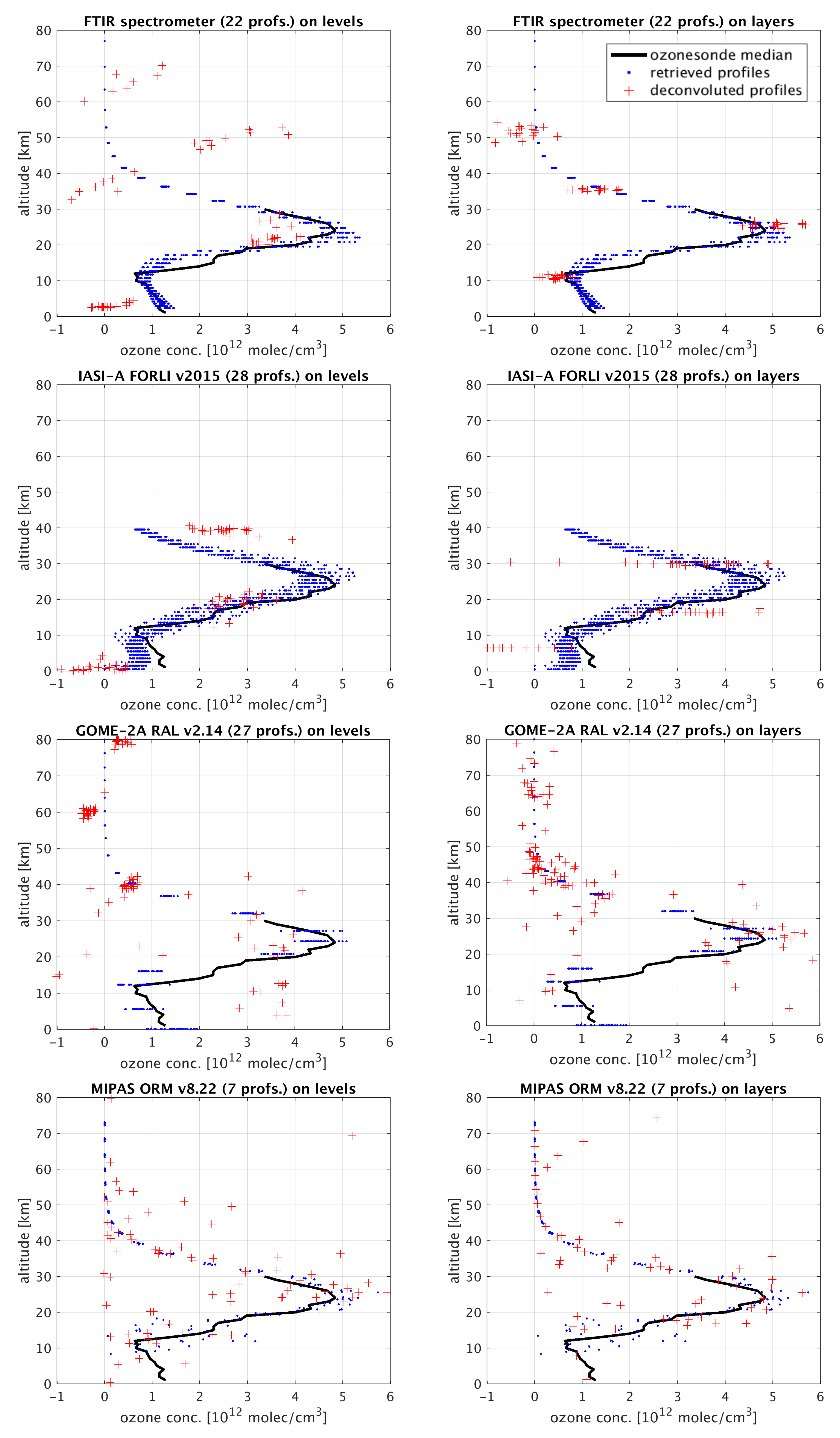
Figure 2 displays the ozone profile retrievals and corresponding deconvoluted profiles from all four instruments, together with the median value of the ozone profile measured at Izaña by balloon-borne ozonesondes as a mutual reference (four weekly launches in April 2012 obtained from the NDACC DHF) [17]. Deconvolutions are performed both for $d-$ levels and for the same amount of layers. The two approaches yield realistic deconvoluted profile results for all four instruments, although strong outliers occur (values deviating from the initial retrieval largely beyond the retrieval error displayed in Table 2), including negative ozone concentrations. These negative values can be set to zero for individual profile deconvolutions, but are better maintained when calculating averages, as demonstrated in the next section.

Although the level and layer deconvolution representations yield quite similar results, the amount of outliers is somewhat smaller in the latter. Moreover, the layer centers seem to be more vertically redistributed by the iterative deconvolution process compared to the individual levels. These small differences are most apparent in the troposphere and towards the higher stratosphere, where ozone values are low in comparison with the stratospheric ozone layer.

The tropospheric ozone amount remains difficult to retrieve, although the FTIR instrument captures the ozone minimum around 10 km very well in its layer-based representation. For the space-based nadir instrument GOME-2A, however, the lowest deconvoluted level or layer is often shifted towards higher altitudes, due to a lack of retrieval information, i.e., sensitivity in the averaging kernels, below the tropopause. On the other hand, some MIPAS limb retrieval deconvolutions iteratively position the lowest level or layer outside of the instrument’s field of view (below about 10 km).

3.4. Retrieval Averaging

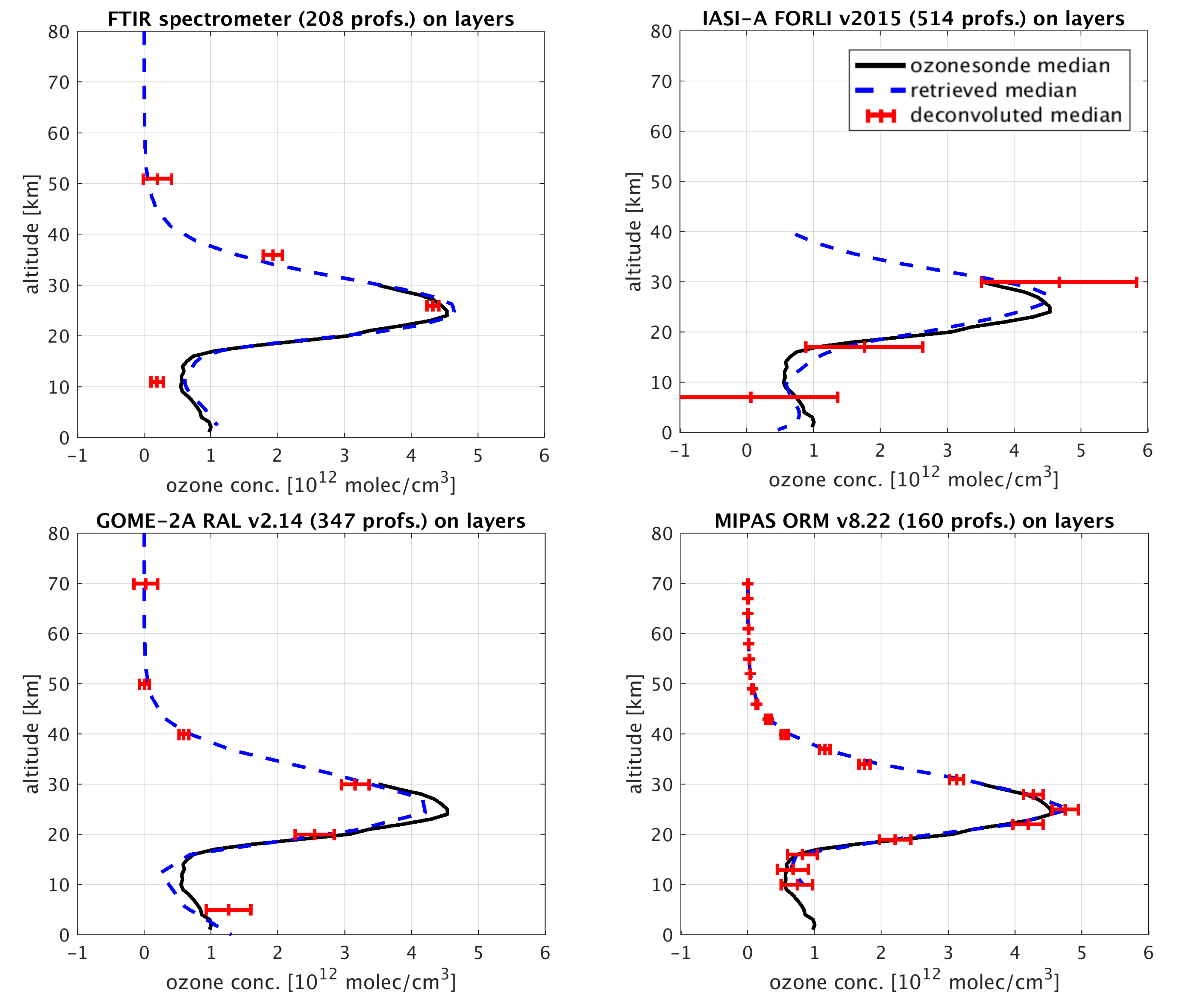
While Figure 2 indicates that individual deconvoluted profiles are not typically suitable for spatiotemporally detailed studies of the atmospheric state, their averaging might yield more useful results. An example is provided in Figure 3, showing median retrieved and deconvoluted profiles for the four aforementioned instruments in 2010, again collocated with the Izaña station (using the same coincidence criteria as in Table 2). Deconvolutions are performed for $d-$ layers and linearly resampled to a common vertical grid with the same number of elements (at rounded median altitudes) before averaging. The median ozonesonde profile for 2010 (51 launches) is added as a mutual reference.

The error bars b that are added to the median deconvoluted profiles represent two ex-ante standard deviations, as calculated from the median deconvoluted covariance matrix diagonal (thus not representing the dispersion around the median): $b\left(i\right)=2{〈S_x^{\prime }(i,i)〉}^{1/2}$ at layer i, with angle brackets for the median here. As such, they show the full estimated retrieval uncertainty at the $95\%$ interval for the median deconvoluted profile, including the (median) vertical smoothing difference error (see Section 2).

It is quite clear from Figure 3 that the averaging of deconvoluted profiles can yield prior-free atmospheric state representations that correspond with the initial retrievals within their uncertainty, although the tropospheric ozone concentration remains an issue for the examples shown here. For the retrievals with a sufficient DOF, e.g., more than 5 like the nadir UV and limb retrievals, deconvoluted profiles are a viable alternative in the creation of spatiotemporally averaged (Level-3) data, thus avoiding smoothing difference errors and the difficulties that arise in the need for and application of averaged averaging kernels [4,5].

4. Conclusions

This work explores and develops a novel method for obtaining an information-centered representation, stripped of all a priori constraint information, of an optimally estimated atmospheric state. The method basically consists of a Wiener deconvolution of the retrieved atmospheric profile, which considers the convoluted state’s uncertainty by minimization of a cost function. The required cost function was taken from the complete data fusion framework, by setting its converted prior constraint to zero ($S_a^{\prime -1}=0$). Additionally asserting that the deconvoluted averaging kernel matrix has to equal the unit matrix results in an iterative procedure for determining the deconvolution matrix P. In contrast with previous approaches, this iteration process automatically shifts the levels or layers of the information-centered profile to their optimal deconvoluted positions, i.e., where most of the retrieval information is.

This deconvolution method has been demonstratively applied to simulated ozone retrievals and to real ozone profile observations at the Izaña ground station in April 2012. The simulated Metop-SG-A1 UVNS (Sentinel-5) and IASI-NG TIR retrievals revealed the necessity of presetting the number of deconvolution levels or layers to the lower integer of each retrieval’s degrees of freedom. This approach results in some loss of retrieved information (less than one DOF), but it also avoids strong prior-induced fluctuations in the deconvoluted profiles. The deconvolution of real FTIR, GOME-2A, IASI-A, and MIPAS ozone profile observations at Izaña confirmed that individual deconvoluted profiles often largely deviate from their initial retrievals. This is an expected result; there is a reason for the insertion of a priori information (as a retrieval constraint) in the first place. The number of outliers seems to be slightly reduced in the layer representation of the deconvoluted profiles with respect to their level representation, but negative ozone concentrations still occur outside of the stratospheric ozone layer.

It is, therefore, suggested to rather apply a deconvolution process upon the creation of spatiotemporally averaged (Level-3-like) data. Although resampling to a common vertical grid is required, the preceding retrieval deconvolution avoids smoothing difference errors and difficulties with averaged averaging kernels. However, if the retrieval DOF or the number of profiles to be averaged is low (e.g., below 5 and about 50, respectively), it might be necessary to reinsert common prior information in the averaged profile. Doing this essentially comes down to the application of the complete data fusion framework for data harmonization, while this work exploits its limiting case for $S_a^{\prime -1}=0$ (cf. Section 2). Both options are being currently considered by the authors in their contributions to the Committee on Earth Observation Satellites (CEOS) tropospheric ozone activity (VC-20-01: Tropospheric Ozone Dataset Validation and Harmonization) and to the second phase of the Tropospheric Ozone Assessment Report (TOAR-II, 2020–2024) of the International Global Atmospheric Chemistry (IGAC) project. Some of the data harmonization shortcomings revealed in the first phase of TOAR (2014–2019) are, hence, explicitly addressed [18].

References

1. Rodgers, C.D. Inverse Methods for Atmospheric Sounding: Theory and Practice; World Scientific: Singapore, 2000. [Google Scholar]
2. von Clarmann, T.; Grabowski, U. Elimination of hidden a priori information from remotely sensed profile data. Atmos. Chem. Phys. 2007, 7, 397–408. [Google Scholar] [CrossRef] [Green Version]
3. Keppens, A.; Compernolle, S.; Verhoelst, T.; Hubert, D.; Lambert, J.C. Harmonization and comparison of vertically resolved atmospheric state observations: Methods, effects, and uncertainty budget. Atmos. Meas. Tech. 2019, 12, 4379–4391. [Google Scholar] [CrossRef] [Green Version]
4. Ceccherini, S.; Carli, B.; Raspollini, P. The average of atmospheric vertical profiles. Opt. Express 2014, 22, 24808–24816. [Google Scholar] [CrossRef] [PubMed]
5. von Clarmann, T.; Glatthor, N. The application of mean averaging kernels to mean trace gas distributions. Atmos. Meas. Tech. 2019, 12, 5155–5160. [Google Scholar] [CrossRef] [Green Version]
6. Ceccherini, S.; Carli, B.; Raspollini, P. Equivalence of data fusion and simultaneous retrieval. Opt. Express 2015, 23, 8476–8488. [Google Scholar] [CrossRef] [PubMed]
7. Ceccherini, S.; Carli, B.; Tirelli, C.; Zoppetti, N.; Del Bianco, S.; Cortesi, U.; Kujanpää, J.; Dragani, R. Importance of interpolation and coincidence errors in data fusion. Atmos. Meas. Tech. 2018, 11, 1009–1017. [Google Scholar] [CrossRef] [Green Version]
8. Wiener, N. Extrapolation, Interpolation, and Smoothing of Stationary Time Series; Wiley: New York, NY, USA, 1949. [Google Scholar]
9. Langerock, B.; De Mazière, M.; Hendrick, F.; Vigouroux, C.; Desmet, F.; Dils, B.; Niemeijer, S. Description of algorithms for co-locating and comparing gridded model data with remote-sensing observations. Geosci. Model Dev. 2015, 8, 911–921. [Google Scholar] [CrossRef] [Green Version]
10. Cortesi, U.; Ceccherini, S.; Del Bianco, S.; Gai, M.; Tirelli, C.; Zoppetti, N.; Barbara, F.; Bonazountas, M.; Argyridis, A.; Bós, A.; et al. Advanced Ultraviolet Radiation and Ozone Retrieval for Applications (AURORA): A Project Overview. Atmosphere 2018, 9, 454. [Google Scholar] [CrossRef] [Green Version]
11. García, O.E.; Schneider, M.; Sepúlveda, E.; Hase, F.; Blumenstock, T.; Cuevas, E.; Ramos, R.; Gross, J.; Barthlott, S.; Röhling, A.N.; et al. Twenty years of ground-based NDACC FTIR spectrometry at Izaña Observator—Overview and long-term comparison to other techniques. Atmos. Chem. Phys. Discuss. 2021, 2021, 15519–15554. [Google Scholar] [CrossRef]
12. Hurtmans, D.; Coheur, P.F.; Wespes, C.; Clarisse, L.; Scharf, O.; Clerbaux, C.; Hadji-Lazaro, J.; George, M.; Turquety, S. FORLI radiative transfer and retrieval code for IASI. J. Quant. Spectrosc. Radiat. Transf. 2012, 113, 1391–1408. [Google Scholar] [CrossRef]
13. Miles, G.M.; Siddans, R.; Kerridge, B.J.; Latter, B.G.; Richards, N.A.D. Tropospheric ozone and ozone profiles retrieved from GOME-2 and their validation. Atmos. Meas. Tech. 2015, 8, 385–398. [Google Scholar] [CrossRef] [Green Version]
14. Raspollini, P.; Piro, A.; Hubert, D.; Keppens, A.; Lambert, J.C.; Wetzel, G.; Moore, D.; Ceccherini, S.; Gai, M.; Barbara, F.; et al. ENVIromental SATellite (ENVISAT) Michelson Interferometer for Passive Atmospheric Sounding (MIPAS) ESA Level 2 Version 8.22 Products—Product Quality Readme File; Technical Report; ESA: Paris, France, 2020; Available online: https://earth.esa.int/eogateway/documents/20142/37627/README_V8_issue_1.0_20201221.pdf (accessed on 24 March 2022).
15. Fischer, H.; Birk, M.; Blom, C.; Carli, B.; Carlotti, M.; von Clarmann, T.; Delbouille, L.; Dudhia, A.; Ehhalt, D.; Endemann, M.; et al. MIPAS: An instrument for atmospheric and climate research. Atmos. Chem. Phys. 2008, 8, 2151–2188. [Google Scholar] [CrossRef] [Green Version]
16. Keppens, A.; Lambert, J.C.; Granville, J.; Hubert, D.; Verhoelst, T.; Compernolle, S.; Latter, B.; Kerridge, B.; Siddans, R.; Boynard, A.; et al. Quality assessment of the Ozone_cci Climate Research Data Package (release 2017)—Part 2: Ground-based validation of nadir ozone profile data products. Atmos. Meas. Tech. 2018, 11, 3769–3800. [Google Scholar] [CrossRef] [Green Version]
17. Schneider, M.; Blumenstock, T.; Hase, F.; Höpfner, M.; Cuevas, E.; Redondas, A.; Sancho, J. Ozone profiles and total column amounts derived at Izaña, Tenerife Island, from FTIR solar absorption spectra, and its validation by an intercomparison to ECC-sonde and Brewer spectrometer measurements. J. Quant. Spectrosc. Radiat. Transf. 2005, 91, 245–274. [Google Scholar] [CrossRef]
18. Gaudel, A.; Cooper, O.R.; Ancellet, G.; Barret, B.; Boynard, A.; Burrows, J.P.; Clerbaux, C.; Coheur, P.F.; Cuesta, J.; Cuevas, E.; et al. Tropospheric Ozone Assessment Report: Present-day distribution and trends of tropospheric ozone relevant to climate and global atmospheric chemistry model evaluation. Elem. Sci. Anth. 2018, 6, 39. [Google Scholar] [CrossRef]
Figure 1. Metop-SG-A1 simulated ozone profile retrievals (blue dots) and deconvoluted profiles (red crosses) from the Sentinel-5 UV (left) and IASI-NG TIR (right) spectral bands for April 2012 and within 50 km of Izaña. Either the upper ( d + , top) or lower ( d , middle and bottom) nearest integer of the initial number of retrieval degrees of freedom determines the number of elements in the deconvoluted profile. In the middle panels, these elements are attributed to d levels, while in the bottom panels, they are attributed to d layers. Grey lines show the ’true’ ozone profile as the median of MERRA-2 within the same spatiotemporal domain.
Remotesensing 14 02197 g001
Figure 2. Ozone profile retrievals (blue dots) and deconvoluted ozone profiles (red crosses) from the NDACC FTIR, IASI-A, GOME-2A, and MIPAS instruments (top to bottom) for April 2012 at Izaña (see coincidence criteria in Table 2). Deconvolutions are performed for d levels (left) or layers (right). Black lines show the median of the ozone profiles measured by ozonesonde at Izaña (4 launches in April 2012).
Remotesensing 14 02197 g002
Figure 3. Yearly median ozone profile retrievals (blue dashes) and deconvoluted profiles (red crosses) from the NDACC FTIR, IASI-A, GOME-2A, and MIPAS instruments (left to right and top to bottom) for 2010 at Izaña (see coincidence criteria in Table 2). Deconvolutions are performed for d layers. Horizontal error bars represent two ex-ante standard deviations, as calculated from the median deconvoluted covariance matrix diagonal (see main text). Black lines show the median of the ozone profiles measured by ozonesonde at Izaña (51 launches in 2010).
Remotesensing 14 02197 g003