Article

Characterizing Spatiotemporal Variations in the Urban Thermal Environment Related to Land Cover Changes in Karachi, Pakistan, from 2000 to 2020

1
Key Laboratory of Digital Earth Science, Aerospace Information Research Institute, Chinese Academy of Sciences, Beijing 100094, China
2
University of Chinese Academy of Science, Beijing 100049, China
3
International Research Center of Big Data for Sustainable Development Goals, Beijing 100094, China
4
Dawn GIS, Geospatial Statistical Research & Analysis Division, Karachi 75300, Pakistan
5
State Key Laboratory of Information Engineering in Surveying, Mapping and Remote Sensing (LIESMARS), Wuhan University, Wuhan 430079, China
6
Institute of Geography, Humboldt University of Berlin, 12489 Berlin, Germany
7
Airborne Remote Sensing Center, Aerospace Information Research Institute, Chinese Academy of Sciences, Beijing 100094, China
*
Author to whom correspondence should be addressed.
Remote Sens. 2022, 14(9), 2164; https://doi.org/10.3390/rs14092164
Submission received: 30 March 2022 / Revised: 26 April 2022 / Accepted: 26 April 2022 / Published: 30 April 2022
(This article belongs to the Special Issue Remote Sensing-Based Urban Morphology Analysis)

Abstract

:
Understanding the spatiotemporal patterns of urban heat islands and the factors that influence this phenomenon can help to alleviate the heat stress exacerbated by urban warming and strengthen heat-related urban resilience, thereby contributing to the achievement of the United Nations Sustainable Development Goals. The association between surface urban heat island (SUHI) effects and land use/land cover features has been studied extensively, but the situation in tropical cities is not well-understood due to the lack of consistent data. This study aimed to explore land use/land cover (LULC) changes and their impact on the urban thermal environment in a tropical megacity—Karachi, Pakistan. Land cover maps were produced, and the land surface temperature (LST) was estimated using Landsat images from five different years over the period 2000–2020. The surface urban heat island intensity (SUHII) was then quantified based on the LST data. Statistical analyses, including geographically weighted regression (GWR) and correlation analyses, were performed in order to analyze the relationship between the land cover composition and LST. The results indicated that the built-up area of Karachi increased from 97.6 km² to 325.33 km² during the period 2000–2020. Among the different land cover types, the areas classified as built-up or bare land exhibited the highest LST, and a change from vegetation to bare land led to an increase in LST. The correlation analysis indicated that the correlation coefficients between the normalized difference built-up index (NDBI) and LST ranged from 0.14 to 0.18 between 2000 and 2020 and that NDBI plays a dominant role in influencing the LST. The GWR analysis revealed the spatial variation in the association between the land cover composition and the SUHII. Parks with large areas of medium- and high-density vegetation play a significant role in regulating the thermal environment, whereas the scattered vegetation patches in the urban core do not have a significant relationship with the LST. These findings can be used to inform adaptive land use planning that aims to mitigate the effects of the UHI and aid efforts to achieve sustainable urban growth.

Graphical Abstract

1. Introduction

Urbanization refers to the growth and modernization of cities and the migration of people from rural to urban areas. Currently, cities contain more than half of the world’s population [1], with the last few decades having seen a significant increase in urbanization across the globe. The proportion of the global population living in urban areas is predicted to rise to 68% by 2050 from its present value of 55%, and nearly 90% of this growth will take place in Asia and Africa [2]. The 11th goal of the 2030 Agenda for Sustainable Development adopted by the United Nations member states in 2015 targets the crucial role of urban settlements in fostering sustainable development and focuses on developing inclusive, sustainable, and resilient urban environments [3]. Urbanization has led to a rapid increase in the geographic extent of urban areas. This has a major effect on the local environment’s energy balance and results in the urban heat island (UHI) effect, which can be defined as a situation wherein the surface temperature in cities is higher than that of the surrounding areas [4,5,6]. This local difference in temperature negatively impacts both people and the environment, because it can decrease the air quality, lead to increased energy consumption, and affect people’s health [7,8]. The projected global temperature increase combined with the increasing UHI effect will make developing countries more susceptible to heat-related deaths and illnesses. Understanding the spatiotemporal patterns in urban heat islands and the factors that influence this effect can help to mitigate the negative impacts of urban warming, improve urban resilience, and contribute to the achievement of the sustainable development goals in urban settlements.
Urbanization-induced land use and land cover (LULC) change has drastically increased as a result of the rapid economic development and growing population in recent decades [9]. Since LULC change is most common in developing countries in the central parts of individual cities, investigating land cover change and the accompanying environmental impacts in developing countries is critical [10]. Hassan et al. [11] analyzed land cover change and its influence on the surface urban heat island intensity (SUHII) in seven Asian megacities—namely, Kabul, Dhaka, Thimphu, Delhi, Kathmandu, Colombo, and Karachi. The LULC in each city was classified using a machine learning classifier and Landsat data and was linked to changes in the thermal environment [11]. Kikon et al. [12] assessed temporal changes in rising trends of UHI in Noida City, India, using Landsat data and grid-level analysis, and compared them with the LULC change pattern. Arshad et al. [13] evaluated the impacts of LULC changes on the surface urban heat island and revealed that the reduction of green space in old city areas and transition zones caused high LST and warming in Lahore, Pakistan. The loss of vegetative cover during the urbanization process and its correlation with the increase in LST have also been reported in Islamabad [14].
As remote sensing sensors have developed, thermal infrared remote sensing has become crucial to the retrieval of LSTs [15,16] and the investigation of surface urban heat island (SUHI) effects [17,18,19]. The UHI phenomenon has been described in several Asian countries [20,21,22]. A time series analysis was performed to analyze the intensity of the urban heat island in eight Asian megacities, including Karachi, from 1992 to 2012 [23]. In particular, the combination of multispectral data with thermal infrared imagery acquired by the Landsat TM, ETM+, OLI, and TIRS sensors improved our ability to obtain LSTs and land cover change information while simultaneously using the same datasets. As compared with satellite remote sensing data, such as MODIS and ASTER, a key benefit of Landsat data is the long-term temporal range (Landsat-4 and 5 TM data are available from 1980 onwards) [24]. Remote sensing spectral indices can quantitatively represent the land cover composition and were correlated with the LST in several studies [25,26]. Zhou et al. [27] analyzed the impact of land cover composition on the thermal environment in Washington DC, USA. The correlation between LST and the normalized difference vegetation index (NDVI) and the normalized difference built-up index (NDBI) suggest that they exert a negative and positive effect on LST in tropical and subtropical regions, respectively [18,21].
Karachi is one of Pakistan’s fastest-growing and largest megacities and has a high population density. Together with the rapid urban development that has occurred in recent decades, the thermal environment of the city has deteriorated rapidly. However, as a result of the spatial scarcity and the inconsistent distribution of existing meteorological stations, especially in developing countries such as Pakistan, accurate estimations of changes in SUHII remain challenging. Thus, there are only a few previous studies that have focused on the thermal environment of Karachi. The changes in SUHI in Karachi and its relationship with rapid urbanization and LULC were analyzed based on day and nighttime LST data from MODIS and Landsat images in 2009 and 2017 [28]. Hassan et al. [11] conducted a comparative study to examine the changes in the thermal environment in seven South Asian megacities from 2000 to 2019 using yearly average LST from MODIS data with a 1-km spatial resolution. A comparative study was conducted to detect the urbanization patterns of four rapidly developing lowland South Asian cities, including Karachi, in 2019 [29]. Despite these efforts, multitemporal satellite remote sensing data have been insufficiently employed, and our knowledge on the long-term evolution of SUHI and concurrent LULC changes in Karachi is still lacking.
In June 2015, a heatwave struck Karachi and killed more than 1000 people [30]. It is necessary to comprehensively investigate the spatiotemporal changes of the urban thermal environment in the Karachi metropolitan region. The reliability on support vector machines for remote sensing image classification and the LULC change analysis has been demonstrated in various studies [31,32,33]. In this study, the LULC was classified using the support vector machine method, and the LST datasets were derived from Landsat images in Karachi. The relationships between these datasets were then explored through a bivariate correlation analysis and geographically weighted regression (GWR) statistical analysis. The study’s specific objectives were: (1) to analyze the LULC changes, (2) to explore the spatial and temporal variations in the urban thermal environment with a primary focus on hotspots, and (3) to explore the relationship between the LST and LULC patterns using the GWR model in Karachi.

2. Materials and Methods
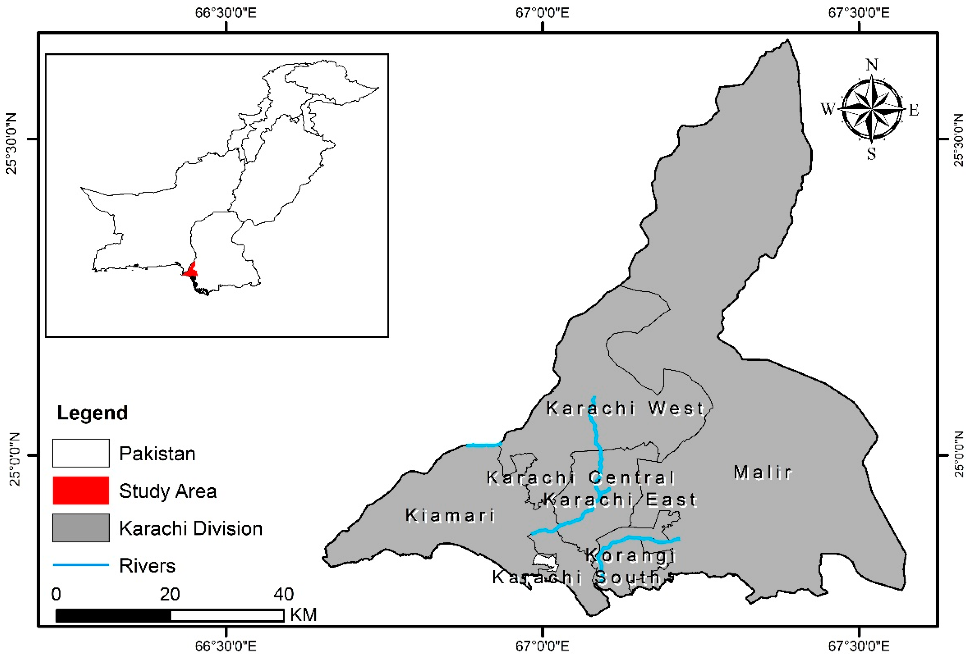
2.1. Study Area

Karachi, Pakistan’s largest and most densely populated city, is the provincial capital of Sindh Province. It is the country’s primary seaport, industrial center, and financial hub. The Karachi urban agglomeration, which covers 3527 km², is located on the Arabian Sea coastline between 24.45°N and 25.15°N and between 66.37°E and 67.37°E (Figure 1). The Lyari and Malir Rivers flow through the city on their way to the Arabian Sea. Administratively, the city is divided into seven districts and 31 subdivisions [34]. Karachi’s urban population has grown from 9.45 million in 1998 to 14.91 million in 2017. According to the United Nations’ estimates [35], the city’s population will reach more than 20 million by 2025. The rapid rate of urbanization during the last three decades has had negative consequences for the environment, specifically in relation to the UHI, air pollution, and energy consumption, as a result of the lack of urban expansion planning and insufficient essential public infrastructure and facilities [36].

2.2. Datasets

Eleven Landsat images acquired between 2000 and 2020 were utilized to map the land use/land cover changes and the urban thermal environment with 5-year intervals (Table 1). The images were acquired by Landsat 5 TM, 7 ETM+, and 8 OLI/TIRS. Landsat data consisted of collection 2, level 2 data obtained from the United States Geological Survey (https://earthexplorer.usgs.gov, accessed on 12 August 2021). The entire study area covered three Landsat tiles (152_042, 152_043, and 153_043). The land surface temperature could be determined from thermal infrared (TIR) measurements of satellite sensors. However, the TIR measurements are very sensitive to cloud contamination, which precludes an accurate determination of the LST [37]. In addition, precipitation can cause large variations in the surface emissivity. Thus, seasonal differences can influence remote sensing image availability (increased cloud cover) and accuracy in LST measurements. In order to reduce the uncertainties of LST determination, satellite images with a minimum amount of cloud coverage (<10%) corresponding to the driest months (September–November) were collected in our study [38,39]. Table 1 lists the ten Landsat scenes that were used for LST retrieval in this study.

3. Methods

In our study, the entire data processing and analysis workflow included several steps. First of all, the land use/land cover types were classified, and the land surface temperature was retrieved from the Landsat images. Thereafter, the intensity of the SUHI was quantified using the LST and land cover classification data. Finally, the relationship between the LST and land cover was explored. Figure 2 is an overview of the data processing workflow in this study.

3.1. Land Use/Land Cover Classification

The support vector machine (SVM) approach has been widely used for LULC classification with multisource remote sensing data and has exhibited its capacity to obtain accurate results [31,32,33]. The SVM classifier with a radial basis function kernel, and a penalty hyperparameter of 100 was used here to classify the land cover into four broad types: built-up area, bare land, water bodies, and vegetation. As one of the most widely used kernels, the radial basis function kernel is in the form of a Gaussian function and can obtain optimal results for nonlinear data. For each LULC class, around 150 samples were collected to ensure sufficient representation [40]. High-resolution satellite images in Google Earth and pan-sharpened versions of Landsat data were used to gather ground truth information [41]. The LULC classes and their descriptions are shown in Table 2, together with the number of training and testing pixels used during the SVM classification.
Quantitative metrics were used to assess the accuracy of each classified image. Ground truth regions for classification accuracy assessment were created using ancillary land cover change data from topographical maps and urban LULC maps acquired from the Survey department of Pakistan and Karachi Municipal Corporation [34]. The ground truth data were interpreted based on their spectral characteristics and a literature review with additional ancillary information.

3.2. Land Surface Temperature Retrieval

The land surface temperature was retrieved using a radiative transfer equation (RTE) [41]. Normalized LST values can provide objective information about the spatial distribution of the LST values extracted from satellite images obtained under a variety of atmospheric, temporal, and lighting conditions [42]. The LST values were standardized using Equation (1) to ensure the information extracted from satellite imagery captured over multiple years was comparable.
NLST = ( LST i LST min ) / ( LST max LST min ) ,
where NLST is the normalized LST, LST i is the pixel i initial LST, and LST min and LST max are the minimum and maximum LST in a given scene, respectively.

3.3. Calculation of the Surface Urban Heat Island Intensity

The most popular method for modeling the effects of urban growth and land cover change on the SUHII is to calculate the temperature differences between urban and rural areas. Since the definitions of urban and rural areas vary greatly from country to country, there is no standardized method to distinguish urban areas and rural areas [4]. Under the framework of the local climatic zone (LCZ), the SUHII was measured as the differential LST between built-up and green space areas [43]. As the LST within the areas of green space varied, an average LST was used as a reference for mapping SUHII. In this study, the SUHI intensity was measured as the difference in LSTs between built-up areas and areas of green space [44]. The SUHII was calculated for each built-up area pixel using Equation (2):
SUHII i = T b u i T ¯ g s ,
where T b u i is the land surface temperature at pixel i, and T ¯ g s , is the mean land surface temperature of the green space pixels. The green space pixels of the study area were determined using the LULC classification map. The SUHII for the whole study area was calculated using Equation (3):
SUHII = 1 n   i = 1 n SUHII i ,
where SUHII i is the surface urban heat island intensity at pixel i, and n is the total number of built-up pixels.
Following Reference [41], we classified the areas in the SUHII maps into five classes: no SUHII (SUHII < 0.00), low SUHII (0.00–2.00), moderate SUHII (2.00–4.00), high SUHII (4.00–6.00), and very high or extreme SUHII (>6.00).

3.4. Statistical Analysis

According to a systematic review [45], the majority of previous studies (>68%) tended to utilize global-based analysis to quantify the relationship between spatial variables and UHI variables. The ordinary least squares (OLS) regression, which assumes constant relationships over spaces between the independent and dependent variables, is the most commonly used approach. On the regional scale, however, the SUHI effect may be context-sensitive and vary considerably over time and location [46]. In this study, both bivariate correlation analysis and geographically weighted regression (GWR) were used to quantify the relationships between the LST and the land cover composition [47]. Pearson’s correlation coefficient was used to quantify the correlation between these two variables. We selected 1000 random samples to conduct a correlation analysis between the NLST, NDVI, and NDBI.
Geographically weighted regression is a technique in which the spatial heterogeneity of the relationships between the independent variables and the dependent variable can be captured [48,49]. The following formula was used for GWR:
y i = β 0 ( u i , v i ) + k β k ( u i , v i ) x i k + ε i ,
where ( u i , v i ) indicates the spatial coordinates of observation i, β 0 and β k are the estimated parameters, and ε i denotes the random error in terms of observation i. Each observation is assigned a weight based on the distance decay function. The weighting of an observation is not constant but is a function of the geographical location. Larger weights are assigned to observations closer to point i [50]. The inverse distance weighting has been adopted in different environmental studies [51,52,53]. In the GWR model, the relationships between the dependent and independent variables vary spatially [54]. The prediction performance of the GWR model can be improved by adjusting the regression coefficients according to the location. The kernel and bandwidth are the key parameters in the GWR model that affect the model accuracy. Herein, the adaptive Gaussian kernel was used because the 1000 sampling points were randomly distributed over an irregular study area. The model accuracy was evaluated using the coefficient of determination (R2) and corrected Akaike Information Criterion (AICc). In this research, the GWR models were developed using ArcGIS 10.5 software.

4. Results

4.1. Land Use/Land Cover Change Analysis

The overall accuracies of the land cover maps that were produced ranged from 86.2% to 94.28% (Table 3). Details of individual maps of land cover changes are shown in Table 3. The maps show a continued expansion in the built-up area of Karachi over the period 2000–2020 (Figure 3). In the center of the city, the percentage cover of the built-up area was highest in 2000. Since then, the built-up area has gradually extended outward into the suburbs. Moreover, the amount of open bare land decreased significantly. The result reveals an interesting two-stage pattern in the land cover changes, i.e., first, the open bare land and vegetation were converted to open land and then into built-up areas. Thus, areas that were open bare land and vegetation in 2000 were converted to open land by 2010 and to built-up areas by 2015. By 2020, these built-up areas had become denser.
Table 4 presents statistics for the LULC patterns in Karachi during the period 2000–2020. It can be seen that, between 2000 and 2020, the built-up area expanded by nearly 173%, from 440.19 km2 to 765.52 km2. Overall, the amount of vegetation cover and open bare land declined significantly over the same period. The amount of vegetation cover fluctuated, falling from 553.99 km2 to 428.07 km2 between 2000 and 2010 before increasing to 477.13 km2 in 2015 and, finally, declining again to 378.13 km2 in 2020. The amount of open bare land decreased from 2570.19 km2 in 2000 to 2390.58 km2 in 2020, whereas the area covered by water bodies increased from 43.54 km2 to 86.53 km2 between 2000 and 2020. A total of 179.61 km² of bare land and 175.86 km² of vegetation was converted into other land uses during this period (Figure 3). These LULC losses can be attributed to an increase in the urban area resulting from a high demand for residential space and space for business activities [55]. The open bare land and vegetation classes were those most affected by this rapid urbanization.
Figure 4 depicts the contribution of net changes in various LULC classes to changes in built-up areas. The Gadap, Bin Qasim, Murad Memon, Ibrahim Hyderi, Manghopir, Gulzar-i-Hijri Baldia, and Mauripur subdivisions experienced the largest increases in the built-up areas class. The smallest increases were in areas near the center of the city, such as The Garden, Saddar, Ferozabad, Harbor, Liaquatabad, SITE, Lyari, and Arambagh. Figure 4 shows that built-up area expansion primarily occurred due to the transformation of open bare land to built-up land in the northern and northeastern parts of the city. Vegetated areas were encroached upon by built-up areas in almost all parts of Karachi, except those near to the center. Moreover, in certain subdivisions, including The Garden, Saddar, Arambagh, Lyari, Civil Lines, Liaquatabad, and Harbor, there was only a slight increase in the area classed as built-up, because these were established CBD areas in which construction was restricted [56].

4.2. Spatiotemporal Variations in the Urban Thermal Environment

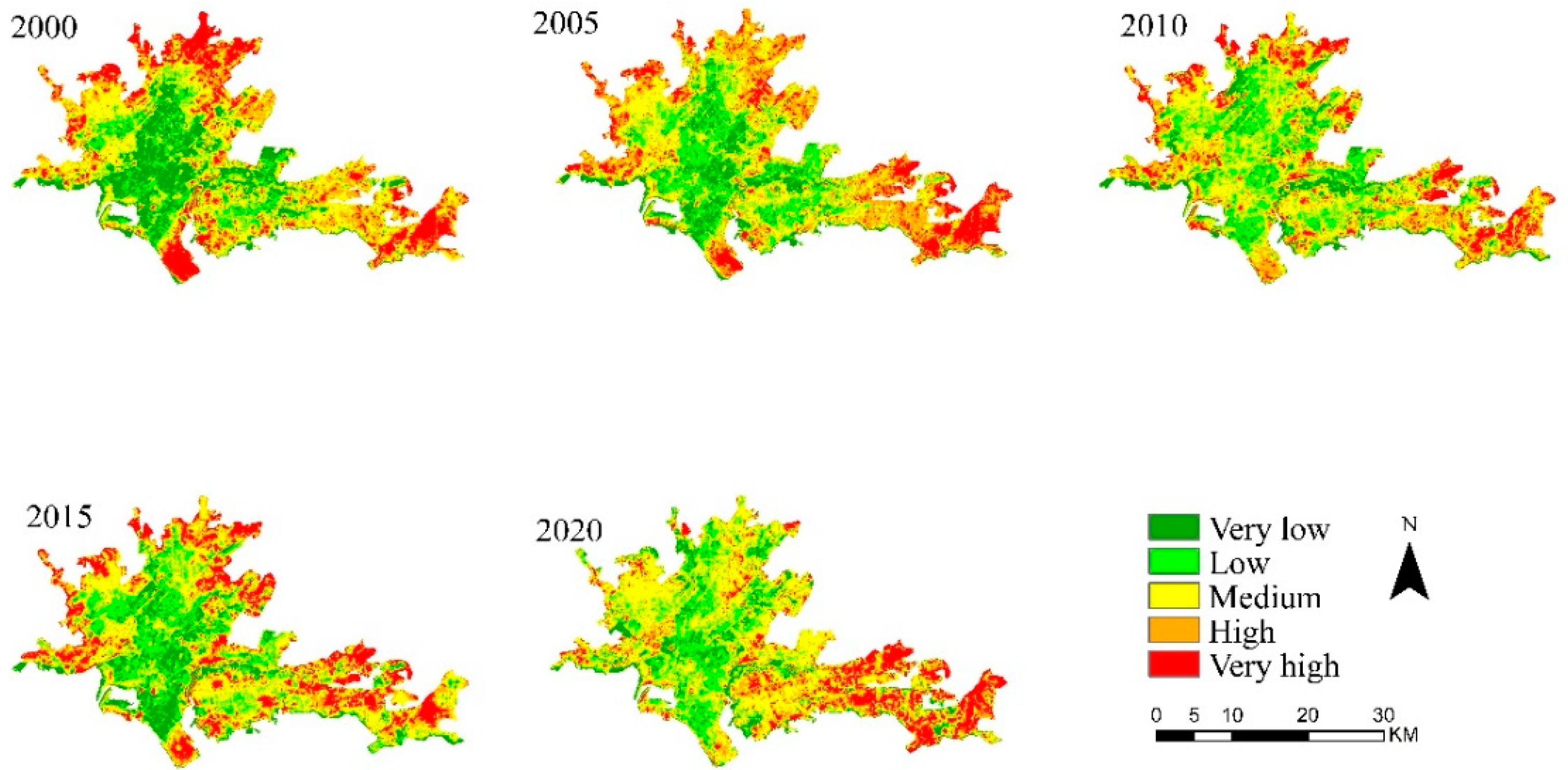
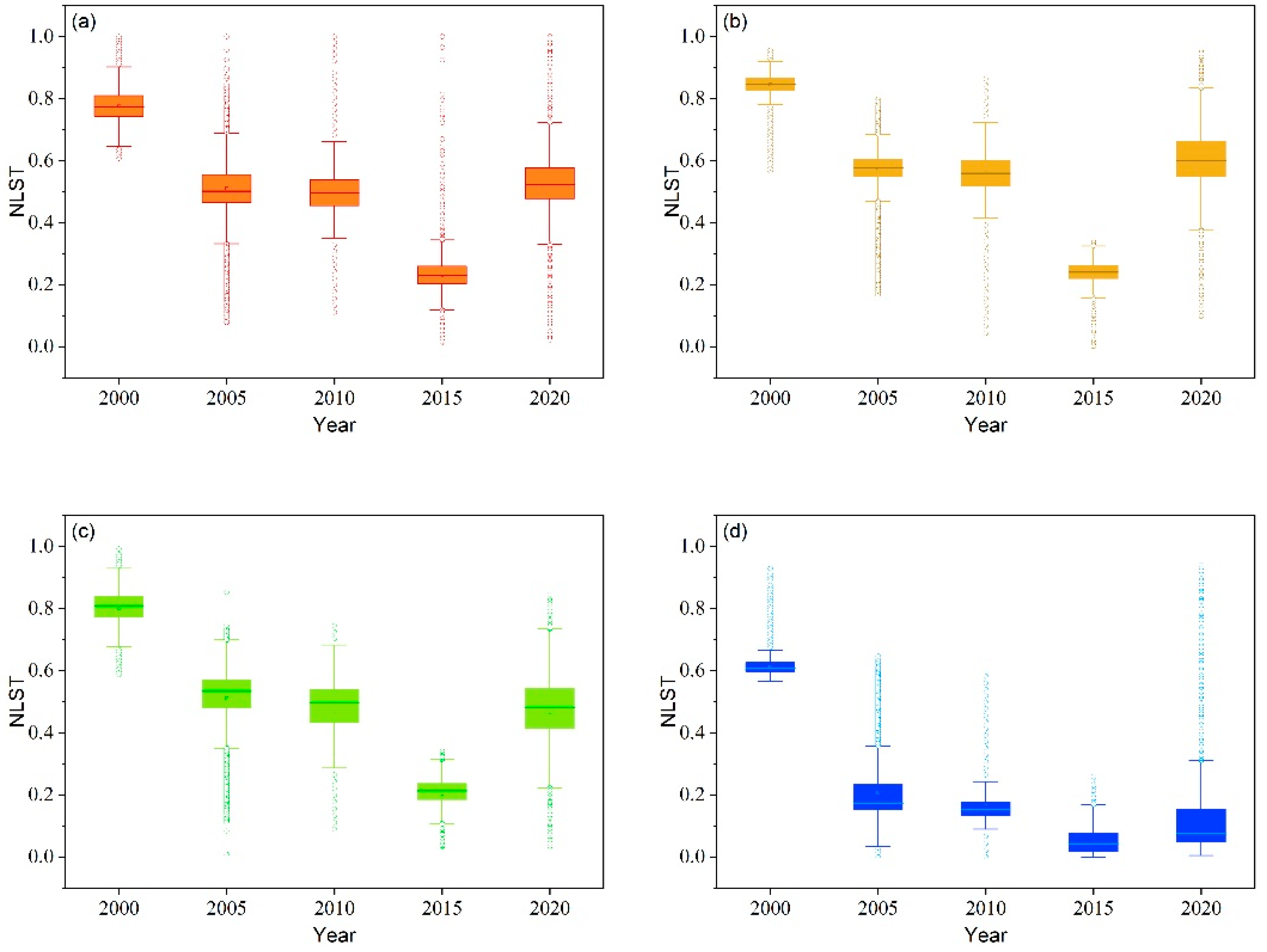
4.2.1. Variations in the Normalized Land Surface Temperature

Figure 5 shows the classified NLST maps of the study area. Each map shows five classes of NLST—namely, very low temperature, low temperature, medium temperature, high temperature, and very high temperature. They were defined using the standard deviation and mean value. Very high and high temperature areas were concentrated in the suburban areas, areas surrounding the suburbs, and in areas of open bare land; the main roads linking the city and the surrounding towns also appeared to have high or very high temperatures. Overall, the very high temperature class covered the majority of the suburbs. The area covered by each temperature class throughout the study period is shown in Table 5. The medium-temperature class covered the largest area over the five time periods, followed by the high-temperature class. Along with the decrease in the amount of green space, the area corresponding to the very low-temperature class also gradually decreased. In contrast, as a result of the built-up area expansion, the areas covered by the medium- and high-temperature classes increased considerably. The area of high and very high LST increased from 18,304.38 km2 in 2000 to 23,240.70 km2 in 2020 in the study area. Population growth, industrial development, the large number of vehicles, and traffic congestion are also connected to the increase in the areas denoted as being medium- and high-temperature classes [57,58].

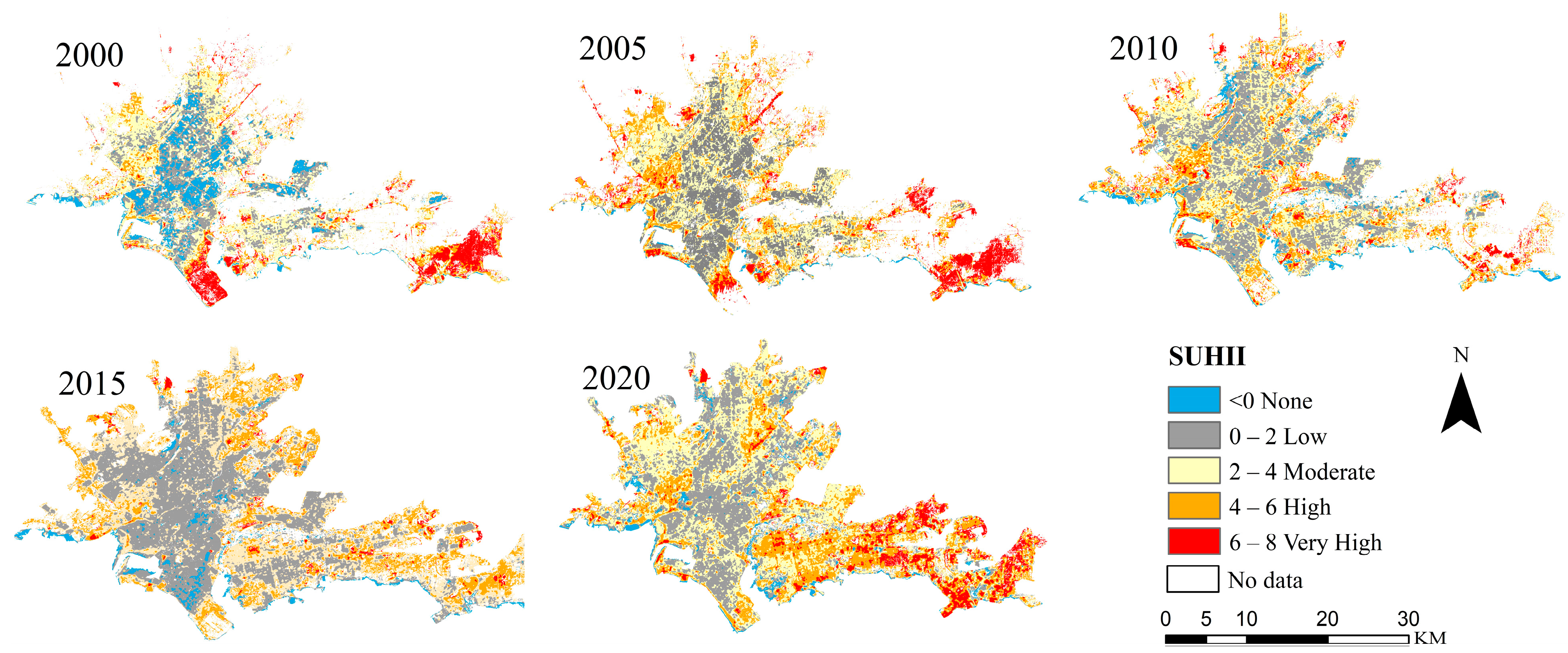
4.2.2. Variations in the Surface Urban Heat Island Intensity

The acquired satellite imagery was used to assess the spatiotemporal variations of SUHI over Karachi during the study period (2000–2020). The results showed that the SUHI intensity increased over this period due to the continual expansion of the built-up area. The areas corresponding to a very high, high, or moderate SUHII increased, whereas those in which the SUHII was classified as low or having no SUHI decreased to a certain extent (Table 6).
Figure 6 displays the spatial patterns of SUHII for different years during the study period. In 2000, the SUHII was very low in most of Karachi’s core areas; however, there were small pockets of moderate and high SUHII in the northwest, north, and south of the city. In the outskirts of Karachi, the situation was different. Very high SUHI zones increased from 0.21 hectares in 2000 to 0.33 hectares in 2020. Similarly, high and moderate zones increased from 0.29 and 0.55 hectares in 2000 to 0.95 and 01.39 hectares in 2020. These areas experienced haphazard expansion of the built-up areas during the study period and also included areas of exposed barren rocky outcrops that formed ridges and low hills. The exposed rocks with little vegetation coverage received direct solar radiation, which was converted into heat energy, resulting in a high LST. These factors resulted in a SUHI that was more intense than in the urban core [59].

4.3. Relationship between Variations of LST and Land Cover Changes

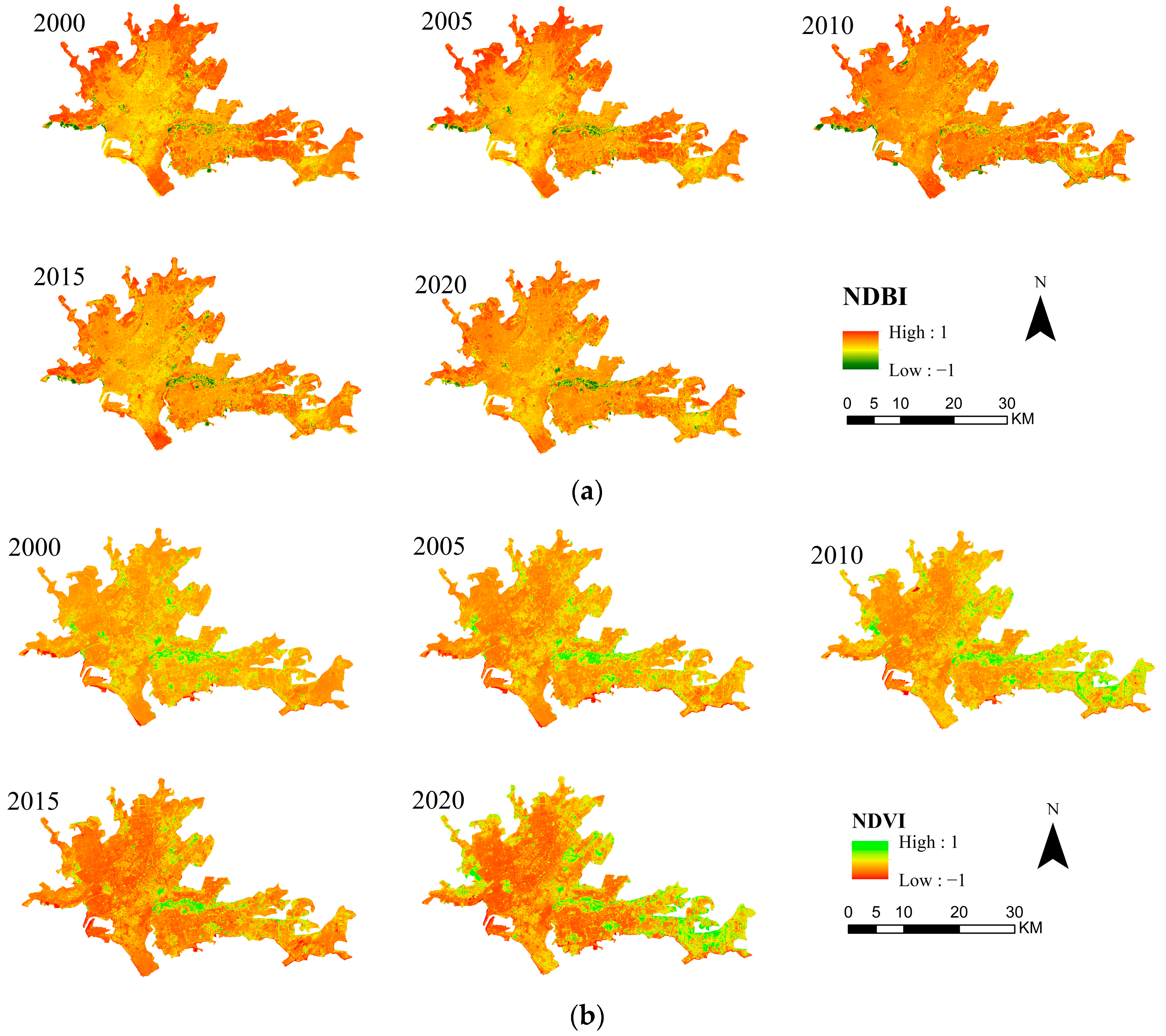
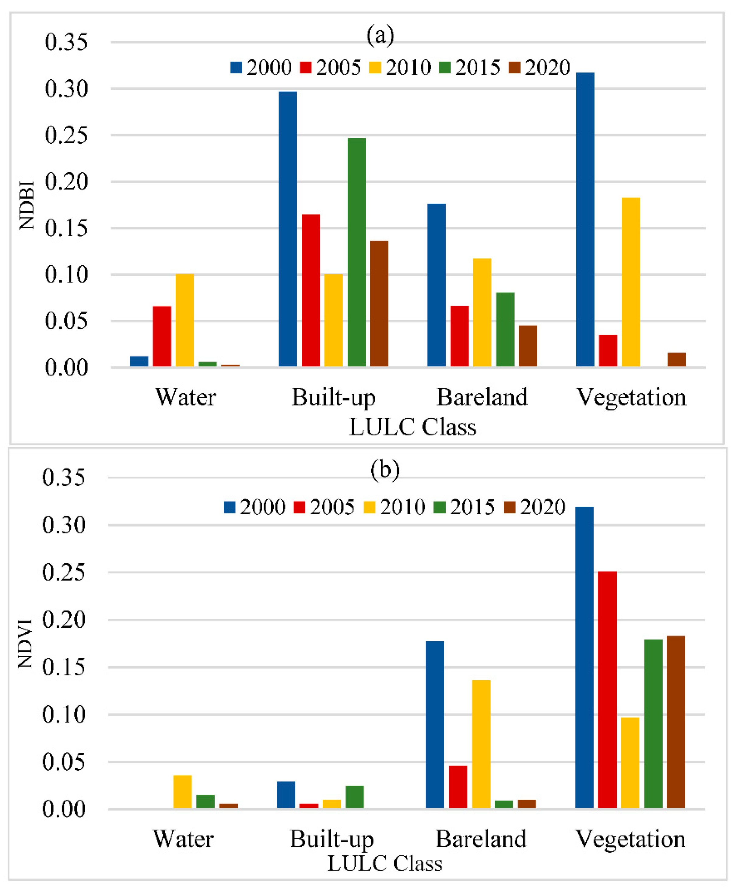
4.3.1. Relationship between Land Cover Types and Land Surface Temperature

The relationships between the NLST and the four land cover categories used in this study are illustrated in Figure 7. The increase in the NLST with time reflects the increase in the size and intensity of the urban heat island because of the land use/land cover changes and the built-up area expansion in the study area [41]. These trends have become more pronounced since 2000, as, after this date, the areas surrounding Karachi that were formerly agricultural and open bare land ceased to be cultivated and became built-up areas. Significant variations between the average NLST of the different land cover classes can be seen. For the vegetation and water body classes, a relatively large range of temperatures was observed over the study period. Changes in the vegetation density within the metropolitan area may be responsible for the LST variation for this class. Many investigators observed a negative relationship between the amount of vegetation and the land surface temperature [11,28]. As a result of the inclusion of mixed pixels, the land surface temperatures of the water bodies can be influenced by the temperature of the surroundings, for example, bare land. This may be a reason for the high NLST values observed in pixels that represent water bodies. It was observed that land cover types that were converted into built-up and open bare land classes were those for which the temperature increase was the greatest.

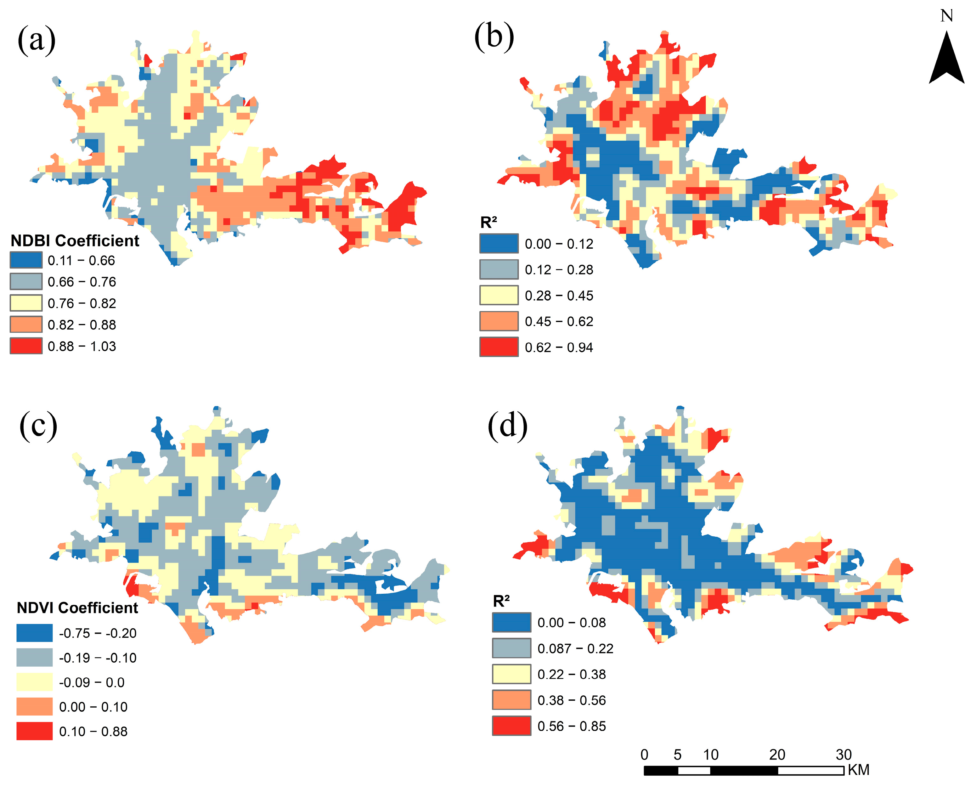
4.3.2. Relationship between Land Cover Composition and Normalized Land Surface Temperature

The NDVI and NDBI maps of Karachi for 2000 and 2020 are shown in Figure 8a,b, respectively. The NDVI values varied from −0.17 to 0.46 in 2000 and from −0.12 to 0.45 in 2020. In 2000 and 2020, high NDVI values were observed in the eastern part of the study area, which was covered by cultivated land. In 2000, the NDBI values were in the range of −0.40 to 0.36; in 2020, they were between −0.36 and 0.55. In 2000, areas with high NDBI values were mainly concentrated in the central and the northwest of the Malir River. By 2020, the area with high NDBI values had increased and also expanded to the southern and northeastern sides of the river (Figure 8b). These spatial patterns in the NDBI are consistent with the observed patterns in urban land use changes (Figure 3) and the NLST (Figure 6) in the study area.
The calculated Pearson’s correlation coefficient values indicated a significant positive correlation among the NLST and NDBI for all the land cover types throughout the study area (Figure 9). The built-up area exhibited the strongest correlation between the NDBI and NLST; the correlation was weakest for the areas covered by water bodies (0.012 in 2000 and 0.0026 in 2020). There was a weak correlation between the NLST with NDVI for all land cover types. This correlation was strongest for the vegetation class (0.319 in 2000 and 0.183 in 2020). The built-up and bare land categories exhibited the lowest correlation coefficients (0.029 and 0.177, respectively, in 2000 and 0.001 and 0.010, respectively, in 2020). The relationship between the NLST and NDVI demonstrated that the higher the vegetation density within a region, the lower the land surface temperature detected.
Figure 10 shows the distributions of the correlation coefficients for these two relationships, together with the corresponding values of the local adjusted R². The GWR analysis captured the spatial variation of the relationships between the NDVI and NDBI and the NLST. There was considerable spatial variation in the GWR results for different land cover classes. In the east and northeast of the study area, there was a strong positive correlation between the NLST and the NDBI, with coefficient values ranging from 0.82 to 0.88 in the urban core (Figure 10a). These areas mainly consisted of high-density urban residential and commercial areas and included the districts of Central, East, Korangi, and Kiamari. The CBD of Karachi is almost entirely built-up with sparsely distributed small-sized green spaces. The correlation between the NLST and the urban density was very low in these areas. The areas in which the correlation between the NLST and the NDVI was strongly negative were situated in the northern, eastern, and western parts of the study area (Figure 10c). These areas included large parks that have grasslands with dense vegetation. The relationship between the NDVI and NLST was very weak near to the coast. This may be due to the large uncertainty in the NDVI estimates that resulted from the presence of mixed pixels that included both water and vegetation. These uncertainties can be minimized by using remote sensing data from sensors with higher spatial resolution, such as Sentinel and Gaofen satellites [60,61,62]. Figure 10b, d demonstrate the GWR model’s overall fitness: a high adjusted R² value indicates good model fitness.

5. Discussion

In this study, we describe the rapid expansion in the built-up area of Karachi during the period from 2000 to 2020. It was shown that this expansion primarily occurred at the expense of areas that were previously planted with crops or were open bare land. Expansion of built-up areas at the expense of cropland during the process of urbanization has also been noted in other Pakistani metropolises, including Lahore [63], Peshawar [64], and Islamabad [65]. An important feature observed concerning LULC changes in Karachi during 2000–2020 was that the cropland and open bare land were first converted into areas of open land before becoming part of the built-up area. This type of change pattern was also observed in high-density metropolitan cities, such as Hyderabad [33] and Faisalabad [66]. This process was due to the fact that agricultural land and other types of land acquired by real estate companies were left open for many years before being rebuilt or restructured.
As compared to impervious surface types, such as roads, buildings, and industrial areas, the evapotranspiration in the vegetated areas is greater. In these areas, the vegetation canopy also provides shading, and as a result, the temperature is lower [67]. The rising trend in NLST across all land cover types implies an overall surface warming trend. Although the SUHII fluctuated, the proportion of areas in which the SUHII was classified as high increased in almost all subdistricts. The SUHII increased to the greatest extent in the subdivisions with the lowest vegetation cover. In these areas, shrubland and grassland were converted into high-density built-up areas. This is in accordance with the results of previous studies in which it was shown that the core areas of cities experience the greatest increase in SUHII due to the dense nature of the built-up area and the high population density [68]. In contrast, our study demonstrates that the SUHII increased more in the peripheral areas of Karachi, such as Korangi, Landhi, Ibrahim Hyderi, Bin Qasim, Shah Faisal, and Model Colony, than in the central areas. The greater rise in the SUHII in the countryside areas may be linked to the large-scale conversion of cropland and open bare land to built-up areas. The government encourages new housing schemes and the migration of people from central areas to suburban and rural areas. The new housing schemes increase the funding of public infrastructures, educational institutes, and transportation networks to CBD areas. However, the SUHII in these areas is exacerbated by the rapid construction of the new settlements and other public infrastructures.
The regression analysis results presented in this study suggest that the GWR model can produce good results and provide detailed information at the local scale. According to the adjusted R² values, the GWR model can explain 84% of the variation in the land surface temperature in the study area [69,70]. From north to south, there was a trend from a negative correlation to a positive NDVI correlation, with the values of the adjusted NDVI R² ranging from −3.159 to 4.195. According to the land cover classification results, the built-up area density in the southern part of the city core was low. To the north of the core area, the vegetation density was high and stable, and the variations of the NDVI were observed to have a significant impact on the LST. This can be attributed to the strong cooling effect that vegetation produces in these areas. This study found that aggregated green space in parks was more effective in terms of providing cooling effects than scattered vegetation patches in the urban core. Increasing the total area and aggregation level of green space can considerably alleviate the negative impact of urban heat islands. Furthermore, in Pakistan, geospatial data are not freely shared due to various institutional and technical problems [71,72]. The openness of geospatial data collected by different government departments can facilitate the understanding of the relationship between urbanization and UHI.
Although this study provides a comprehensive description of SUHI variability, further work is necessary to investigate the influence of the spatial patterns in LULC on the SUHII, as this remains unclear. This can be achieved by applying high-resolution remote sensing data and multiscale landscape pattern analysis approaches [41,73]. Moreover, a time series analysis could provide a more precise picture of the SUHI variation in Karachi in relation to LULC changes. The findings of this study are restricted to one coastal city in Pakistan. The association between LST and land cover may vary in different cities. Therefore, to fully grasp the impacts of urban land cover characteristics on the LST, the relationship between LULC and the LST should be examined by comparing cities in different settings [74].

6. Conclusions

The analysis of LULC change and its influence on the SUHII and the urban thermal environment of Karachi performed in this study demonstrated that the SUHII grew exponentially in Karachi during the period from 2000 to 2020. The size of the built-up area increased massively, whereas the amount of open bare land declined by more than 76.76% during this period, and the area covered by vegetation increased by 68.35%. These changes significantly altered the patterns of SUHII within Karachi, Pakistan. During the study period, the areas in which the SUHII intensity was classified as moderate, high, and very high increased from 0.55% to 1.39%, 0.29% to 0.96%, and 0.21% to 0.33% of the study area, respectively. It was also found that the SUHII increased to the greatest extent in the peripheral subdivisions in the eastern and northern parts of the city, in which there was the greatest expansion in the urban area at the expense of areas of vegetation and open bare land.
The GWR technique was used in this study. The highest NDBI regression coefficients were found in the districts situated in the east and the west, including Kamari and Malir. The southern and central parts of the city were found to have the lowest NDBI coefficients. This information could aid decision-makers in developing policies at the regional scale and fine-tuning planning practices at the local scale, with the aim of improving thermal conditions and promoting sustainable development in less-developed regions. From the regression coefficient map, the areas in which green space was most effective in terms of mitigating UHI effects were identified. Large- and medium-sized parks with dense and aggregated vegetation coverage are recommended in order to improve the thermal environment in Karachi. Moreover, future land use and land cover changes can be modeled to help decision-makers enhance the thermal resilience in cities under different land change conditions more effectively.

Author Contributions

Conceptualization, L.L. and F.C.; methodology, M.F.B., L.P. and S.N.-u.-H.; formal analysis, M.F.B., L.P. and B.L.; writing—original draft preparation, L.L. and M.F.B.; writing—review and editing, L.L., M.F.B., F.C., S.Q., S.N.-u.-H., A.T. and Q.L.; and funding acquisition, L.L. All authors have read and agreed to the published version of the manuscript.

Funding

This work was supported by the Strategic Priority Research Program of the Chinese Academy of Sciences (grant number XDA19030502) and the National Natural Science Foundation of China (grant number 42071321).

Data Availability Statement

The data presented in this study are available on request from the corresponding author.

Acknowledgments

The authors are grateful for the comments from the anonymous reviewers and the editors.

Conflicts of Interest

The authors declare no conflict of interest.

References

  1. Angel, S.; Parent, J.; Civco, D.L.; Blei, A.; Potere, D. The dimensions of global urban expansion: Estimates and projections for all countries, 2000–2050. Prog. Plan. 2011, 75, 53–107. [Google Scholar] [CrossRef]
  2. Department of Economic and Social Affairs. World Urbanization Prospects: The 2018 Revision; Department of Economic and Social Affairs, UN: New York, NY, USA, 2019. [Google Scholar]
  3. Zhou, M.; Lu, L.; Guo, H.; Weng, Q.; Cao, S.; Zhang, S.; Li, Q. Urban Sprawl and Changes in Land-Use Efficiency in the Beijing–Tianjin–Hebei Region, China from 2000 to 2020: A Spatiotemporal Analysis Using Earth Observation Data. Remote Sens. 2021, 13, 2850. [Google Scholar] [CrossRef]
  4. Oke, T.R.; Stewart, I.D. Local Climate Zones for Urban Temperature Studies. Bull. Am. Meteorol. Soc. 2012, 93, 1879–1900. [Google Scholar] [CrossRef]
  5. Lu, L.; Weng, Q.; Guo, H.; Feng, S.; Li, Q. Assessment of urban environmental change using multi-source remote sensing time series (2000–2016): A comparative analysis in selected megacities in Eurasia. Sci. Total Environ. 2019, 684, 567–577. [Google Scholar] [CrossRef]
  6. Sobrino, J.A.; Oltra-Carrió, R.; Sòria, G.; Jiménez-Muñoz, J.C.; Franch, B.; Hidalgo, V.; Mattar, C.; Julien, Y.; Cuenca, J.; Romaguera, M.; et al. Evaluation of the surface urban heat island effect in the city of Madrid by thermal remote sensing. Int. J. Remote Sens. 2013, 34, 3177–3192. [Google Scholar] [CrossRef]
  7. Grimmond, S. Urbanization and Global Environmental Change: Local Effects of Urban Warming. Geogr. J. 2007, 173, 83–88. Available online: https://www.jstor.org/stable/30113496 (accessed on 15 July 2021). [CrossRef]
  8. Kikegawa, Y.; Genchi, Y.; Yoshikado, H.; Kondo, H. Development of a numerical simulation system toward comprehensive assessments of urban warming countermeasures including their impacts upon the urban buildings’ energy-demands. Appl. Energy 2003, 76, 449–466. [Google Scholar] [CrossRef]
  9. Lu, L.; Guo, H.; Corbane, C.; Li, Q. Urban sprawl in provincial capital cities in China: Evidence from multi-temporal urban land products using Landsat data. Sci. Bull. 2019, 64, 955–957. [Google Scholar] [CrossRef] [Green Version]
  10. Güneralp, B.; Lwasa, S.; Masundire, H.; Parnell, S.; Seto, K.C. Urbanization in Africa: Challenges and opportunities for conservation. Environ. Res. Lett. 2017, 13, 015002. [Google Scholar] [CrossRef]
  11. Hassan, T.; Zhang, J.; Prodhan, F.A.; Pangali Sharma, T.P.; Bashir, B. Surface Urban Heat Islands Dynamics in Response to LULC and Vegetation across South Asia (2000–2019). Remote Sens. 2021, 13, 3177. [Google Scholar] [CrossRef]
  12. Kikon, N.; Singh, P.; Singh, S.K.; Vyas, A. Assessment of urban heat islands (UHI) of Noida City, India using multi-temporal satellite data. Sustain. Cities Soc. 2016, 22, 19–28. [Google Scholar] [CrossRef]
  13. Arshad, S.; Ahmad, S.R.; Abbas, S.; Asharf, A.; Siddiqui, N.A.; Islam, Z.U. Quantifying the contribution of diminishing green spaces and urban sprawl to urban heat island effect in a rapidly urbanizing metropolitan city of Pakistan. Land Use Policy 2022, 113, 105874. [Google Scholar] [CrossRef]
  14. Waseem, S.; Khayyam, U. Loss of vegetative cover and increased land surface temperature: A case study of Islamabad, Pakistan. J. Clean. Prod. 2019, 234, 972–983. [Google Scholar] [CrossRef]
  15. Cai, D.; Fraedrich, K.; Guan, Y.; Guo, S.; Zhang, C. Urbanization and the thermal environment of Chinese and US-American cities. Sci. Total Environ. 2017, 589, 200–211. [Google Scholar] [CrossRef] [Green Version]
  16. Peng, J.; Jia, J.; Liu, Y.; Li, H.; Wu, J. Seasonal contrast of the dominant factors for spatial distribution of land surface temperature in urban areas. Remote Sens. Environ. 2018, 215, 255–267. [Google Scholar] [CrossRef]
  17. Li, J.; Song, C.; Cao, L.; Zhu, F.; Meng, X.; Wu, J. Impacts of landscape structure on surface urban heat islands: A case study of Shanghai, China. Remote Sens. Environ. 2011, 115, 3249–3263. [Google Scholar] [CrossRef]
  18. Liu, L.; Zhang, Y. Urban heat island analysis using the Landsat TM data and ASTER data: A case study in Hong Kong. Remote Sens. 2011, 3, 1535–1552. [Google Scholar] [CrossRef] [Green Version]
  19. Zhou, D.; Bonafoni, S.; Zhang, L.; Wang, R. Remote sensing of the urban heat island effect in a highly populated urban agglomeration area in East China. Sci. Total Environ. 2018, 628, 415–429. [Google Scholar] [CrossRef]
  20. Choi, Y.-Y.; Suh, M.-S.; Park, K.-H. Assessment of surface urban heat islands over three megacities in East Asia using land surface temperature data retrieved from COMS. Remote Sens. 2014, 6, 5852–5867. [Google Scholar] [CrossRef] [Green Version]
  21. Maharjan, M.; Aryal, A.; Man Shakya, B.; Talchabhadel, R.; Thapa, B.R.; Kumar, S. Evaluation of Urban Heat Island (UHI) Using Satellite Images in Densely Populated Cities of South Asia. Earth 2021, 2, 86–110. [Google Scholar] [CrossRef]
  22. Tran, H.; Uchihama, D.; Ochi, S.; Yasuoka, Y. Assessment with satellite data of the urban heat island effects in Asian mega cities. Int. J. Appl. Earth Obs. Geoinf. 2006, 8, 34–48. [Google Scholar] [CrossRef]
  23. Lee, K.; Kim, Y.; Sung, H.C.; Ryu, J.; Jeon, S.W. Trend analysis of urban heat island intensity according to urban area change in Asian mega cities. Sustainability 2020, 12, 112. [Google Scholar] [CrossRef] [Green Version]
  24. Petropoulos, G.; Ireland, G.; Griffiths, H.; Islam, T.; Kalivas, D.; Anagnostopoulos, V.; Hodges, C.; Srivastava, P. Spatiotemporal estimates of surface Soil Moisture from space using the Ts/VI feature space. In Satellite Soil Moisture Retrieval; Elsevier: Amsterdam, The Netherlands, 2016; pp. 91–108. [Google Scholar]
  25. Guha, S.; Govil, H.; Dey, A.; Gill, N. Analytical study of land surface temperature with NDVI and NDBI using Landsat 8 OLI and TIRS data in Florence and Naples city, Italy. Eur. J. Remote Sens. 2018, 51, 667–678. [Google Scholar] [CrossRef]
  26. Chen, X.-L.; Zhao, H.-M.; Li, P.-X.; Yin, Z.-Y. Remote sensing image-based analysis of the relationship between urban heat island and land use/cover changes. Remote Sens. Environ. 2006, 104, 133–146. [Google Scholar] [CrossRef]
  27. Zhou, G.; Wang, H.; Chen, W.; Zhang, G.; Luo, Q.; Jia, B. Impacts of Urban land surface temperature on tract landscape pattern, physical and social variables. Int. J. Remote Sens. 2020, 41, 683–703. [Google Scholar] [CrossRef]
  28. Rizvi, S.H.; Fatima, H.; Iqbal, M.J.; Alam, K. The effect of urbanization on the intensification of SUHIs: Analysis by LULC on Karachi. J. Atmos. Sol.-Terr. Phys. 2020, 207, 105374. [Google Scholar] [CrossRef]
  29. Ranagalage, M.; Morimoto, T.; Simwanda, M.; Murayama, Y. Spatial analysis of urbanization patterns in four rapidly growing south Asian cities using Sentinel-2 Data. Remote Sens. 2021, 13, 1531. [Google Scholar] [CrossRef]
  30. Salim, A.; Ahmed, A.; Ashraf, N.; Ashar, M. Deadly Heat Wave in Karachi, July 2015: Negligence or Mismanagement? Int. J. Occup. Environ. Med. 2015, 6, 249. [Google Scholar] [CrossRef] [Green Version]
  31. Rahman, A.; Abdullah, H.M.; Tanzir, M.T.; Hossain, M.J.; Khan, B.M.; Miah, M.G.; Islam, I. Performance of different machine learning algorithms on satellite image classification in rural and urban setup. Remote Sens. Appl. Soc. Environ. 2020, 20, 100410. [Google Scholar] [CrossRef]
  32. Hassan, Z.; Shabbir, R.; Ahmad, S.S.; Malik, A.H.; Aziz, N.; Butt, A.; Erum, S. Dynamics of land use and land cover change (LULCC) using geospatial techniques: A case study of Islamabad Pakistan. SpringerPlus 2016, 5, 812. [Google Scholar] [CrossRef] [Green Version]
  33. Ul Din, S.; Mak, H.W.L. Retrieval of Land-Use/Land Cover Change (LUCC) Maps and Urban Expansion Dynamics of Hyderabad, Pakistan via Landsat Datasets and Support Vector Machine Framework. Remote Sens. 2021, 13, 3337. [Google Scholar] [CrossRef]
  34. Pakistan Bureau of Statistics. Government of Pakistan. 2017. Available online: https://www.pbs.gov.pk/content/final-results-census-2017 (accessed on 31 July 2021).
  35. Bremner, J.; Frost, A.; Haub, C.; Mather, M.; Ringheim, K.; Zuehlke, E. World population highlights: Key findings from PRB’s 2010 world population data sheet. Popul. Bull. 2010, 65, 1–12. [Google Scholar]
  36. Baqa, M.F.; Chen, F.; Lu, L.; Qureshi, S.; Tariq, A.; Wang, S.; Jing, L.; Hamza, S.; Li, Q. Monitoring and Modeling the Patterns and Trends of Urban Growth Using Urban Sprawl Matrix and CA-Markov Model: A Case Study of Karachi, Pakistan. Land 2021, 10, 700. [Google Scholar] [CrossRef]
  37. Neteler, M. Estimating daily land surface temperatures in mountainous environments by reconstructed MODIS LST data. Remote Sens. 2010, 2, 333–351. [Google Scholar] [CrossRef] [Green Version]
  38. Shaikh, A.A.; Gotoh, K. A satellite remote sensing evaluation of urban land cover changes and its associated impacts on water resources in Karachi, Pakistan. NED Univ. J. Res. 2008, 5, 41–56. [Google Scholar] [CrossRef]
  39. Tomlinson, C.J.; Chapman, L.; Thornes, J.E.; Baker, C. Remote sensing land surface temperature for meteorology and climatology: A review. Meteorol. Appl. 2011, 18, 296–306. [Google Scholar] [CrossRef] [Green Version]
  40. Shih, H.-c.; Stow, D.A.; Tsai, Y.H. Guidance on and comparison of machine learning classifiers for Landsat-based land cover and land use mapping. Int. J. Remote Sens. 2019, 40, 1248–1274. [Google Scholar] [CrossRef]
  41. Lu, L.; Weng, Q.; Xiao, D.; Guo, H.; Li, Q.; Hui, W. Spatiotemporal Variation of Surface Urban Heat Islands in Relation to Land Cover Composition and Configuration: A Multi-Scale Case Study of Xi’an, China. Remote Sens. 2020, 12, 2713. [Google Scholar] [CrossRef]
  42. Firozjaei, M.K.; Kiavarz, M.; Alavipanah, S.K.; Lakes, T.; Qureshi, S. Monitoring and forecasting heat island intensity through multi-temporal image analysis and cellular automata-Markov chain modelling: A case of Babol city, Iran. Ecol. Indic. 2018, 91, 155–170. [Google Scholar] [CrossRef]
  43. Bechtel, B.; Demuzere, M.; Mills, G.; Zhan, W.; Sismanidis, P.; Small, C.; Voogt, J. SUHI analysis using Local Climate Zones—A comparison of 50 cities. Urban Clim. 2019, 28, 100451. [Google Scholar] [CrossRef]
  44. Estoque, R.C.; Murayama, Y. Monitoring surface urban heat island formation in a tropical mountain city using Landsat data (1987–2015). ISPRS J. Photogramm. Remote Sens. 2017, 133, 18–29. [Google Scholar] [CrossRef]
  45. Deilami, K.; Kamruzzaman, M.; Liu, Y. Urban heat island effect: A systematic review of spatio-temporal factors, data, methods, and mitigation measures. Int. J. Appl. Earth Obs. Geoinf. 2018, 67, 30–42. [Google Scholar] [CrossRef]
  46. Buyantuyev, A.; Wu, J. Urban heat islands and landscape heterogeneity: Linking spatiotemporal variations in surface temperatures to land-cover and socioeconomic patterns. Landsc. Ecol. 2010, 25, 17–33. [Google Scholar] [CrossRef]
  47. Siqi, J.; Yuhong, W. Effects of land use and land cover pattern on urban temperature variations: A case study in Hong Kong. Urban Clim. 2020, 34, 100693. [Google Scholar] [CrossRef]
  48. Chen, T.-L.; Lin, Z.-H. Impact of land use types on the spatial heterogeneity of extreme heat environments in a metropolitan area. Sustain. Cities Soc. 2021, 72, 103005. [Google Scholar] [CrossRef]
  49. Hamza, S.; Khan, I.; Lu, L.; Liu, H.; Burke, F.; Nawaz-ul-Huda, S.; Baqa, M.F.; Tariq, A. The Relationship between Neighborhood Characteristics and Homicide in Karachi, Pakistan. Sustainability 2021, 13, 5520. [Google Scholar] [CrossRef]
  50. Yang, W. An Extension of Geographically Weighted Regression with Flexible Bandwidths. Ph.D. Thesis, University of St Andrews, St Andrews, UK, 2014. [Google Scholar]
  51. Arif, M.; Hussain, I.; Hussain, J.; Sharma, M.K.; Kumar, S.; Bhati, G. GIS-based inverse distance weighting spatial interpolation technique for fluoride distribution in south west part of Nagaur district, Rajasthan. Cogent Environ. Sci. 2015, 1, 1038944. [Google Scholar] [CrossRef]
  52. Mak, H.W.; Ng, D.C. Spatial and Socio-Classification of Traffic Pollutant Emissions and Associated Mortality Rates in High-Density Hong Kong via Improved Data Analytic Approaches. Int. J. Environ. Res. Public Health 2021, 18, 6532. [Google Scholar] [CrossRef]
  53. Ke, W.; Cheng, H.P.; Yan, D.; Lin, C. The Application of Cluster Analysis and Inverse Distance-Weighted Interpolation to Appraising the Water Quality of Three Forks Lake. Procedia Environ. Sci. 2011, 10, 2511–2517. [Google Scholar] [CrossRef] [Green Version]
  54. Szymanowski, M.; Kryza, M. Local regression models for spatial interpolation of urban heat island—an example from Wrocław, SW Poland. Theor. Appl. Climatol. 2012, 108, 53–71. [Google Scholar] [CrossRef] [Green Version]
  55. Hasan, A. Land contestation in Karachi and the impact on housing and urban development. Environ. Urban. 2015, 27, 217–230. [Google Scholar] [CrossRef] [PubMed] [Green Version]
  56. Building, K.; Regulations, T.P. Chapter 25. Historic Buildings. Sindh Building Control. In Authority (SBCA) Department of Culture and Planning; Government of Pakistan: Islamabad, Pakistan, 2002. [Google Scholar]
  57. Mehdi, M.R.; Kim, M.; Seong, J.C.; Arsalan, M.H. Spatio-temporal patterns of road traffic noise pollution in Karachi, Pakistan. Environ. Int. 2011, 37, 97–104. [Google Scholar] [CrossRef] [PubMed]
  58. Qureshi, S. The fast growing megacity Karachi as a frontier of environmental challenges: Urbanization and contemporary urbanism issues. J. Geogr. Reg. Plan. 2010, 3, 306–321. [Google Scholar] [CrossRef]
  59. Pithawalla, M.B.; Martin-Kaye, P.H.A. Geology and geography of Karachi and its neighbourhood; University Microfilms: Ann Arbor, MI, USA, 1962. [Google Scholar]
  60. Van Leeuwen, W.J.; Orr, B.J.; Marsh, S.E.; Herrmann, S.M. Multi-sensor NDVI data continuity: Uncertainties and implications for vegetation monitoring applications. Remote Sens. Environ. 2006, 100, 67–81. [Google Scholar] [CrossRef]
  61. Roy, D.P.; Borak, J.S.; Devadiga, S.; Wolfe, R.E.; Zheng, M.; Descloitres, J. The MODIS Land product quality assessment approach. Remote Sens. Environ. 2002, 83, 62–76. [Google Scholar] [CrossRef]
  62. Ghimire, P.; Lei, D.; Juan, N. Effect of image fusion on vegetation index quality—a comparative study from Gaofen-1, Gaofen-2, Gaofen-4, Landsat-8 OLI and MODIS Imagery. Remote Sens. 2020, 12, 1550. [Google Scholar] [CrossRef]
  63. Mumtaz, F.; Tao, Y.; de Leeuw, G.; Zhao, L.; Fan, C.; Elnashar, A.; Bashir, B.; Wang, G.; Li, L.; Naeem, S.; et al. Modeling Spatio-Temporal Land Transformation and Its Associated Impacts on land Surface Temperature (LST). Remote Sens. 2020, 12, 2987. [Google Scholar] [CrossRef]
  64. Ahmad, W.; Iqbal, J.; Nasir, M.J.; Ahmad, B.; Khan, M.T.; Khan, S.N.; Adnan, S. Impact of land use/land cover changes on water quality and human health in district Peshawar Pakistan. Sci. Rep. 2021, 11, 16526. [Google Scholar] [CrossRef]
  65. Sadiq Khan, M.; Ullah, S.; Sun, T.; Rehman, A.U.; Chen, L. Land-Use/Land-Cover Changes and Its Contribution to Urban Heat Island: A Case Study of Islamabad, Pakistan. Sustainability 2020, 12, 3861. [Google Scholar] [CrossRef]
  66. Dilawar, A.; Chen, B.; Trisurat, Y.; Tuankrua, V.; Arshad, A.; Hussain, Y.; Measho, S.; Guo, L.; Kayiranga, A.; Zhang, H.; et al. Spatiotemporal shifts in thermal climate in responses to urban cover changes: A-case analysis of major cities in Punjab, Pakistan. Geomat. Nat. Hazards Risk 2021, 12, 763–793. [Google Scholar] [CrossRef]
  67. Bowler, D.E.; Buyung-Ali, L.; Knight, T.M.; Pullin, A.S. Urban greening to cool towns and cities: A systematic review of the empirical evidence. Landsc. Urban. Plan. 2010, 97, 147–155. [Google Scholar] [CrossRef]
  68. Atasoy, M. Assessing the impacts of land-use/land-cover change on the development of urban heat island effects. Environ. Dev. Sustain. 2020, 22, 7547–7557. [Google Scholar] [CrossRef]
  69. Alibakhshi, Z.; Ahmadi, M.; Farajzadeh Asl, M. Modeling biophysical variables and land surface temperature using the GWR model: Case study—Tehran and its satellite cities. J. Indian Soc. Remote Sens. 2020, 48, 59–70. [Google Scholar] [CrossRef]
  70. Kashki, A.; Karami, M.; Zandi, R.; Roki, Z. Evaluation of the effect of geographical parameters on the formation of the land surface temperature by applying OLS and GWR, A case study Shiraz City, Iran. Urban Clim. 2021, 37, 100832. [Google Scholar] [CrossRef]
  71. Khurshid, M.M.; Zakaria, N.; Rashid, A.; Kazmi, R.; Shafique, M. Diffusion of Big Open Data Policy Innovation in Government and Public Bodies in Pakistan. In Proceedings of the First International Conference, INTAP 2018, Bahawalpur, Pakistan, 23–25 October 2018; Revised Selected Papers. Springer: Berlin/Heidelberg, Germany, 2019; pp. 326–337. [Google Scholar] [CrossRef]
  72. Khurshid, M.M.; Zakaria, N.; Rashid, A.; Ahmad, M.; Arfeen, M.; Faisal, H. Modeling of Open Government Data for Public Sector Organizations Using the Potential Theories and Determinants—A Systematic Review. Informatics 2020, 7, 24. [Google Scholar] [CrossRef]
  73. Peng, J.; Hu, Y.; Dong, J.; Liu, Q.; Liu, Y. Quantifying spatial morphology and connectivity of urban heat islands in a megacity: A radius approach. Sci. Total Environ. 2020, 714, 136792. [Google Scholar] [CrossRef] [PubMed]
  74. Koc, C.B.; Osmond, P.; Peters, A. Evaluating the cooling effects of green infrastructure: A systematic review of methods, indicators and data sources. Sol. Energy 2018, 166, 486–508. [Google Scholar] [CrossRef]
Figure 1. The geographical location of the study area.
Remotesensing 14 02164 g001
Figure 2. Data processing workflow.
Remotesensing 14 02164 g002
Figure 3. LULC maps of the study area estimated from Landsat data for the years 2000, 2005, 2010, 2015, and 2020.
Remotesensing 14 02164 g003
Figure 4. Details of the transition from other land use/land cover types to the built-up area class: (A) 2000–2010 and (B) 2010–2020.
Remotesensing 14 02164 g004
Figure 5. NLST classification map in 2000, 2005, 2010, 2015, and 2020.
Remotesensing 14 02164 g005
Figure 6. Spatial patterns in the SUHII (°C) in the study area for five different years during the period 2000–2020.
Remotesensing 14 02164 g006
Figure 7. Box plots of normalized land surface temperatures for different land cover types: (a) built-up area, (b) bare land, (c) vegetation, and (d) water bodies.
Remotesensing 14 02164 g007
Figure 8. Maps of the (a) NDBI and (b) NDVI for Karachi for 2000, 2005, 2010, 2015, and 2020.
Remotesensing 14 02164 g008
Figure 9. Relationship between the NLST and (a) NDVI and (b) NDBI, as given by the Pearson’s correlation coefficient value.
Remotesensing 14 02164 g009
Figure 10. Results of the GWR analysis: correlation coefficients between the NLST and (a) the NDBI and (b) the corresponding local R2 and correlation coefficients between the NLST and (c) the NDVI and (d) the corresponding local R2.
Remotesensing 14 02164 g010
Table 1. Details of the Landsat imagery used.
YearDateSatellite and SensorSpatial Resolution (m)
200026 October 2000Landsat5 TM30
1 October 2000Landsat5 TM30
200516 October 2005Landsat7 ETM+30
7 October 2006Landsat5 TM30
20107 November 2010Landsat5 TM30
21 October 2010Landsat7 ETM+30
20155 November 2015Landsat8 OLI30
12 November 2015Landsat8 OLI30
20201 October 2020Landsat8 OLI30
24 October 2020Landsat8 OLI30
Table 2. LULC classification scheme and class descriptions.
LULC ClassDescriptionNo. of Training PixelsNo. of Testing Pixels
Water bodiesRivers, permanent open water, lakes, ponds, and reservoirs60120
Built-up areaResidential areas, land used for commerce and services, industry, transportation, and roads150240
VegetationAgricultural areas, crops, fallow land and vegetation, and scrub150240
Bare landExposed soils, landfill sites, areas of active excavation, and open bare land150240
Table 3. Accuracy assessment of the classified maps.
Land Cover20002005201020152020
Prod.UserProd.UserProd.UserProd.UserProd.User
Type(%)(%)(%)(%)(%)(%)(%)(%)(%)(%)
Built-up97.51007593.7595.1297.299097.4387.587.5
Bare land9590.4794.57895.1286.6697.595.1287.563.63
Vegetation858592.594.8710092.859588.3797.586.66
Water bodies8084.21951007593.758510080100
Overall908992.1494.2886
accuracy (%)
Kappa coefficient0.80.850.80.920.86
Table 4. LULC changes in Karachi during the period 2000–2020.
Land
Cover
Type
20002005201020152020
AreaPercentageAreaPercentageAreaPercentageAreaPercentageAreaPercentage
(km²) (km²) (km²) (km²) (km²)
Built-up440.1912.20537.7914.91606.4916.80680.6218.79765.5221.14
Bare land2570.1971.242415.2466.942512.9969.632425.5866.982390.5866.02
Vegetation553.9915.35465.0112.89428.0711.86477.1313.18378.1310.44
Water bodies43.541.2158.801.6361.591.7138.141.0586.532.39
Table 5. Area covered by each NLST class (km2).
Temperature ClassVery Low TemperatureLow TemperatureMedium TemperatureHigh TemperatureVery High Temperature
Range(T ≤ Tmean − 1STD)(Tmean − 1STD < T <Tmean − 0.5STD)(Tmean − 0.5STD < T <Tmean + 0.5STD)(Tmean + 0.5STD < T <Tmean + 1STD)(Tmean + 1STD < T)
Year
200015,687.3610,872.9927,408.423675.5114,628.87
200511,025.9014,597.9127,034.1117,903.1610,696.77
20108844.3017,358.5731,042.0813,228.5610,783.26
201511,649.9618,408.1526,046.6312,450.2412,702.69
20209451.8914,931.0933,634.2610,318.4112,922.29
Table 6. Spatiotemporal variations in the area covered by different SUHII zones (hectares).
SUHI Zone20002005201020152020
None/No SUHI0.430.020.270.630.09
Low0.670.761.311.31.13
Moderate0.550.870.880.941.39
High0.290.560.440.570.96
Very High0.210.310.0900.33
Publisher’s Note: MDPI stays neutral with regard to jurisdictional claims in published maps and institutional affiliations.

