Abstract
Concrete cracks can threaten the usability of structures and degrade the aesthetics of buildings. Furthermore, minor cracks can develop into large-scale cracks that may lead to structural failure when exposed to excessive external loads. In addition, the concrete crack width and depth should be precisely measured to investigate the effects of concrete cracks on the stability of structures. Thus, a nondestructive and noncontact testing method was introduced for detecting concrete crack depth using thermal images and machine learning. The thermal images of the cracked specimens were obtained using a constant test setup for several months under daylight conditions, which provided sufficient heat for measuring the temperature distributions of the specimens, with recording parameters such as air temperature, humidity, and illuminance. From the thermal images, the crack and surface temperatures were obtained depending on the crack widths and depths using the parameters. Four machine-learning algorithms (decision tree, extremely randomized tree, gradient boosting, and AdaBoost) were selected, and the results of crack depth prediction were compared to identify the best algorithm. In addition, data bias analysis using principal component analysis, singular value decomposition, and independent component analysis were conducted to evaluate the efficiency of machine learning.
1. Introduction
Concrete cracks at the exposed surfaces of concrete structures are caused by shrinkage, construction deficiencies, and deterioration of the structure with time. These cracks can threaten the stability of concrete structures and degrade the aesthetics of buildings. In addition, minor cracks can develop into large-scale cracks, which lead to structural failure when exposed to excessive external loads. The concrete crack width and depth should be precisely measured to investigate the effects of concrete cracks on the stability of structures. Numerous studies on detecting concrete width have been conducted, whereas studies on detecting concrete depth have rarely been conducted owing to many unknown factors [1,2]. Aggelis et al. proposed surface crack depth and repair evaluation using Rayleigh waves [1]. Slots 4 mm wide, whose depths were specifically 2–23 mm, were artificially made in laboratory-size concrete specimens to investigate the accuracy of the proposed technique. Lin and Wang detected concrete crack depths using ultrasonic shear horizontal waves [2].
The most common method for detecting concrete cracks is placing the detecting device in direct contact with the concrete surface. However, it is difficult to access every concrete surface area located in tall buildings and inaccessible places. Thus, new methods using thermography cameras have attracted the attention of field engineers. Sham et al. [3] verified that the concrete crack temperatures were higher than the intact concrete temperatures at the surface and investigated the radiative mechanism at the concrete crack through tests. The flash method in this study obtained thermal images after the concrete surface was heated for 3 ms, and can detect cracks from 0.5–1.0 mm wide. Omar et al. [4,5] proposed an automated method for detecting delamination in a concrete bridge deck using infrared thermography. In addition, an unmanned aerial vehicle (UAV) was used to take images from all views. Kodikara et al. [6] measured thermal diffusivity of soil with thermal images with a single fixed temperature end method in laboratory conditions. Andrade and Eduardo [7] proposed a methodology for detecting internal defects of fired ceramic tiles using thermal images and a multilayer perception network, the most widely used neural classifier. The three-layer was constituted of 72, 40, and 5 neurons in the input, hidden, and output layers, respectively. Bauer et al. [8] qualitatively and quantitively diagnosed façade defects using two kinds of thermography cameras with heat sources in the laboratory. Seo [9] detected initial crack and propagation using temperature changes in the thermal images and validated the detection method via strain gauge data. Chun and Hayashi [10] proposed a remote detecting method for concrete floating and delamination using thermal images. The thermal images were analyzed by machine learning with seven factors to detect the defects. Feroz and Abu Dabous [11] presented UAV-based remote sensing applications for bridge condition assessment, such as visual imagery, light detection, and ranging technology, and an infrared thermography camera. Mandirola et al. [12] proposed a UAV-based methodology for the inspection and damage assessment of bridges in the aftermath of a disaster, or in normal conditions.
There are limitations in quantitatively evaluating concrete cracks using thermal images, because of many unknown parameters such as crack shapes and concrete thermal characteristics. To solve this problem, machine learning was selected to investigate the relationships between unknown parameters and concrete defects. However, studies on detecting the existence of concrete defects and classifying the types of defects using machine learning have mainly been conducted based on photographs [13,14,15,16,17,18,19,20,21]. Recently, several studies have been conducted using thermal images and machine learning for predicting concrete crack depths [22,23,24,25]. Jeong et al. first introduced a crack depth prediction system using thermal images obtained from UAVs and machine learning. However, the accuracy of crack depth detection is relatively low because of the lack of thermal image data for machine learning [22]. Lee et al. applied the system to existing buildings to predict concrete crack depths, and machine learning was improved to reduce errors of prediction [23]. Bae et al. described a similar detection system for macrocrack depth (10–60 mm) using infrared thermography with three machine-learning algorithms (linear regression, random forest, and gradient boosting) implemented in Python 3.9 with 3639 thermal images [24,25]. However, the accuracy of crack depth detection needs to be greatly improved. Kim et al. used four machine-learning algorithms (multilayer perceptron, random forest, gradient boosting, and AdaBoost) to improve the accuracy of the system with 6940 thermal images [26]. The accuracies of all the algorithms, except the multilayer perceptron, were greatly improved; the maximum error was 3.1%. Moreover, the AdaBoost algorithm showed the best accuracy (98.96%) among the four machine-learning algorithms.
In this study, the accuracies of the other three machine-learning algorithms (decision tree, extremely randomized tree, and extreme gradient boosting) were compared to the best machine-learning algorithm (AdaBoost) in the previous study [26]. The amount of data for determining the most appropriate algorithm for assessing the concrete crack depths is equal to that in the previous study [26]. However, to increase the validation of machine learning, data bias, which was not conducted in the previous study, was also investigated to prevent overfitting. Finally, the performance indicators of the four machine-learning algorithms, considering data bias analysis, were described using three techniques that increased the efficiency and reduced the training duration methods. The differences between the algorithms and techniques were compared to suggest the best algorithm for predicting concrete crack depths.
2. Thermal Image Collection
2.1. Test Program
Concrete specimens with known cracks were artificially manufactured to collect the thermal image data for machine learning. The procedure for collecting thermal images and conducting machine learning to investigate the correlation between the crack depths and parameters is shown in Figure 1. This test was conducted at 1–4 pm, which is the typical working time for structural inspections; during this time, there is sufficient daylight for the specimen to show a significant temperature distribution at the crack surface. Numerous thermal images of artificially defective concrete specimens were obtained along with environmental parameters (illuminance, humidity, etc.). Machine learning was performed to train to analyze the data for predicting the crack depth.
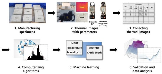
Figure 1.
The procedure of machine learning with thermal images.
2.2. Test Specimen
The test specimens were named according to the crack width (W) and depth (H), as listed in Table 1. The first letter, C, in the designation stands for crack; for example, C5-20 stands for a crack with width 5 mm and depth 20 mm. The configurations of the test specimens are illustrated in Figure 2. Macrocracks were selected in this study because of the detection system and the early stage of this research. The purpose of the system was to detect significant cracks in damaged structures rapidly and widely, using UAVs in disaster situations such as post-earthquakes [22,23,24,25,26]. Currently, this system aims primarily to detect macrocracks using thermal images and machine learning; after the investigation, the microcrack test specimens will be used to improve the detection system. To manufacture the test specimens, molds were fabricated. After filling the concrete in the molds, polymer pieces of equal size to the cracks were installed at the planned crack locations with easily detached thin wax. The polymer pieces were fabricated using a 3D printer, and the strength of the concrete in the specimens was 24 MPa.

Table 1.
Name of test specimens.
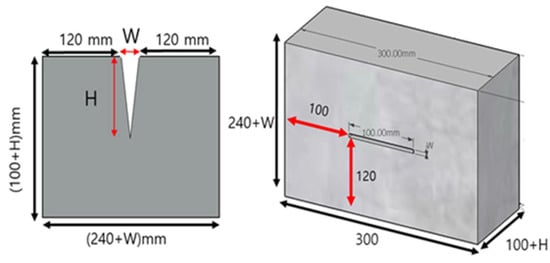
Figure 2.
Configuration of test specimens.
2.3. Test Setup
Thermal images were obtained from test specimens located outdoors at 1–4 pm after the specimens were directly exposed to sufficient daylight. To gather 6439 thermal images, the test was repeated over several months. The performance of a thermal camera located outdoors can be influenced by several parameters such as air temperature, humidity, illumination, cracks, and concrete surface temperature; the thermal images were therefore collected with those parameters set for machine learning. The air temperature ranged from −1.8 °C to 37.8 °C. In addition, humidity and illuminance ranged from 3.1% to 74.3%, and from 3200 lux to 91,810 lux, respectively. The test setup is shown in Figure 3, where the distance between the thermal camera and specimen was 5 m, which was determined by the minimum shooting distance of the UAV. This was because the proposed method aimed to rapidly detect the macrocrack at the unapproachable area using a UAV. The location and angle of the thermal camera towards the specimens were always fixed because the UAV with GPS can obtain ortho-thermal images with flight path planning in advance. In addition, the thermal camera was installed in the UAV instead of a normal camera with special modules. The professional thermal camera was an FLIR T530 [27], whose specifications are listed in Table 2. From the thermal images obtained, the raw data in the crack and surfaces were extracted at each temperature per pixel using environmental parameters. The surface temperatures at the upper and lower parts of the crack were measured because the surface conditions of concrete have more influence than the other environmental parameters. In addition, the specimen depth was decided by the previous studies [22,23,24,25,26] to avoid the rear surface effect on the crack or surface temperatures.
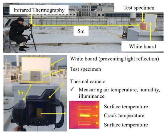
Figure 3.
Test setup.
Table 2.
Specification of the thermal camera [27].
2.4. Test Results
An example of the thermal images obtained is shown in Figure 4. The minimum pixel size of the thermal camera was 6.55 mm when the distance between the camera and specimen was 5 m. There was no issue with measuring the cracks of the specimen in this study, where the minimum width was 10 mm, as shown in Table 1. Because the test specimen was exposed to daylight before the test, the crack temperatures were higher than the surface temperatures. Light passed through the crack and was repeatedly reflected inside the crack. In contrast, light was reflected only once at the surface of the test specimen. Therefore, crack temperatures are higher than surface temperatures. The factors affecting the difference between crack and surface temperatures are environmental parameters, such as air temperature, humidity, and illuminance during the test. An example of the three-dimensional (3D) temperature distribution at the crack is shown in Figure 5, where the differences between the crack and surface temperatures are clearly shown. The shape of the temperature distribution at the crack was similar to that of the crack. An example of raw data with the parameters is presented in Table 3.
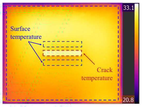
Figure 4.
Example of thermal images.
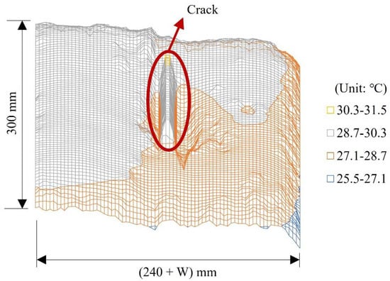
Figure 5.
Example of 3D visualization for temperature distribution at the concrete surface.
Table 3.
Example of raw data.
3. Data Analysis Result and Discussion
3.1. Parameter Information
The total number of data points was 6940, and all data were used for analysis. The statistical information and normal probability distributions of the data are shown in Figure 6 and Table 4. Standardization datasets were used to improve machine-learning performance. The crack depth was the target value for machine learning, whereas the others were input values.
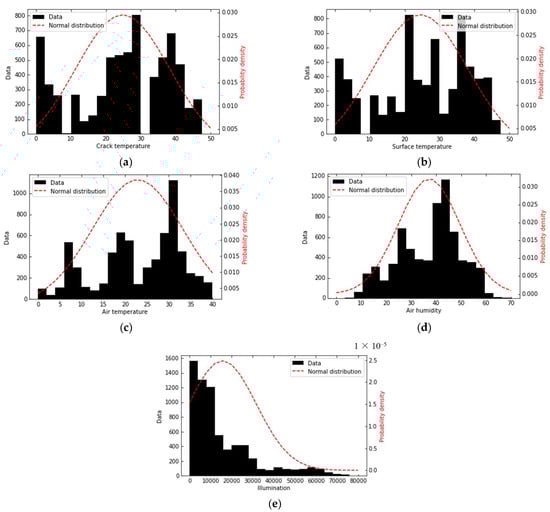
Figure 6.
Normal probability distribution: (a) crack temperature; (b) surface temperature; (c) air temperature; (d) air humidity; (e) illuminance.
Table 4.
Statistical information.
3.2. Machine Learning
This study used four machine-learning algorithms (decision tree, extremely randomized tree, extreme gradient boosting, and AdaBoost), because the previous study [19] used other machine-learning techniques (multilayer perceptron, random forest, gradient boosting, and AdaBoost) and suggested that AdaBoost could efficiently predict crack depth using thermal images. To prevent overfitting, cross-validation was conducted as a resampling procedure used to evaluate machine learning on a limited dataset. k-fold cross-validation, which partitioned the dataset into two groups (training and test), was selected [28]. Machine learning used the training group to analyze data and the test group for verification. The decision tree (DT) algorithm [29] classifies the data using criteria based on data features and structures the classification into a tree shape. Decision making is provided by the classifier function, and the subgroups are repeatedly divided until they match the target data. For example, the specific classifier for performing binary classification was selected, such as where the crack temperatures of the specimen with a 20 mm crack depth were over 30 °C when the air temperatures were over 25 °C. Then, the 25 °C air temperatures could be the first classifier to estimate the crack depth. However, to prevent the overfitting and the wrong estimation flow with complicated classifiers, selection was applied. From multiple and repeated classifiers, the decision tree algorithm estimated the crack depth. As the extremely randomized tree (EXT) [30] is an advanced random forest algorithm, overfitting rarely occurs. The subsamples of the data features are randomly selected, and the algorithm trains the optimal estimators. The EXT algorithm uses the entire training group for the training estimator, whereas the random forest uses only the extracted data. To estimate the crack depth, parameters were randomly selected without information gain. For example, 25 °C air temperature was randomly selected as the feature and the optimal estimators were calculated. After that, various features were randomly selected, and the optimal estimators were calculated to estimate the crack depths. As extreme gradient boosting (XGB) [31] is developed from the gradient boosting algorithm with classification and regression trees. The training speed of XGB is much faster than gradient boosting. The main feature of XGB is the regularized loss function to prevent overfitting, which can reduce the feature size and simplify training. Therefore, XGB can be used when data and situations are complicated. For example, several decision trees, such as the mentioned example in the DT, were combined and assigned their weights. The difference between the DT and XGB, is whether using sampling data or weighted sampling data. AdaBoost (AB) [32] is similar to the gradient boosting algorithm except for the weight factors. AB grades the weight factor for the misclassification data to apply to the next decision-making iteration, which can reduce the training duration and improve the accuracy. Therefore, AB can be applied to complicated situations with large data; however, the computation cost is high. For example, the crack temperatures of the specimen with a 20 mm crack depth were over 30 °C when the air temperatures were over 25 °C. The errors of this classifier were calculated, and this weighted data affected the second classifier and this procedure was repeated to derive the best estimation.
3.3. Results and Discussions
To evaluate the performance of the machine learning, five indicators, training and test scores, ±1 and 2 mm accuracies, and mean absolute percentage error (MAPE), were calculated. The training and test scores were evaluated using the coefficients of determination (R2train, R2test) using Equation (1).
where R2 is the coefficient of determination, SSR is the sum of squares related to regression, SST is the total sum of squares, yi is the real crack depth of the i-th data, ti is the estimated crack depth of the i-th data, is the average of the real depth, is the average of the estimated depth, and n is the number of data.
The coefficients of determination ranged between 0 and 1. If the value approaches zero, the correlations between the real and estimated cracks are irrelevant to each other. By contrast, if the value approaches 1, the correlation between the real and estimated cracks is relevant to each other. Generally, training scores are higher than test scores; when the difference between them is large, machine learning is overfitted. Next, accuracies of ±1 and 2 mm (acc1, acc2) were evaluated using Equation (2). This indicates the possibility of developing microcracks.
where acc is the accuracy, Ntrue is the number of estimated data points within the allowable errors, and n is the number of data points.
The mean absolute percentage error (MAPE) is a non-dimensional indicator for evaluating errors and an improved version of the root mean square error (RMSE) that does not consider size-dependent errors. MAPE can be expressed as follows:
where MAPE is the mean absolute percentage error, n is the number of data, yi is the real crack depth of the i-th data, and ti is the estimated crack depth of the i-th data.
MAPE should be set between 0 and 1. If the value approaches zero, the performance of the machine-learning algorithm is satisfactory. The machine-learning results for the aforementioned indicators are listed in Table 5. Based on the training and test scores, all algorithms except DT can be used for detecting macrocrack depths; the test score for DT is too low to effectively predict crack depths. DT showed lower scores because it is a single learner, whereas the other algorithms had several weighted learners to predict the crack depths. In addition, the test score of AB was the highest because of the weight factor of the misclassification data for the next decision. In terms of accuracy, only the AB algorithm has the possibility of detecting microcracks. However, XGB and AB can be selected for detecting macrocracks when considering MAPE because the MAPE of the EXT was quite high and even higher than DT. The difference between XGB and AB is the random classification of XGB and weighted factor for the misclassification data of AB. Therefore, random classification should be helpful in detecting macrocrack depth because the parameters showed a complicated correlation with the crack depth, not random correlation.
Table 5.
Machine-learning results.
4. Data Bias Analysis Result and Discussion
4.1. Data Bias Analysis
In this section, we discuss ways to prevent data bias and evaluate its effects using three bias prevention models: principal component analysis, singular value decomposition, and independent component analysis. A change in features may cause changes in other features because of covariation.
Principal component analysis (PCA) [33] is a technique used to evaluate the covariation of numerical variables, which selects smaller variable groups than the number of numerical variables. The principal component (Zi) can be obtained by multiplying the variables (Xi) by the weight values (wi,n) in the n-th data feature as follows:
where Zi is the principal component, wi,n is the weight, Xi is the variable, and i is the number of variable groups (=1, 2, …, k, k ≤ n).
To investigate the data bias for the crack depth, six principal components were used: crack, surface and air temperatures; humidity; illuminance; and crack width. The component with the highest weight value, when considering the six principal components, was the crack temperature.
Singular value decomposition (SVD) [34] can be presented in any matrix M, which is decomposed into three matrices, as follows:
where U is an m × m unitary matrix, Σ is an m × n diagonal matrix, V is an n × n unitary matrix, and VT is the conjugate transpose of V.
Matrix M is a real-valued data matrix; the columns represent samples, and the rows indicate the features. This technique finds the standard axis to make an average of rows zero similar to the PCA, and the axis with the largest value is decided as the matrix U. SVD is an efficient technique for most datasets, although it focuses on variance, and it is difficult to understand strongly nonlinear data.
Because PCA [35] creates orthogonal principal component vectors by extracting the principal components, the principal components are independent of each other. However, principal components that have no correlation, in fact, would not be independent of each other. To solve this limitation of PCA, independent component analysis (ICA) was developed to classify multidimensional data into independent components.
4.2. Analysis Results and Discussions
To evaluate the data bias analysis, three techniques, PCA, SVD, and ICA, were used with six parameters. The machine-learning algorithms for each technique show five performance indicators, as presented in Table 6. The value of several indicators decreased compared to the results in Table 5, whereas others remained almost unchanged. The reason for the decrease in the indicators was the data loss caused by the techniques used to classify the data groups. The performance of the SVD technique was better than that of the others for all algorithms, meaning that the correlation between crack depths and the six parameters was not random, and could be defined as simple non-linear relations. It is significant that the training scores of XGB with all techniques were excessively overestimated because their results were overfitted. However, this model has the potential to be developed for microcrack detection with accuracies up to ±1 and 2 mm, if the XGB can be controlled and prevented from overfitting. In addition, unlike DT and EXT, AB with PCA and ICA showed excellent performance in detecting macrocracks and development possibilities for detecting microcracks. PCA should be helpful for detecting microcracks in the XGB and AB. From a previous study [26] and the results of this study, AB is the best algorithm for detecting macrocracks. If overfitting can be prevented, XGB can also be used to detect macrocracks. For further studies on detecting microcracks, AB and XGB with PCA will be the best algorithms.
Table 6.
Data bias analysis.
5. Conclusions
This study proposes a method for predicting macrocrack depths in concrete using thermal images and machine learning. Using the same test setup, 6490 thermal images were obtained over several months for artificial crack specimens with known crack widths and depths, with exposure to environmental parameters such as air temperature, humidity, and illuminance. These provided the input data for the machine learning. To detect the macrocrack depth, four machine-learning methods, DT, EXT, XGB, and AB, were selected, and data bias analysis was conducted using PCA, SVD, and ICA. Similar to a previous study, the AB algorithm was found to be the best machine-learning algorithm, with or without data bias techniques. However, XGB can also be an excellent machine-learning method if it prevents overfitting. To evaluate the development possibilities of detecting microcracks in further studies, accuracies up to ±1 and 2 mm were obtained. Based on these accuracies, AB and XGB with PCA can be used to detect microcracks. In the case of XGB, overfitting must be prevented, as in a larger test dataset. The proposed concrete crack depth prediction method using thermal images and machine learning is expected to be actively used when rapid structural safety assessments are needed. For example, if a strong earthquake occurs in a city, the structural safety of numerous buildings in the city should be rapidly investigated. In addition, the proposed method with UAVs is expected to be applied to infrastructure or buildings where human access is impossible, such as nuclear facilities and irregular or tall buildings.
Author Contributions
Conceptualization, M.J.P., A.J., and Y.K.J.; methodology, M.J.P. and Y.K.J.; software, J.K., S.J., and J.B.; validation, M.J.P., J.B., and Y.K.J.; formal analysis, M.J.P., A.J., and Y.K.J.; investigation M.J.P., J.K., A.J., and Y.K.J.; resources, M.J.P., J.B., and Y.K.J.; data curation, M.J.P., J.K., S.J., A.J., J.B., and Y.K.J.; writing—original draft preparation, M.J.P., J.K., S.J., and Y.K.J.; writing—review and editing, M.J.P. and Y.K.J.; visualization, M.J.P., J.K., S.J., and J.B.; supervision, M.J.P., J.B., and Y.K.J.; project administration, M.J.P., A.J., and Y.K.J.; funding acquisition, Y.K.J. All authors have read and agreed to the published version of the manuscript.
Funding
This work was supported by a National Research Foundation of Korea (NRF) grant funded by the Korean government (MSIT) (No. NRF-2021R1A5A1032433 and NRF-2020R1A2C3005687). The authors are grateful to the authorities for their assistance.
Data Availability Statement
Not applicable.
Conflicts of Interest
The authors declare no conflict of interest.
References
- Aggelis, D.G.; Shiotani, T.; Polyzos, D. Characteristics of surface crack depth and repair evaluation using Rayleigh waves. Cem. Concr. Compos. 2009, 31, 77–83. [Google Scholar] [CrossRef] [Green Version]
- Lin, S.; Wang, Y. Crack-Depth estimation in concrete elements using ultrasonic shear-horizontal waves. J. Perform. Constr. Facil. 2020, 34, 04020064. [Google Scholar] [CrossRef]
- Sham, F.C.; Chen, N.; Long, L. Surface crack detection by flash thermography on concrete surface. Insight Non-Destr. Test. Cond. Monit. 2008, 50, 240–243. [Google Scholar] [CrossRef] [Green Version]
- Omar, T.; Nehdi, M.L. Remote sensing of concrete bridge decks using manned aerial vehicle infrared thermography. Autom. Constr. 2017, 83, 360–371. [Google Scholar] [CrossRef]
- Omar, T.; Nehdi, M.L.; Zayed, T. Infrared thermography model for automated detection of delamination in RC bridge decks. Constr. Build. Mater. 2018, 168, 313–327. [Google Scholar] [CrossRef]
- Kodikara, J.; Rajeev, P.; Rhoden, N.J. Determination of thermal diffusivity of soil using infrared thermal imaging. Can. Geotech. J. 2011, 48, 1295–1302. [Google Scholar] [CrossRef]
- Andrade, R.M.D.; Eduardo, A.C. Methodology for automatic process of the fired ceramic tile’s internal defect using IR images and artificial neural network. J. Braz. Soc. Mech. Sci. Eng. 2011, 33, 67–73. [Google Scholar] [CrossRef]
- Bauer, E.; de Freitas, V.P.; Mustelier, N.; Barreira, E.; de Freitas, S.S. Infrared thermography–evaluation of the results reproducibility. Struct. Surv. 2015, 33, 20–35. [Google Scholar] [CrossRef]
- Seo, H. Infrared thermography for detecting cracks in pillar models with different reinforcing systems. Tunn. Undergr. Space Technol. 2021, 116, 104118. [Google Scholar] [CrossRef]
- Chun, P.J.; Hayashi, S. Development of a concrete floating and delamination detection system using infrared thermography. IEEE-ASME Trans. Mechatron. 2021, 26, 2835–2844. [Google Scholar] [CrossRef]
- Feroz, S.; Abu Dabous, S. UAV-based remote sensing applications for bridge condition assessment. Remote Sens. 2021, 13, 1809. [Google Scholar] [CrossRef]
- Mandirola, M.; Casarotti, C.; Peloso, S.; Lanese, I.; Brunesi, E.; Senaldi, I. Use of UAS for damage inspection and assessment of bridge infrastructures. Int. J. Disaster Risk Reduct. 2022, 72, 102824. [Google Scholar] [CrossRef]
- Tong, X.; Guo, J.; Ling, Y.; Ying, Z. A new image-based method for concrete bridge bottom crack detection. In Proceedings of the 2011 International Conference on Image Analysis and Signal Processing, Wuhan, China, 21–23 October 2011. [Google Scholar]
- Nguyen, H.N.; Kam, T.Y.; Cheng, P.Y. A novel automatic concrete surface crack identification using isotropic undecimated wavelet transform. In Proceedings of the 2012 International Symposium on Intelligent Signal Processing and Communications System, New Taipei City, Taiwan, 4–7 November 2012. [Google Scholar]
- Zalama, E.; Gómez-García-Bermejo, J.; Medina, R.; Llamas, J. Road crack detection using visual features extracted by Gabor filter. Comput.-Aided Civ. Infrastruct. Eng. 2014, 29, 342–358. [Google Scholar] [CrossRef]
- Prasanna, P.; Dana, K.J.; Gucunski, N.; Basily, B.B.; La, H.M.; Lim, R.S.; Parvardeh, H. Automated crack detection on concrete bridges. IEEE Trans. Autom. Sci. Eng. 2016, 13, 591–599. [Google Scholar] [CrossRef]
- Shi, Y.; Cui, L.; Qi, Z.; Meng, F.; Chen, Z. Automatic road crack detection using random structured forests. IEEE Trans. Intell. Transp. Syst. 2016, 17, 3434–3445. [Google Scholar] [CrossRef]
- Chen, J.H.; Su, M.C.; Cao, R.; Hsu, S.C.; Lu, J.C. A self organizing map optimization based image recognition and processing model for bridge crack inspection. Autom. Constr. 2017, 73, 58–66. [Google Scholar] [CrossRef]
- Kim, H.; Ahn, E.; Shin, M.; Sim, S.H. Crack and noncrack classification from concrete surface image using machine learning. Struct. Health Monit. 2019, 18, 725–738. [Google Scholar] [CrossRef]
- Zhang, X.; Rajan, D.; Story, B. Concrete crack detection using context-aware deep semantic segmentation network. Comput.-Aided Civ. Infrastruct. Eng. 2019, 34, 951–971. [Google Scholar] [CrossRef]
- Zhu, J.; Song, J. An intelligent classification model for surface defects on cement concrete bridges. Appl. Sci. 2020, 10, 972. [Google Scholar] [CrossRef] [Green Version]
- Jeong, D.-M.; Batbayar, E.; Ju, Y.-K. Development of UAV-based building crack detecting system. In Proceedings of the Architecture & City in Seoul, Seoul, Korea, 26–27 April 2018. (In Korea). [Google Scholar]
- Lee, J.-H.; Jeong, D.-M.; Batbayar, E.; Ju, Y.-K. UAV & thermography module-based building crack detecting system. In Proceedings of the Spring Annual Conference of AIK, Seoul, Korea, 26–27 April 2019. (In Korea). [Google Scholar]
- Bae, J.; Jang, A.; Park, M.J.; Lee, J.H.; Ju, Y.K. Assessment of concrete macrocrack depth using infrared thermography. Steel Compos. Struct. 2021. in review. [Google Scholar]
- Bae, J.; Lee, J.; Jang, A.; Ju, Y.K.; Park, M.J. SMART SKY EYE system for preliminary structural safety assessment of buildings using unmanned aerial vehicle. Sensors 2022, 22, 2762. [Google Scholar] [CrossRef] [PubMed]
- Kim, J.; Jang, A.; Park, M.J.; Ju, Y.K. Comparison analysis of machine learning for concrete crack depths prediction using thermal images and environmental parameters. J. Korean Assoc. Spat. Struct. 2021, 21, 99–110. (In Korea) [Google Scholar] [CrossRef]
- Teledyne FLIR. Available online: https://www.flir.com/products/t530/ (accessed on 20 March 2022).
- Rodriguez, J.D.; Perez, A.; Lozano, J.A. Sensitivity analysis of k-fold cross validation in prediction error estimation. IEEE Trans. Pattern Anal. Mach. Intell. 2009, 32, 569–575. [Google Scholar] [CrossRef] [PubMed]
- Safavian, S.R.; Landgrebe, D. A survey of decision tree classifier methodology. IEEE Trans. Syst. Man Cybern. 1991, 21, 660–674. [Google Scholar] [CrossRef] [Green Version]
- Geurts, P.; Ernst, D.; Wehenkel, L. Extremely randomized trees. Mach. Learn. 2006, 63, 3–42. [Google Scholar] [CrossRef] [Green Version]
- Chen, T.; He, T.; Benesty, M.; Khotilovich, V.; Tang, Y.; Cho, H.; Chen, K. Xgboost: Extreme gradi-ent boosting. R Package, version 0.4-2. 2015; 1, 1–4. [Google Scholar]
- Rätsch, G.; Onoda, T.; Müller, K.R. Soft margins for AdaBoost. Mach. Learn. 2001, 42, 287–320. [Google Scholar] [CrossRef]
- Abdi, H.; Williams, L.J. Principal component analysis. Wires Comput. Stat. 2010, 2, 433–459. [Google Scholar] [CrossRef]
- Klema, V.; Laub, A. The singular value decomposition: Its computation and some applications. IEEE Trans. Autom. Control 1980, 25, 164–176. [Google Scholar] [CrossRef] [Green Version]
- Hyvärinen, A.; Oja, E. Independent component analysis: Algorithms and applications. Neural Netw. 2020, 13, 411–430. [Google Scholar] [CrossRef] [Green Version]
Publisher’s Note: MDPI stays neutral with regard to jurisdictional claims in published maps and institutional affiliations. |
© 2022 by the authors. Licensee MDPI, Basel, Switzerland. This article is an open access article distributed under the terms and conditions of the Creative Commons Attribution (CC BY) license (https://creativecommons.org/licenses/by/4.0/).