Optimizing Moving Object Trajectories from Roadside Lidar Data by Joint Detection and Tracking

Abstract

High-resolution traffic data, comprising trajectories of individual road users, are of great importance to the development of Intelligent Transportation Systems (ITS), in which they can be used for traffic microsimulations and applications such as connected vehicles. Roadside laser scanning systems are increasingly being used for tracking on-road objects, for which tracking-by-detection is the widely acknowledged method; however, this method is sensitive to misdetections, resulting in shortened and discontinuous object trajectories. To address this, a Joint Detection And Tracking (JDAT) scheme, which runs detection and tracking in parallel, is proposed to mitigate miss-detections at the vehicle detection stage. Road users are first separated by moving point semantic segmentation and then instance clustering. Afterwards, two procedures, object detection and object tracking, are conducted in parallel. In object detection, PointVoxel-RCNN (PV-RCNN) is employed to detect vehicles and pedestrians from the extracted moving points. In object tracking, a tracker utilizing the Unscented Kalman Filter (UKF) and Joint Probabilistic Data Association Filter (JPDAF) is used to obtain the trajectories of all moving objects. The identities of the trajectories are determined from the results of object detection by using only a certain number of representatives for each trajectory. The developed scheme has been validated at three urban study sites using two different lidar sensors. Compared with a tracking-by-detection method, the average range of object trajectories has been increased by >20%. The approach can also successfully maintain continuity of the trajectories by bridging gaps caused by miss-detections.

1. Introduction

Over the last several decades, the number of vehicles in cities has been increasing greatly with the rapid development of urbanization, which has created more traffic issues and increased the challenges in traffic management [1]. By providing trajectory-level data of road users, high-resolution micro traffic data (HRMTD) are more important to traffic safety and efficiency analysis than macro-level traffic information [2]. Vehicles are the main targets for HRMTD acquisition. Detecting vehicles and obtaining their dynamics and other information is a critical operation to create HRMTD [3]. Moreover, emissions from on-road vehicles are widely regarded to be the main source of air pollution in urban areas [4]. The study of vehicle emissions is therefore an important aspect for improving air quality. The fundamental step to conduct vehicle emission study is to identify vehicles and capture their dynamics. According to recent research, tracking of road users is the fundamental means to acquire HRMTD [3,5,6]. Video cameras and 3D lidar sensors are predominant devices to implement object tracking since traditional traffic sensors such as loop detectors mainly provide macro traffic data including traffic flow rates, average speeds, and occupancy [7]. Visual information from video cameras is richer, but the level of data accuracy is decreased by image distortion and resolution. Moreover, optical cameras are easily affected by illumination [8]. Panoramic 3D lidar sensors scan the 360°surroundings at a high frequency. Objects in the scanning area can thereby potentially be detected and tracked directly in 3D with high spatial accuracy and temporal resolution. Moreover, with the ongoing development of lidar technology and increased ubiquity, the cost of such sensors has dramatically decreased in recent years; therefore, such sensors are increasingly being adopted in the field of traffic monitoring [9].

Roadside laser scanning systems can facilitate the generation of HRMTD. Most existing roadside lidar-based object tracking studies are based on a tracking-by-detection strategy. Firstly, moving points in the raw lidar data are segmented from the background. Secondly, these moving points are clustered into small groups. Every group represents an individual road user. Thirdly, vehicles are extracted either by locating the lanes which vehicles occupy [10], or by vehicle and non-vehicle classification among all determined clusters [8,11]. Global Nearest Neighbor (GNN) [10] and Kalman filtering (KF) [2] are commonly used methods in the final stage, namely vehicle tracking. It is acknowledged that points on the objects being scanned become sparser when the objects are further from the sensor; therefore, objects in the far scanning field become ‘low-observable’ because of indistinguishable shapes. Additionally, occlusions from other objects or from the target itself are common issues in object tracking from roadside laser scanning systems. The clusters under occlusions are defected or totally missing. The absence of detections is highly likely to occur in the above two situations. Tracking will thereby be affected in the tracking-by-detection procedure: the coverage of object trajectories will be decreased and/or the trajectory be interrupted.

The body of literature related to mitigating the dependence of tracking on detection in roadside laser scanning systems is quite small. There are normally two strategies adopted among the reported studies: (1) simultaneous detection and tracking; (2) tracking before detection. In the first strategy, detection and tracking are either simultaneously performed by transferring the points on the moving objects into the space-time coordinate system [9] or improving detection performance using the information provided by tracking [12]. In the second strategy [13,14], as part of the preprocessing, tracking is implemented before knowing the identity of the clusters. The following classification is performed at a trajectory level to utilize as much traffic information as possible. The aforementioned research has mitigated the disadvantages of the traditional tracking-by-detection methods. Nevertheless, work in [12,13,14] has mainly focused on object classification, regarding tracking as one of the pre-processing operations [13,14], or the means to improve detection ability [12]. Thus, there is still scope for further research into tracking. Although tracking plays a vital role in [9], it focuses only on a single class (pedestrians), which is insufficient for large scale HRMTD acquisition. In addition, there are difficulties transferring the methodology to other classes such as vehicles.

Intending to enhance tracking performance to acquire higher quality HRMTD, a Joint Detection And Tracking (JDAT) scheme is proposed in this paper. Moving points are firstly extracted and road users are obtained via clustering. A tracker combining an Unscented Kalman Filter (UKF) [15] and a Joint Probabilistic Data Association filter (JPDAF) [16] is implemented on the obtained road user clusters without knowing the exact classes. In the meantime, vehicles and pedestrians are detected by PointVoxel-RCNN (PV-RCNN) from the moving point clouds. The trajectories are classified into vehicles and pedestrians by identifying the representatives from the object detection results. The main objectives of the research reported in this paper are as follows:

(1)

Occlusions and data sparsity are the main challenges of roadside lidar data, causing interruptions and shortened range of object trajectories. Thus, the first objective of this paper is to increase object tracking ranges and improve trajectory continuity for enhanced information extraction.

(2)

As there are different kinds of on-road objects, it is useful to learn how object category affects the maximum tracking range, which can also be influenced by the number of laser beams on the lidar sensor; therefore, the second objective of this paper is to investigate how the object types/sizes and number of lidar beams practically affect the trackable ranges in roadside lidar systems.

To achieve the above objectives, the proposed JDAT scheme keeps small segments that are caused by occlusions or long distances for tracking so that the tracking ranges can be increased and the trajectory continuity can be improved. The maximum tracking ranges of four different types of on-road objects (bus, car, van, pedestrian) have been assessed. It has also been proven that a higher number of beams can expect a longer tracking range in general, via the comparison of two different lidar sensors (RS-LiDAR-32 and VLP-16).

2. Related Work

Tracking-by-detection is widely applied in current object tracking studies based on video images, on-board lidar, as well as fixed lidar. The first section gives a brief review of roadside lidar-based object tracking with tracking-by-detection schemes. Tracking-before-detection is another object tracking strategy which has not been fully explored, especially in the field of laser scanning. The related work is summarized in the second section.

2.1. Tracking-by-Detection

Most current lidar-based object tracking studies utilize a tracking-by-detection strategy in which objects are detected before they are tracked. According to the methodology exploited in object detection, existing tracking-by-detection related studies can be divided into two subsequent categories.

In the first category [2,8,10,17,18], object detection is generally realized by an object detection framework containing moving point detection, clustering and classification. Object tracking is conducted by filtering methods. Several representative studies are summarized as follows:

In the study presented by Zhao et al. [2] the background filtering algorithm involves frame aggregation, point statistics, threshold learning, and real-time filtering. In the clustering stage, a modified Density-Based Spatial Clustering of Applications with Noise (DBSCAN) clustering algorithm with adaptive MinPts value and searching radius is developed. After clustering, a reference point is selected to represent each cluster, which will be used in the later procedures. A classification model based on BP-ANN is developed to distinguish pedestrians and vehicles in the detection range. A discrete KF is used in the tracking stage.

In the work of Zhang et al. [8] moving points are extracted by a Max-Distance algorithm in the first instance. These are then clustered into individual objects via a Euclidean Cluster Extraction algorithm. These objects are later classified into vehicles and non-vehicles by traditional classification methods. A tracker composed of UKF and JPDAF is adopted in the subsequent tracking stage.

Wu [9] developed an automatic 3D-Density-Statistics-Background-Filtering algorithm to filter the background from the scene. A unique operation after background filtering is lane identification, which aims to restrict the operation area to lanes. Consequently, the remaining foreground points only belong to vehicles so that classification is no longer needed. Subsequent procedures mainly comprise vehicle clustering, for which DBSCAN is adopted, and continuous vehicle tracking. To realize continuous vehicle tracking, a point is selected for each vehicle cluster and the GNN algorithm is applied to track the same vehicle in different frames.

In the second strategy [19,20,21,22,23], objects are detected directly from original point clouds by deep learning technologies and then tracked using either filtering or deep learning algorithms.

In two typical studies of the second strategy [19,20], two state-of-the-art 3D detectors [20,21] are explored in the detection stage to obtain bounding boxes. Pre-trained models from the KITTI 3D object detection benchmark [24] training set are adopted. In the tracking stage, a 3D KF predicts the state of associated trajectories from the previous frames to the current frame. Thereafter, a data association module based on the Hungarian algorithm [25] matches the predicted trajectories from the KF and detections in the current frame. Afterwards, the KF updates the state of trajectories based on the matched detections. Finally, a module is designed to manage the birth and death of the detected objects.

The tracker used in the above work was adopted by Shi, et al. [23] to obtain object IDs of the 3D boxes generated from lidar data by an off-the-shelf 3D object detector, PV-RCNN. SECOND was used as the 3D object detector in the proposed tracking system, considering the detection speed and effect, by Wang et al. [26] A 3D KF was used in the subsequent tracking module. Different from the above work, in which filtering algorithms were adopted at the tracking stage, a deep learning based-method was used for data association by Weng et al. [27] More specifically, a Graph Neural Network was applied to multi-object tracking for the first time. Moreover, a novel feature interaction mechanism was introduced to make the affinity matrix more discriminative.

2.2. Tracking-before-Detection

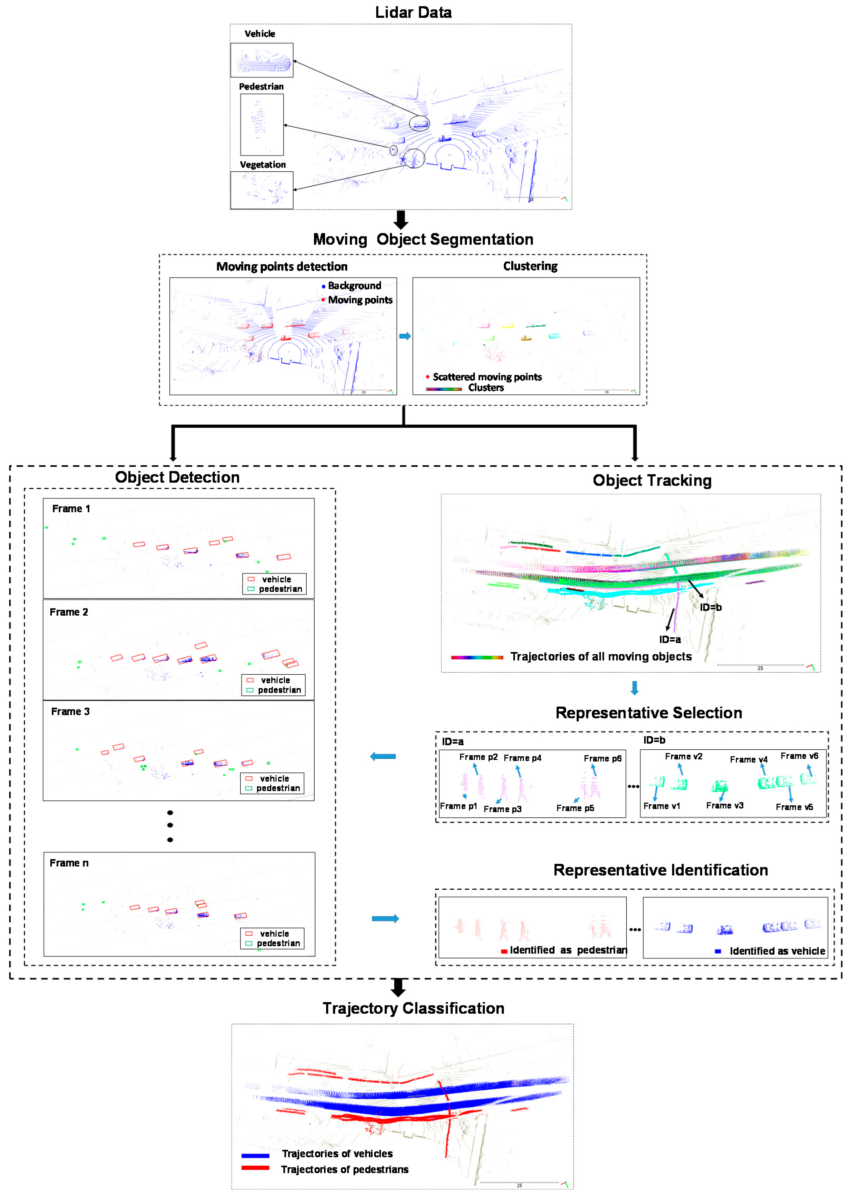
Tracking-before-detection is normally adopted to track low-observable objects which are easily overlooked in traditional tracking-by-detection schemes, or to reduce the complexity or remove the constraints on certain object categories in existing technologies.

As described by Tong et al. [28] by making full use of the raw radar data, a tracking-before-detection strategy is suitable for the detection and tracking of low-observable objects. A classical Probabilistic Hypothesis Density filter, with a ‘standard’ multi-target measurement model, is proposed in this work to deal with the multi-target tracking-before-detection problem. Moreover, an efficient segmentation mask-based tracker, which associates pixel-precise masks reported by the segmentation, is presented by Ošep et al. [29]. This approach utilizes semantic information whenever available for classifying objects at track level, while retaining the capability to track generic unknown objects in the absence of such information. Mitzel and Leibe [30] proposed a novel tracking-before-detection method that can track both known and unknown object categories in very challenging video sequences of street scenes. Gonzalez et al. [31] raised a track-before-detect framework for multibody motion segmentation based on vehicle monocular vision sensors. The contribution of this work relies on a tightly coupled tracking-before-detection strategy intended to reduce the complexity of existing multibody structure from motion approaches. To remedy fragmented trajectories due to detection failures in the tracking-by-detection framework, a novel detection-by-tracking method that prevents trajectory interruption was proposed by Chen et al. [32] Based on this method, an object’s accurate 3D bounding box can be recovered according to the tracking results in the situation of occlusions and missed detections.

The aforementioned object tracking methods based on the tracking-by-detection strategy have been confirmed to be efficient in certain aspects; however, they are not qualified to provide more detailed HRMTD due to the negative influence from the object detection process. Moreover, although tracking-before-detection has great potential to detach tracking from detection, the current small number of approaches for either radar or video sensors cannot be directly applied to lidar sensors; therefore, there is still much potential for object tracking from laser scanning systems, especially roadside sensors.

3. Methodology

As shown in Figure 1, there are three main stages in the proposed methodology: segmentation as a pre-processing operation; tracking of all the moving objects; trajectory classification intended to categorize the trajectories into vehicles, pedestrians, and others. The three stages are explained as follows.

3.1. Segmentation

Moving points detection and clustering are two main operations to segment the moving objects from the original point cloud. Moving points are detected by the Max–Distance strategy [9]. According to the operating principle of the laser scanner, each laser beam rotates in a circle repeatedly with a proper angular resolution [33]. A point named as $P_{i\times j}$ is obtained when the $i_{th}$ laser beam is directed at the azimuth angle $j$. The distance of this point to the laser scanner can be denoted as $D^{i\times j}$. The laser beam is not supposed to pass through the static background ($R_b^{i\times j}$); therefore, the furthest point at $(i,j)$ with the distance of $D_{\max }^{i\times j}$ should locate at the background. If $D^{i\times j}$ < $D_{\max }^{i\times j}$, $P_{i\times j}$ is on a moving object ($R_m^{i\times j}$), as can be seen in Equation (1). The background of each test site is constructed by determining the furthest point at every location in $R^{i\times j}$. The construction is expected to be implemented during a certain time period when there are only a small number of moving objects.

$$P_{i\times j}\in \{\begin{array}{l}{{\displaystyle {{\displaystyle R}}_m^{i\times j},\hspace{0.17em}\hspace{0.17em}if\hspace{0.17em}D}}^{i\times j}<{{\displaystyle D}}_{\max }^{i\times j} \hspace{0.17em}\hspace{0.17em}\hspace{0.17em}\\ {{\displaystyle {{\displaystyle R}}_b^{i\times j},\hspace{0.17em}if\hspace{0.17em}D}}^{i\times j}={{\displaystyle D}}_{\max }^{i\times j}\hspace{0.17em}\hspace{0.17em}\end{array}\hspace{0.17em}\hspace{0.17em}i\in \hspace{0.17em}(1,2,\dots ,n),\hspace{0.17em}j\in (0,{360}^{\circ \hspace{0.17em}})$$

(1)

The Euclidean Cluster Extraction (ECE) algorithm is used to group points on the same moving object. One parameter that greatly matters in the clustering process is the minimum cluster size $S_1$. Small clusters with few points in the far scanning field are supposed to be maintained because the following object tracking step aims to associate all visible clusters in the scanning region so that tracking can continue to the maximum extent. According to the datasets exploited in this work, $S_1$ is set to 5. The ECE algorithm is illustrated in the following steps:

• Create a Kd-tree representation of the point cloud dataset, P.
• Set up an empty list of clusters, C, and a queue of points requiring processing, Q.
• For every point p_i in P, the following operations will be undertaken:

  (1)

  Add p_i to Q.

  (2)

  For every point p_k in Q, search the neighboring points in a sphere with radius r < d. Then check each neighboring point to see if it has already been processed, if not, add it to Q.

  (3)

  If all points in Q have been processed, add Q to C and reset Q to empty.

• Terminate when all the points in P have been processed and included in C.

3.2. Object Tracking

After segmentation, clusters belonging to the same object in successive frames are supposed to be associated to retrieve the trajectory. A tracker utilizing UKF as the initial function and JPDAF as the association algorithm is adopted in the tracking flow to provide trajectories of the objects. It is noteworthy that all the segmented moving objects are tracked without knowing the specific categories. The state and measurement equations are as Equation (2). The final state update equation is given as Equations (3) and (4).

$$\begin{array}{l}{x}_{k+1}=f(x_k,\hspace{0.17em}{u}_k,t)+w_k\\ z_k=h(x_k,\hspace{0.17em}t)\hspace{0.17em}+v_k\end{array}$$

(2)

A constant-velocity UKF is first initialized, which estimates the state of a vehicle by a nonlinear stochastic equation. In constant-velocity motion, the state vector of a vehicle is defined as $x=[x\hspace{0.17em};\hspace{0.17em}\hspace{0.17em}{v}_{x\hspace{0.17em}};\hspace{0.17em}y\hspace{0.17em};\hspace{0.17em}\hspace{0.17em}{v}_y]$.

Where $x_k$ is the state at step $k$; $f$ is the state transition function, $u_k$ is the control on the process. The motion may be affected by random noise perturbations $w_k$. $h$ is the measurement function that determines the measurements as functions of the state. Typical measurements are position and velocity or some functions of these, which can also include noise represented by $v_k$.

$$Z_k^i\hspace{0.17em}=h({\chi }_{k/k-1}^i)\hspace{0.17em}\hspace{0.17em}\hspace{0.17em}\hspace{0.17em}\hspace{0.17em}\hspace{0.17em}\hspace{0.17em}\hspace{0.17em}\hspace{0.17em}i=0,\dots ,\hspace{0.17em}2L$$

(3)

$${\widehat{{\rm X}}}_{k|k}={\widehat{{\rm X}}}_{k|k-1}+K_k{v}_k$$

(4)

In the UKF-JPDAF-based tracking procedure, the confirmation threshold, normally used to confirm a track and specified as [M, N], is critical to the tracking range. A track is confirmed if it recorded at least M hits in the last N updates. Thus, the first M-1 clusters of an object will not be assigned to the corresponding track based on the parameter definition. To avoid missing any potential targets, the confirmation threshold in this work is set to [1, 3].

Moving objects in this work mainly refer to vehicles, pedestrians, cyclists, motorcyclists, and false alarms (e.g., trees and bushes moving in wind). According to practice, trajectories of any false alarms should be relatively short; therefore, to reduce false alarms in the subsequent trajectory classification, trajectories with lengths shorter than a certain threshold L are removed after tracking.

3.3. Object Detection Based on PV-RCNN

Although traditional classifiers perform well when the clusters of targeted objects are extracted, selecting distinguishable hand-crafted features is a laborious task that somewhat depends on personal experience. Fortunately, the widely and fast developing deep learning technologies provide comprehensive features for the objects through learning mechanisms. PV-RCNN is a recently proposed 3D object detection network that has integrated the advantages of prevalent point-based methods and voxel-based methods. Moreover, according to Shi et al. PV-RCNN performs well using KITTI data [34] Considering that the difference between data used in KITTI and in this study is primarily the data density, it is anticipated that PV-RCNN will also work well here. More specifically, PV-RCNN is operated on the processed lidar scans containing only moving points in order to remove false alarms.

The PV-RCNN framework is trained end-to-end by the self-created training dataset with the training loss that is the sum of the following three losses: the region proposal loss $L_{rpn}$, keypoint segmentation loss $L_{seg}$, and the proposal refinement loss $L_{rcnn}$. The three losses are summed with equal loss weights. A Grid search algorithm is adopted in the training process to determine the optimum value for the most important hyperparameters such as batch-size, epoch and voxel-size [35].

The original PV-RCNN algorithm was trained by samples of three classes including cars, pedestrians and cyclists from KITTI data; however, in our case, cyclists are not considered as a single class because the number of occurrences in the collected lidar data is extremely small. Therefore, a two-class training dataset is created using the third-party point cloud labelling software, Supervisely [36].

3.4. Trajectory Classification

After tracking, clusters of the same object have been associated across successive frames; however, not all of them are needed in the trajectory classification process because they belong to the same category. Since larger clusters are more distinguishable than those with smaller sizes in a trajectory, they can act as representatives of the trajectory that will be fed into the classifier, such that the negative influence from the low-observable clusters can be minimized.

By identifying the categories of the representatives according to the results of object detection, the category of the corresponding trajectory can be determined. One attribute of the representatives is the ID of the original lidar frame from which the representative is extracted. As PV-RCNN is operated on frames that only contain moving points abstracted from the corresponding original lidar frame, the category of the representatives can be easily traced from the detection results by their frame IDs. If at least $p$ (a ratio) of the total number (n) of representatives are classified as one of the classes in the detection results, the trajectory is allocated into that class.

4. Experimental Results and Analysis

4.1. Datasets

The tests conducted in this research employ two different lidar sensors. The first is a RS-LiDAR-32, a panoramic instrument from RoboSense. The sensor has a scanning radius of up to 200 m and is designed for various applications such as autonomous vehicles, robotics, and 3D mapping. It has 32 laser beams and collects data at a speed of 640,000 pts/s. The scanning frequency is set to 10 Hz in our tests. It covers a 360° horizontal FOV and a 40° vertical FOV with 15° upward and 25° downward looking angles. The second sensor is a Velodyne VLP-16, with 16 laser beams and a maximum scanning range of 100 m. The vertical field of view of the instrument is 30° with 15° upward, and 15° downward, look angles. The scanning frequency is also set to 10 Hz in our experiments.

Three different study sites were chosen in Newcastle upon Tyne, UK, to test the proposed method under real-world traffic conditions. At the first site (Figure 2a), a RS-LiDAR-32 lidar sensor was setup along a straight road near a traffic light controlled pedestrian crossing. The lidar sensor was c. 4 m away from the first of two traffic lanes. At the second site (Figure 2b), a VLP-16 lidar sensor was set up at a road intersection. The lidar sensor was c. 4.5 m away from the first of multiple lanes. Study Site 3 was at a roundabout with busy traffic, where a VLP-16 was installed but with a shorter distance of c.2 m to the nearest lane (Figure 2c).

A dataset containing 3184 vehicles and 1563 pedestrians was created from 763 lidar frames collected at Study Site 1. 360 vehicles and 368 pedestrians from 63 frames composed the test split. The remainder of the dataset is divided into train split and validation split at a ratio of 7:3.

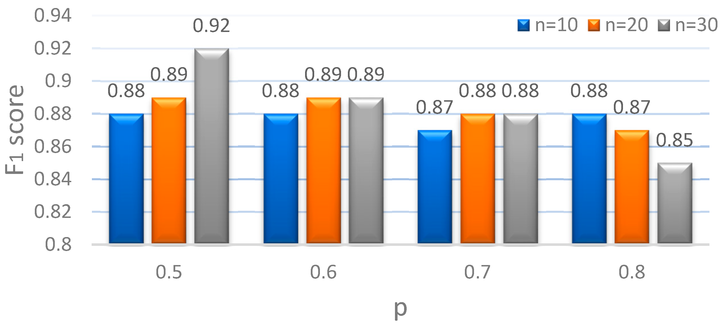
4.2. Experiment Settings

4.2.1. Segmentation

The background of each test site is constructed prior to moving point extraction. Background construction is normally conducted by successive frames in a certain time interval when the number of moving objects is as small as possible. In our experiments, for each of the three study sites, 100 successive frames in a quiet period were selected to perform background construction.

In clustering, there are three important parameters: the minimum cluster size S₁, the maximum cluster size S₂, and the minimum distance d between two clusters. At three study sites of this research, the minimum distance between two vehicles is around 1.5 m, and the minimum distance between a pedestrian and a vehicle is around 1.8 m; therefore, d is set to 1 m in the tests. The cluster size is dependent on the number of beams of the sensors, and thus needs to be adjusted for different sensors. According to comprehensive statistics, the largest vehicle cluster contains around 6000 points from RS-LiDAR-32, so S₂ = 6500. Since the point density is much lower from the VLP-16, the value is smaller: S₂ = 5500. Small clusters with few points in the far scanning field are supposed to be maintained because the following object tracking step is aimed to associate all the visible clusters in the scanning region so that tracking can be continued to the maximum extent. According to the datasets from three study sites, $S_1$ is set to 5.

4.2.2. Object Detection and Tracking

As for PV-RCNN, the entire network was trained with batch size 4, learning rate 0.01, for 100 epochs on a NVIDIA GeForce RTX 3090 GPU, which took around 8 h in terms of processing time.

Some important parameters in the tracking stage are specified in

Table 1. Parameter settings used in tracking stage.

Procedure	Parameter	Description	Setting	Basis of Setting
Initialization	Initialization threshold	Threshold to initialize a track	0.1	Default
	confirmation threshold	Threshold for track confirmation	[1, 3]	Experiment
Data association	Assignment threshold	Detection assignment threshold	[4 m, Inf]	Practice and empirical knowledge
Track management	Deletion threshold	Threshold for track deletion	[5, 5]	Default
	Length threshold	Threshold to delete a non-vehicle trajectory	3 m	Experiment and practice

. These parameters are involved in the three stages of tracking including initialization, data association, and track management. The description, setting, and justification for each parameter is shown in the table. ‘Initialization threshold’ is used to start a new track. If the association probability of a detection within the assignment gate is lower than the threshold, a new track will be generated. This parameter is usually set as a scalar in [0, 1]. In this study, the default value of 0.1 in the JPDAF algorithm was assigned to this parameter. ‘Confirmation threshold’ is a parameter to confirm a track and is normally specified as [M, N]. A track is confirmed if it records at least M hits in the last N updates. Thus, the first M-1 clusters of an object are not assigned to the corresponding track. To avoid missing any potential targets, the confirmation threshold in this study was set to [1, 3]. ‘Assignment threshold’ is the pivotal parameter in data association. It controls the range within which the detections are assigned to tracks, namely, the assignment gate. If the value is too small, some detections that should be assigned to a track might be overlooked. Otherwise, there will be false assignments. In this study, it was empirically set to 4 m, considering both the average vehicle speed and lidar sensor frame rate. There are two parameters in track management worth mentioning: the first is ‘Deletion threshold’, which is used to delete a track. It is normally set as [P, R], which means a confirmed track will be deleted if it is not assigned to any detection in P of the last R tracker updates. The default value in the JPDAF algorithm is [5, 5] and this value was adopted in this study. The other parameter is ‘Length threshold’, a parameter used to delete trajectories that do not belong to road users. It was set as 3 m according to experiments and practice.

4.2.3. Trajectory Classification

Further experimentation is necessary to determine the optimum parameters in trajectory classification. n is the number of representatives of a trajectory, whereas p is the ratio of representatives identified as vehicles to all the representatives. Six cases have been tested with different values (n = (10, 20, 30), p = (0.5, 0.6, 0.7, 0.8)) to decide the optimal n and p in terms of the classification performance of the trajectories which is measured by the F₁ score. According to Figure 3, the classification performance is optimum when n = 30 and p = 0.5.

4.3. Results and Analysis

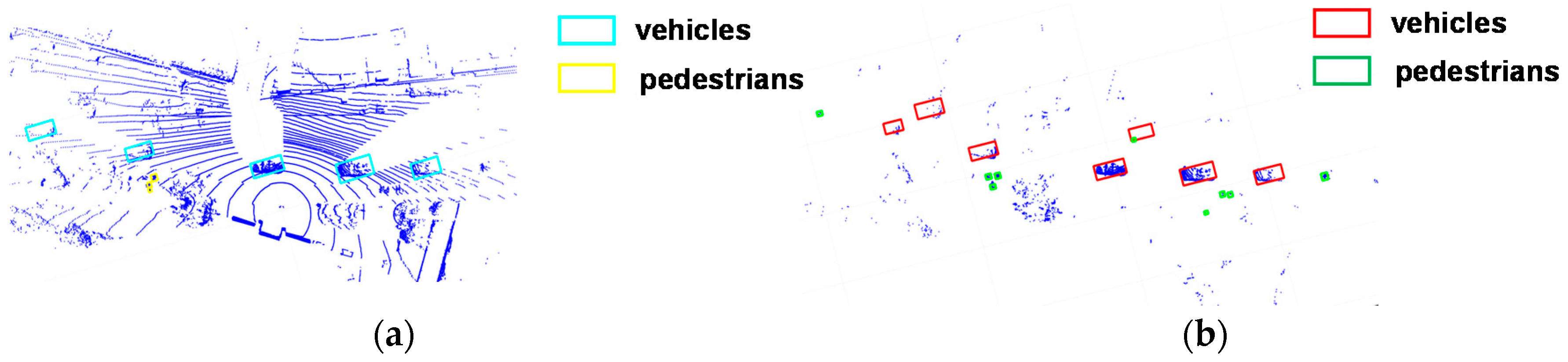
4.3.1. Detection Results

The results of PV-RCNN detection at Study Site 1 are shown in Figure 4 and

Table 2. Detection results from PV-RCNN.

Class	Total Number	Recall (%)	Precision (%)	F1 (%)
Vehicle	182	74.7	83.4	78.8
Pedestrian	146	72.6	65.4	68.8

. Recall, precision, and F₁ are adopted to evaluate the detection results. As can be seen from Table 2, F₁ of vehicle is 10% higher than that of pedestrian. There is no significant difference between recall values of the two classes, but the precision of vehicle is much higher than that of pedestrian. The worse results for pedestrians can be explained by the limitation of PV-RCNN, where an insufficient number of key points may harm the performance of objects with small sizes [33].

4.3.2. Trajectory Classification Results

The results of trajectory classification at Study Site 1 are shown in Figure 5 and

Table 3. Trajectory classification results by JDAT.

Class	Ground Truth	Recall (%)	Precision (%)	F1 (%)
Vehicle	20	70.0	82.4	75.7
Pedestrian	45	93.3	87.5	90.3

. There are 20 vehicle trajectories and 45 pedestrian trajectories obtained from the test data. Fourteen vehicle trajectories and 42 pedestrian trajectories have been correctly identified, resulting in recall values of 70% and 93.3%, respectively. The recall of a vehicle is low due to a misclassification of short trajectories that is located too far from the lidar sensor. The precision values of the two classes do not show big differences (82.4% of vehicle and 87.5% of pedestrian). The resulting F₁ of the vehicle is 75.7%, and of pedestrians, it is 90.3%.

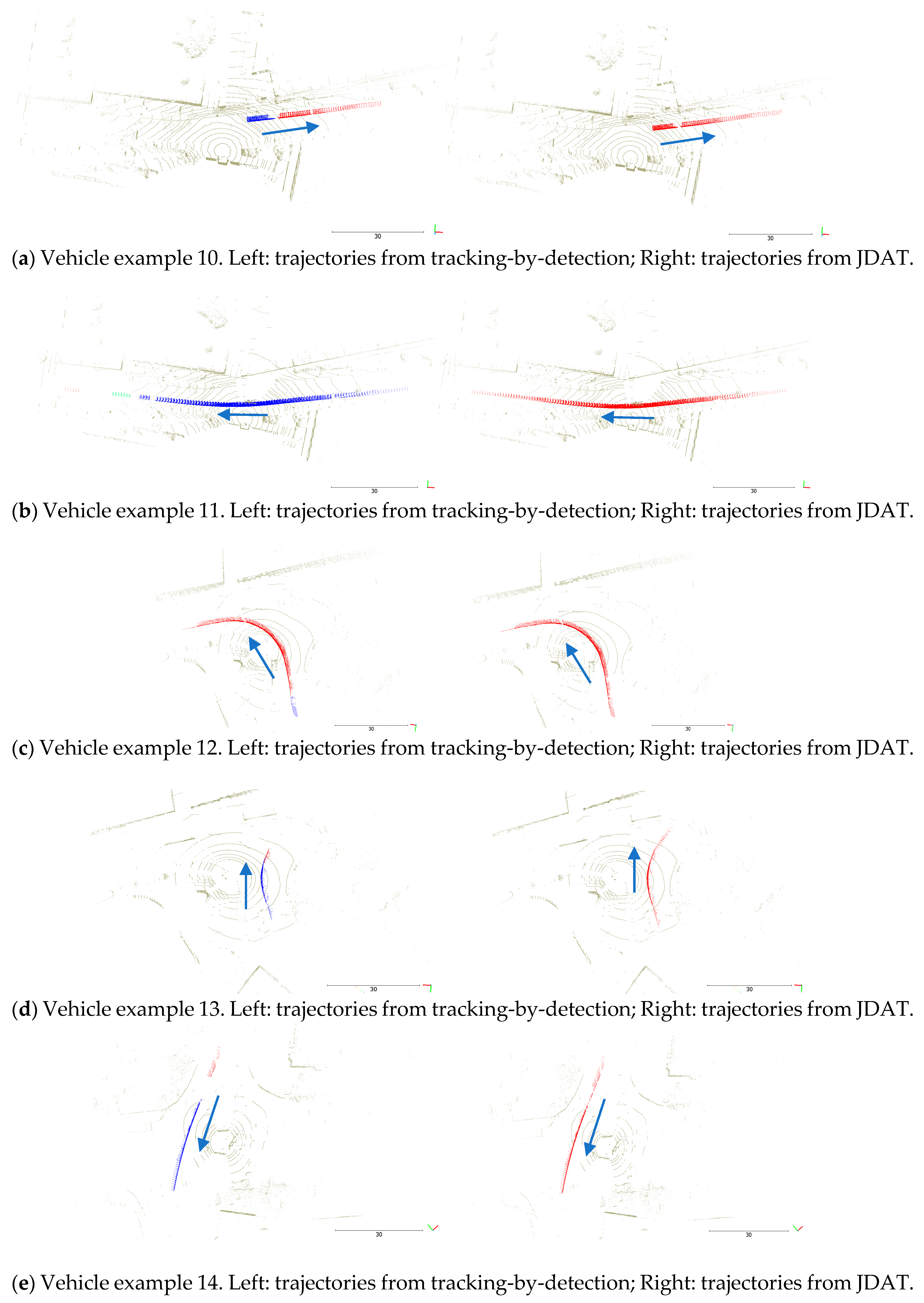
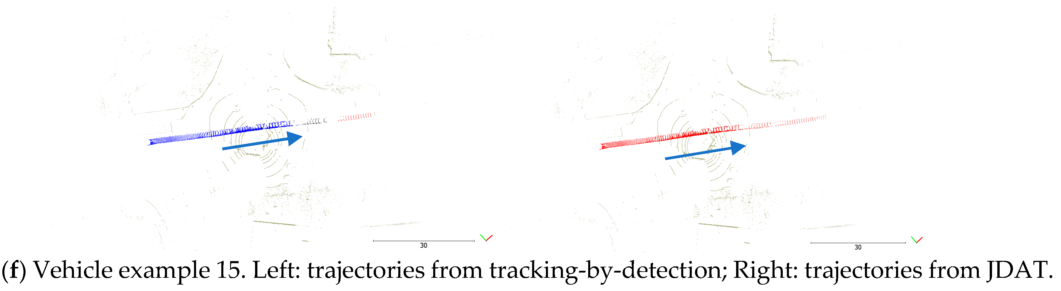
4.3.3. Comparison with Tracking-by-Detection Method

In tracking-by-detection methods, tracking is implemented after the objects are detected. Fifteen vehicle examples from three study sites are used to compare the tracking-by-detection method with the proposed method, with regard to both the range and the continuity of the trajectories. The maximum tracking ranges of two commonly used lidar sensors are further measured. The trajectories of these vehicle examples are shown in Figure 6 and Figure 7, and the statistics for ranges from the first nine examples are displayed in

Table 4. Comparison between the tracking-by-detection method and JDAT regarding the range of vehicle trajectories.

Study Sites	Vehicle Examples	Tracking-by-Detection			JDAT			Ground Truth			Comparison
		Start Frame	End Frame	N1	Start Frame	End Frame	N2	Start Frame	End Frame	N	N1/N (%)	N2/N (%)	N1/N2 (%)
1	1	777	849	73	743	849	107	741	849	109	67.0	98.2	68.2
	2	878	967	90	875	976	102	865	991	127	70.9	80.3	88.2
	3	4880	4971	92	4871	4979	109	4863	4996	134	68.7	81.3	84.4
2	4	4221	4274	54	4219	4284	66	4219	4302	84	64.3	78.6	81.8
	5	9110	9163	54	9100	9173	74	9100	9181	82	65.9	90.2	73.0
	6	9105	9162	58	9104	9174	71	9104	9185	82	70.7	86.6	81.7
3	7	0	20	21	0	34	35	0	34	35	60.0	100	60.0
	8	766	836	71	766	858	93	766	858	93	76.3	100	76.3
	9	926	977	52	926	987	62	926	987	62	83.9	100	83.9
Mean											69.7	90.6	77.5

.

• Ranges of the trajectories

Nine vehicles travelling across the entire scanning region are used to compare the two methods. For each vehicle, two trajectories are obtained from the two methods, individually. The start and the end frame of each trajectory are recorded in Table 4, as is the total number of frames the trajectory covers, which is denoted as N₁ for the tracking-by-detection method and N₂ for the proposed method. By checking the vehicle clusters from the original data, the corresponding ground truth (the number of frames is denoted as N in Table 4), which refers to the frames where the vehicle actually exists, can be obtained and regarded as the reference to compare the performance of two methods. N₁/N, N₂/N are used as indices for comparison.

From a qualitative perspective, Figure 6, trajectories from the proposed method appear longer than those from the tracking-by-detection method. The differences mainly lie in one (examples 1, 4, 6, 7, 8, 9) or two ends (examples 2, 3, 5) of the trajectories, which is in line with the assumption that low-observable clusters in the far field are very likely to be absent in the tracking-by-detection method. From a quantitative perspective, seen through the comparison results in Table 4, the proposed method outperforms the tracking-by-detection method, except for examples 2, 3, 4 and 6, as N₂/N can be over 90%, with several values even reaching 100%. The highest N₁/N value from the tracking-by-detection method is only 83.9%. The lowest N₁/N value is 60% in example 7, indicating that nearly half of the clusters are missing. Even though this is an extreme example, it indeed happens when the classifier is not properly trained. The proposed method is effective for improving such situations, as demonstrated where N₁/N has increased from 60% to 100% in example 7. The tracking ranges of nine vehicles are shown in Table 4, which further demonstrates the ability of JDAT to increase trajectory ranges. N₁/N₂ is used to directly compare the two methods. The average value of N₁/N₂ is 77.5%, which means the proposed method has increased the trajectory range by 22.5%.

• Continuity of trajectories

Six vehicle examples, denoted as vehicle examples 10–15 from the three study sites (10 and 11 from Study Site 1, 12 and 13 from Study Site 2, 14 and 15 from Study Site 3), are used to demonstrate that the proposed method has the ability to bridge the trajectory gaps caused by misdetections from the tracking-by-detection method.

In vehicle example 10 at Study Site 1, the trajectory from the tracking-by-detection method (left in Figure 7a) is chopped into two at the front end due to a short-time occlusion. Moreover, the corresponding trajectory from the proposed method (right in Figure 7a) is successive because clusters that are lost in the tracking-by-detection method are retained on the trajectory. In vehicle example 11 at Study Site 1, the trajectory from the tracking-by-detection method is divided into three parts from the rear end (blue, green and red in the left in Figure 7b) because some low-observable clusters are missing after vehicle detection. The problem is avoided in the proposed method and a continuous trajectory is generated (right in Figure 7b).

With regard to example 12 from Study Site 2 (Figure 7c), there is a slight occlusion at the beginning, and several affected clusters are overlooked in the detection stage in the tracking-by-detection method, resulting in interruption to the trajectory. Nevertheless, tracking proceeds smoothly from the beginning to the end in the proposed method. Vehicle example 13 at Study Site 2 is turning right. During a certain period, the vehicle clusters become too weak for the classifier due to self-occlusion. Thus, for a short moment, tracking using the tracking-by-detection method is suspended before the clusters are recovered. As a result, two trajectories are generated, seen as the left figure in Figure 7d. Although, there is no such problem in the proposed method because those low visible clusters are assigned to the trajectory directly in the tracking stage and they do not contribute to the subsequent trajectory classification.

Vehicles 14 and 15 from Study Site 3 both suffer from occlusions caused by other vehicles. As for vehicle 14, occlusion is severe, and the affected clusters only appear to be blurred boundaries. Accordingly, tracking is paused for around 1.5 s in the tracking-by-detection method (left in Figure 7e); however, there is no negative influence in the proposed method, as can be concluded from the integral trajectory in Figure 7e. In terms of vehicle 15 from Study Site 3, despite discontinuous occlusions, tracking is conducted without any resistance in the proposed method. Unfortunately, tracking in the tracking-by-detection method is interrupted twice, generating a trajectory that is cut into three pieces from the rear end (blue, black, and red in the right sub-figure in Figure 7f).

From the aforementioned comparisons based on 15 vehicle examples from three different study sites, it can be concluded that moving object trajectories from the JDAT method are more extensive than corresponding ones from the tracking-by-detection method. Moreover, the trajectory gaps resulting from the tracking-by-detection method can be stitched by the JDAT method, thereby improving the continuity of vehicle trajectories.

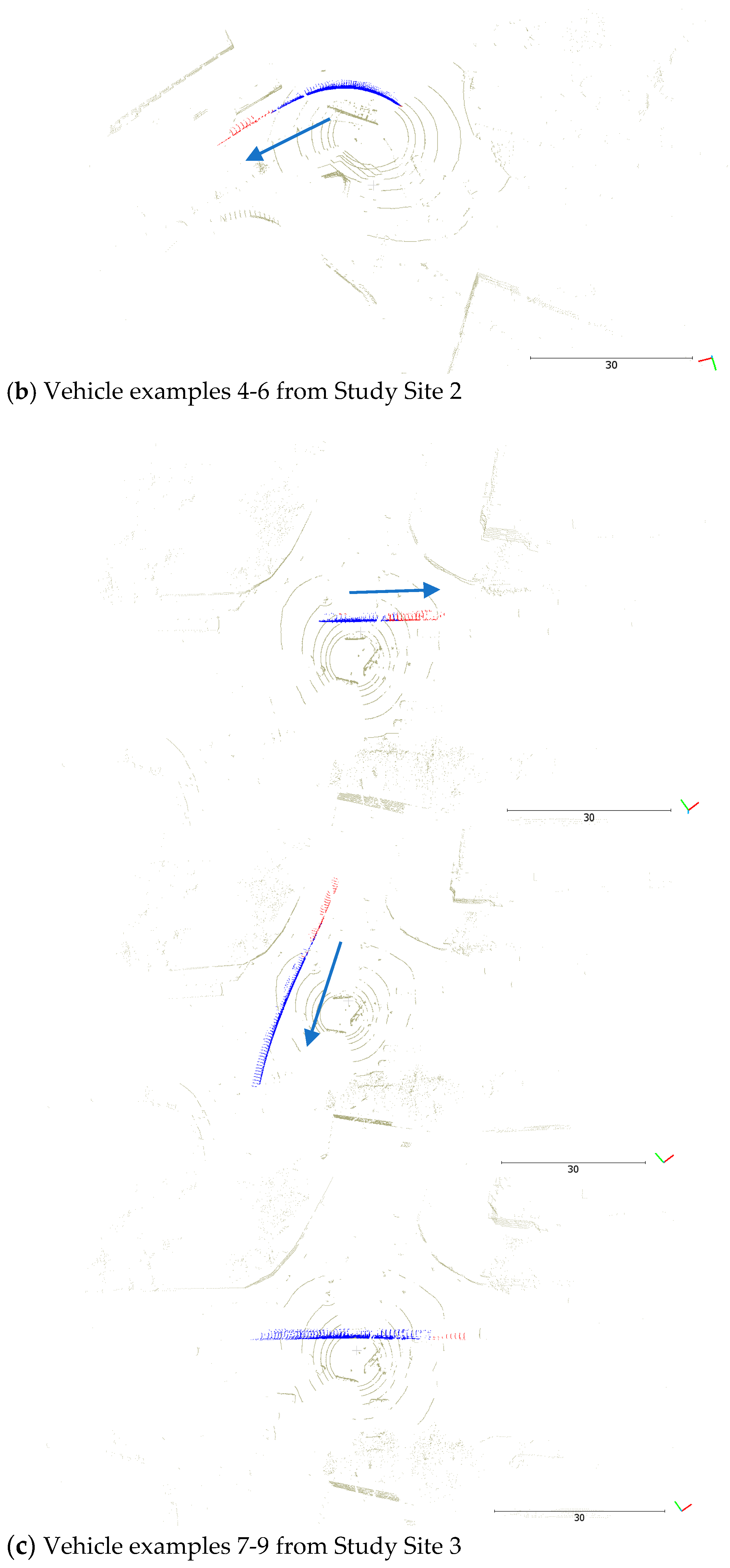
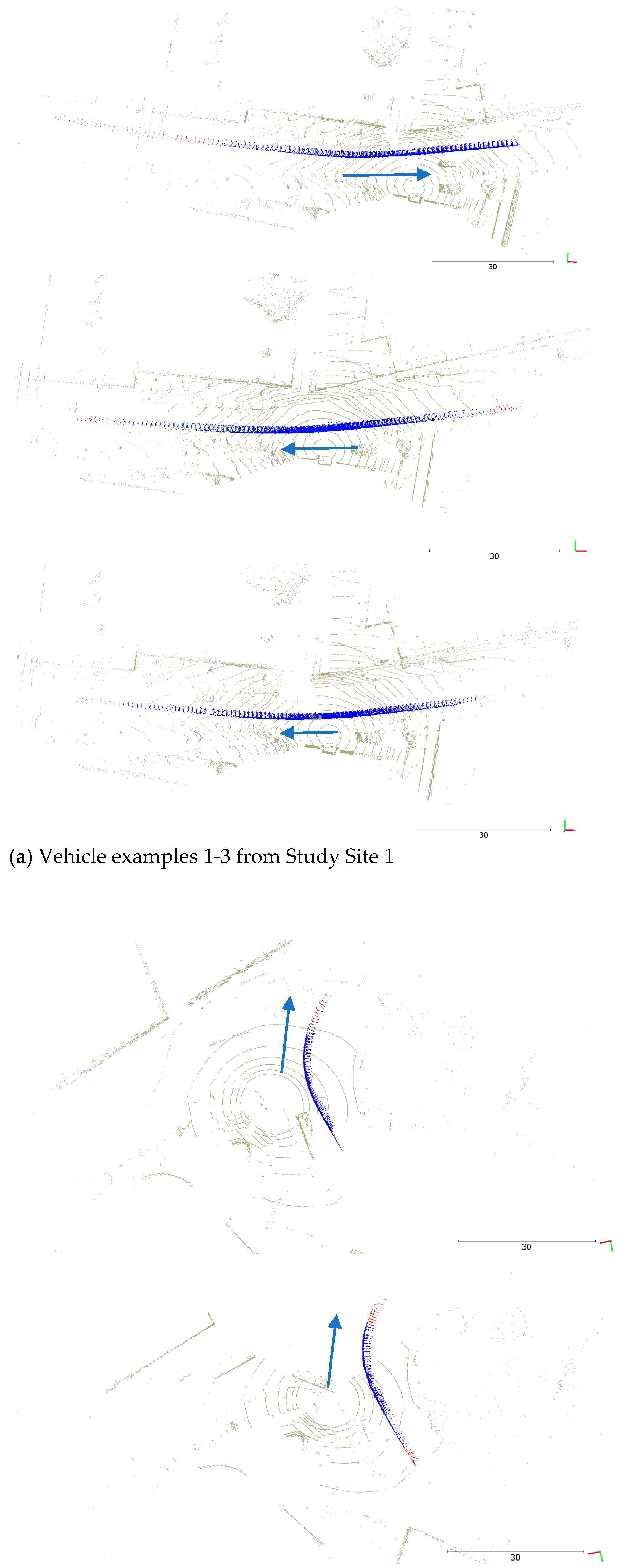
4.3.4. Maximum Tracking Range

It is of high practical significance to measure the maximum tracking ranges of different on-road objects. Object trajectories are classified into vehicles and pedestrians according to the detection results from PV-RCNN. Due to data limitations, it is impossible to further classify vehicles into different classes by PV-RCNN. A Random Forest classifier is thereby adopted to classify vehicles into buses, cars, and vans. Two lidar sensors installed at Study Site 1 and Study Site 2 are separately adopted to assess the maximum tracking ranges of the four adopted object categories.

The following observations can be obtained from

Table 5. Maximum tracking range of two different lidar sensors for different object categories.

Study Sites	Road Condition	Sensor Type	Maximum Tracking Range(m)
			Bus	Van	Car	Pedestrian
1	Straight section	RS-LiDAR-32	109.5	111.3	98.2	91.8
2	Intersection	VLP-16	112.39	49.26	38.16	48.50

:

• From a general perspective, the maximum tracking range of pedestrian is shorter than
• that of vehicles including bus, car, and van. At Study Site 1, the maximum tracking range of pedestrian is the shortest among all the categories because it has the smallest object size. Although, at Study Site 2, the maximum tracking range of pedestrian is longer than that of car because two pedestrians were walking together and were tracked as one object.
• In terms of vehicles, the maximum tracking range of car is shorter than that of van and bus due to smaller object size.
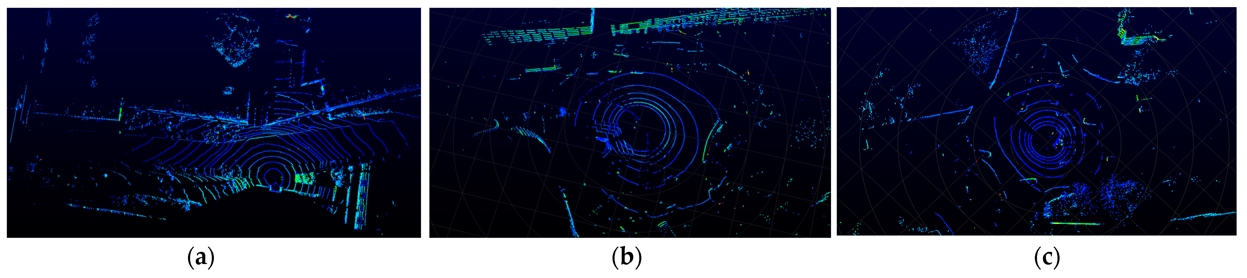
• For car, van, and pedestrian, the maximum tracking range at Site 1 is longer than that at Site 2 because a sensor with more laser beams is adopted at Site 1. For buses, the sensor can ‘see’ through a straight open road branch at Site 2, whereas at Site 1, bushes and trees occlude some of the beams when they attempt to spread further (seen as Figure 2). Therefore, buses can be tracked for longer at Site 2.

It can be concluded from the above observations that the size of objects and the number of laser beams matter greatly in the determination of maximum tracking range.

The algorithm proposed by Wu et al. [37] filters the background by dividing the space into grids with equal size and only considers points within 60 m; therefore, the maximum object detection range can only reach 60 m. Based on this background filtering algorithm, vehicles with a max distance of 29.1 m from the lidar sensor could be detected and tracked by Wu [10]. Another background construction algorithm has increased vehicle detection range to 100 m [33]. The above works are all based on a VLP-16 lidar sensor. In another proposed tracking-by-detection procedure [8], the tracking ranges with two different lidar sensors, RS-LiDAR-32 and VLP-16, are 45 m and 18 m, respectively. Compared with the above works, object tracking range using the proposed method has reached 111.3 m by RS-LiDAR-32 and 112.4 m by VLP-16. The above comparison is summarized in

Table 6. Comparison of developed method with other works in terms of Maximum Tracking Range.

Method	Sensor Type	Maximum Tracking Range (m)
[36]	VLP-16	60
[9]	VLP-16	29
[32]	VLP-16	100
[7]	VLP-16, RS-LiDAR-32	18, 45
Proposed method	VLP-16, RS-LiDAR-32	112, 111

.

5. Discussion

An advanced 3D object detection network, PV-RCNN, has been applied in this research. The performance of pedestrians was worse than vehicles according to the inference that the limited number of key points may harm the performance of objects with small sizes [34], which is also the reason why enlarging the number of training samples for the pedestrian class by adding KITTI data did not demonstrate any improvement. Vehicles were first detected by PV-RCNN, and later fine-grain classified into different categories using a RF classifier. This was undertaken with the consideration that discriminating vehicles from other objects first and further classifying them into different categories can usually provide better performance. It would be interesting to apply PV-RCNN as a multi-class detector when more training data is obtained. Further trials aim at adapting the network to make it directly operate on object proposals. PV-RCNN was operated using moving points, and it has also been tested with original lidar data to provide comprehensive comparisons.

There are three main sections in the proposed framework (as seen in Figure 1 in the manuscript): moving object segmentation, joint object detection and tracking, trajectory classification. Moving object segmentation is a pre-processing procedure which removes the irrelevant background and helps to reduce the number of false alarms. Object tracking and detection are performed in parallel, so tracking is not affected by detection, and therefore, the quality of trajectories is improved. As only representative clusters are used to identify the category of the trajectory from the detection results, the accuracy of trajectory classification is increased accordingly.

In the segmentation stage, empirical parameters include the minimum cluster size S₁, the maximum cluster size S₂, the minimum distance d between two clusters. Distance d between two vehicles would not vary greatly in different traffic situations. S₁ and S₂ are dependent on the sensor. Assuming the dataset covers all kinds of on-road objects, point density, which is affected by the type of sensor used, would be the only factor that influences the values of S₁ and S₂. It can be conducted statistically according to the dataset. In the object detection stage, there are no parameters that are dependent on the sensor. In the object tracking stage, parameter settings are shown in Table 1 of the manuscript. As can be seen from the table, only the assignment threshold is related to lidar sensor. In this study, it was set to 4 m considering both the maximum vehicle speed and lidar sensor frame rate. Given that the lidar frame rate is normally fixed at 10 Hz, the parameter does not need to change in a typical urban environment.

The input of the JDAT framework is original lidar data and the output are trajectories of vehicles and pedestrians. Detection and tracking are performed in parallel in the framework. In a similar work where joint object detection and tracking are also performed [38], the realization of parallelism relies on an object detection and a correlation network. The object correlation network is only part of the object tracking procedure, which means detection and tracking are not performed completely in parallel. Although object tracking in the JDAT framework is not based on advanced deep learning strategies, it is totally independent from object detection, which makes it more flexible and capable of generating higher quality outcomes such as trajectories with wider ranges and enhanced continuity.

The effectiveness of the proposed method has been assessed by both qualitative and quantitative analysis of various examples from different traffic scenes. Point cloud data has been processed to show the maximum tracking range of different object categories from two commonly used lidar sensors. Four widely existing on-road object categories, bus, car, van, and pedestrian, have been considered in the process. Other moving object categories in cities such as trucks, cyclists, and motorcyclists are not distinguished due to data limitations. Determining the maximum tracking ranges of these four categories provides installation guidance for real-world multi-lidar utilization.

6. Conclusions

A JDAT framework based on roadside lidar is proposed in this paper. Object detection and tracking are conducted in parallel when moving objects are segmented from the original point cloud by moving point detection and clustering. Trajectory classification is subsequently implemented to separate object trajectories into vehicles and pedestrians. Only dominant clusters regarded as representatives of each trajectory contribute to the classification procedure. Comprehensively evaluated by datasets from three study sites with two different lidar sensors, the presented framework shows potential to provide enhanced HRMTD by improving the quality of road user trajectories. The trajectory range has been extended by 22.5% based on object examples from different scenes; the continuity of the trajectories has been enhanced by bridging gaps arising from the absence of clusters. Moreover, the maximum effective tracking ranges of four different on-road object categories (bus, car, van, pedestrian), using the proposed methodology, have been evaluated. The research conducted thus far has some recognized limitations, primarily: trajectory discontinuity caused by persistent heavy occlusion could not be resolved as the proposed method can only optimize trajectories under partial occlusions; different weather conditions were not taken into account because all tests were conducted on days with fine weather; therefore, in future research, the utilization of multiple sensors is proposed to address issues related to heavy occlusions. It is also necessary to analyze the influence of different adverse weather conditions on effective tracking range to provide comprehensive quantitative information for practical application.

References

1. Fay, D.; Thakur, G.S.; Hui, P.; Helmy, A. Knowledge discovery and causality in urban city traffic: A study using planet scale vehicular imagery data. In Proceedings of the 6th ACM SIGSPATIAL International Workshop on Computational Transportation Science, Orlando, FL, USA, 5–8 November 2013. [Google Scholar]
2. Zhao, J.; Xu, H.; Liu, H.; Wu, J.; Zheng, Y.; Wu, D. Detection and tracking of pedestrians and vehicles using roadside LiDAR sensors. Transp. Res. Part C Emerg. Technol. 2019, 100, 68–87. [Google Scholar] [CrossRef]
3. Wu, J. Data processing algorithms and applications of LiDAR-enhanced connected infrastructure sensing. Ph.D. Thesis, University of Nevada, Reno, NV, USA, 2018. [Google Scholar]
4. Nagpure, A.K.; Gurjar, B.R.; Sahni, N.; Kumar, P. Pollutant emissions from road vehicle in mega city Kolkata, India: Past and present trends. Indian J. Air Pollut. Control 2010, 10, 18–30. [Google Scholar]
5. Xu, H.; Tian, Z.; Wu, J.; Liu, H.; Zhao, J. High-Resolution Micro Traffic Data from Roadside LiDAR Sensors for Connected-Vehicles and New Traffic Applications; University of Nevada, Solaris University Transportation Center: Reno, NV, USA, 2018. [Google Scholar]
6. Zhang, Z.; Zheng, J.; Xu, H.; Wang, X. Vehicle detection and tracking in complex traffic circumstances with roadside LiDAR. Transp. Res. Rec. 2019, 2673, 62–71. [Google Scholar] [CrossRef]
7. Zhao, J. Exploring the fundamentals of using infrastructure-based LiDAR sensors to develop connected intersections. Ph.D. Thesis, Texas Tech University, Lubbock, TX, USA, 2019. [Google Scholar]
8. Zhang, J.; Xiao, W.; Coifman, B.; Mills, J.P. Vehicle Tracking and Speed Estimation from Roadside Lidar. IEEE J. Sel. Top. Appl. Earth Obs. Remote Sens. 2020, 13, 5597–5608. [Google Scholar] [CrossRef]
9. Xiao, W.; Vallet, B.; Schindler, K.; Paparoditis, N. Simultaneous Detection and Tracking of Pedestrian from Velodyne Laser Scanning Data. ISPRS Ann. Photogramm. Remote Sens. Spat. Inf. Sci. 2016, 3, 295–302. [Google Scholar] [CrossRef] [Green Version]
10. Wu, J. An automatic procedure for vehicle tracking with a roadside LiDAR sensor. ITE J. Inst. Transp. Eng. 2018, 88, 32–37. [Google Scholar]
11. Chen, J.; Tian, S.; Xu, H.; Yue, R.; Sun, Y.; Cui, Y. Architecture of vehicle trajectories extraction with roadside LiDAR serving connected vehicles. IEEE Access 2019, 7, 100406–100415. [Google Scholar] [CrossRef]
12. Yan, Z.; Duckett, T.; Bellotto, N. Online learning for human classification in 3d lidar-based tracking. In Proceedings of the 2017 IEEE/RSJ International Conference on Intelligent Robots and Systems (IROS), Vancouver, BC, Canada, 24–28 September 2017. [Google Scholar]
13. Wu, J.; Xu, H.; Zheng, Y.; Zhang, Y.; Lv, B.; Tian, Z. Automatic vehicle classification using roadside LiDAR data. Transp. Res. Rec. 2019, 2673, 153–164. [Google Scholar] [CrossRef]
14. Zhang, J.; Pi, R.; Ma, X.; Wu, J.; Li, H.; Yang, Z. Object Classification with Roadside LiDAR Data Using a Probabilistic Neural Network. Electronics 2021, 10, 803. [Google Scholar] [CrossRef]
15. Wan, E.A.; Van Der Merwe, R. The Unscented Kalman Filter for Nonlinear Estimation. In Proceedings of the IEEE 2000 Adaptive Systems for Signal Processing, Communications, and Control Symposium, Lake Louise, AB, Canada, 4 October 2000. [Google Scholar]
16. Bar-Shalom, Y.; Daum, F.; Huang, J. The probabilistic data association filter. IEEE Control Syst. 2009, 29, 82–100. [Google Scholar]
17. Wu, J.; Zhang, Y.; Tian, Y.; Yue, R.; Zhang, H. Automatic Vehicle Tracking with LiDAR-Enhanced Roadside Infrastructure. J. Test Eval. 2020, 49, 121–133. [Google Scholar] [CrossRef]
18. Cui, Y.; Xu, H.; Wu, J.; Sun, Y.; Zhao, J. Automatic vehicle tracking with roadside LiDAR data for the connected-vehicles system. IEEE Intell. Syst. 2019, 34, 44–51. [Google Scholar] [CrossRef]
19. Weng, X.; Kitani, K. A baseline for 3d multi-object tracking. arXiv 2019, arXiv:1907.03961. [Google Scholar]
20. Weng, X.; Wang, J.; Held, D.; Kitani, K. 3d multi-object tracking: A baseline and new evaluation metrics. In Proceedings of the IEEE/RSJ International Conference on Intelligent Robots and Systems (IROS), Las Vegas, NV, USA, 24 October–24 January 2020. [Google Scholar]
21. Shi, S.; Wang, X.; Li, H. Pointrcnn: 3d object proposal generation and detection from point cloud. In Proceedings of the IEEE Conference on Computer Vision and Pattern Recognition, Long Beach, CA, USA, 15–20 June 2019. [Google Scholar]
22. Weng, X.; Kitani, K. Monocular 3d object detection with pseudo-lidar point cloud. In Proceedings of the IEEE/CVF International Conference on Computer Vision Workshops, Seoul, Korea, 27–28 October 2019. [Google Scholar]
23. Shi, S.; Guo, C.; Yang, J.; Li, H. PV-RCNN: The Top-Performing LiDAR-only Solutions for 3D Detection/3D Tracking/Domain Adaptation of Waymo Open Dataset Challenges. arXiv 2020, arXiv:2008.12599. [Google Scholar]
24. Geiger, A.; Lenz, P.; Stiller, C.; Urtasun, R. Vision meets robotics: The kitti dataset. Int. J. Rob. Res. 2013, 32, 1231–1237. [Google Scholar] [CrossRef] [Green Version]
25. Kuhn, H.W. The Hungarian method for the assignment problem. Nav. Res. Logist. Q. 1955, 2, 83–97. [Google Scholar] [CrossRef] [Green Version]
26. Wang, D.; Huang, C.; Wang, Y.; Deng, Y.; Li, H. A 3D Multiobject Tracking Algorithm of Point Cloud Based on Deep Learning. Math. Probl. Eng. 2020, 2020, 8895696. [Google Scholar] [CrossRef]
27. Weng, X.; Wang, Y.; Man, Y.; Kitani, K.M. Gnn3dmot: Graph neural network for 3d multi-object tracking with 2d-3d multi-feature learning. In Proceedings of the IEEE/CVF Conference on Computer Vision and Pattern Recognition, Seattle, WA, USA, 13–19 June 2020. [Google Scholar]
28. Tong, H.; Zhang, H.; Meng, H.; Wang, X. Multitarget Tracking Before Detection via Probability Hypothesis Density Filter. In Proceedings of the International Conference on Electrical and Control Engineering, Wuhan, China, 25–27 June 2010. [Google Scholar]
29. Ošep, A.; Mehner, W.; Voigtlaender, P.; Leibe, B. Track, then decide: Category-agnostic vision-based multi-object tracking. In Proceedings of the 2018 IEEE International Conference on Robotics and Automation (ICRA), Brisbane, QLD, Australia, 21–25 May 2018. [Google Scholar]
30. Mitzel, D.; Leibe, B. Taking Mobile Multi-Object Tracking to the Next Level: People, Unknown Objects, and Carried Items. In Proceedings of the European Conference on Computer Vision, Florence, Italy, 7–13 October 2012. [Google Scholar]
31. Gonzalez, H.; Rodriguez, S.; Elouardi. Track-Before-Detect Framework-Based Vehicle Monocular Vision Sensors. Sensors 2019, 19, 560. [Google Scholar] [CrossRef] [Green Version]
32. Chen, Q.A.; Tsukada, A. Detection-by-Tracking Boosted Online 3D Multi-Object Tracking. In Proceedings of the 2019 IEEE Intelligent Vehicles Symposium (IV), Paris, France, 9–12 June 2019. [Google Scholar]
33. Zhang, Z.; Zheng, J.; Xu, H.; Wang, X.; Fan, X.; Chen, R. Automatic background construction and object detection based on roadside LiDAR. IEEE Trans. Intell. Transp. Syst. 2019, 21, 4086–4097. [Google Scholar] [CrossRef]
34. Shi, S.; Guo, C.; Jiang, L.; Wang, Z.; Shi, J.; Wang, X.; Li, H. Pv-rcnn: Point-voxel feature set abstraction for 3d object detection. In Proceedings of the IEEE/CVF Conference on Computer Vision and Pattern Recognition, Seattle, WA, USA, 13–19 June 2020. [Google Scholar]
35. Syarif, I.; Prugel-Bennett, A.; Wills, G. SVM parameter optimization using grid search and genetic algorithm to improve classification performance. Telkomnika 2016, 14, 1502. [Google Scholar] [CrossRef]
36. SUPERVISELY. Available online: https://supervise.ly/ (accessed on 20 December 2021).
37. Wu, J.; Xu, H.; Sun, Y.; Zheng, J.; Yue, R. Automatic Background Filtering Method for Roadside LiDAR Data. Transp. Res. Rec. 2018, 2672, 106–114. [Google Scholar] [CrossRef]
38. Huang, K.; Hao, Q. Joint Multi-Object Detection and Tracking with Camera-LiDAR Fusion for Autonomous Driving. In Proceedings of the EEE/RSJ International Conference on Intelligent Robots and Systems (IROS), Prague, Czech Republic, 27 September–1 October 2021. [Google Scholar]
Figure 1. Flowchart of the proposed JDAT methodology.
Remotesensing 14 02124 g001
Figure 2. Three study sites used in this research: (a) Study Site 1: a single straight section of Claremont Road running through Newcastle University campus; (b) Study Site 2: a junction of the Great North Road and St Mary’s Place in Newcastle upon Tyne; (c) Study Site 3: a crossroad of Clayton Road and Osborne Road in the region of Jesmond, Newcastle upon Tyne.
Remotesensing 14 02124 g002
Figure 3. Classification performance with different n and p values. n is the number of representatives of a trajectory; p is the ratio of representatives identified as vehicles to n.
Remotesensing 14 02124 g003
Figure 4. PV-RCNN detection results at Study Site 1: (a) ground truth; (b) detection results.
Remotesensing 14 02124 g004
Figure 5. Trajectory classification results from Study Site 1. (a) Ground truth, (b) Trajectory classification results.
Remotesensing 14 02124 g005
Figure 6. The trajectories of nine vehicle examples from the two adopted methods: blue is from the tracking-by-detection method and red is from the proposed method.
Remotesensing 14 02124 g006aRemotesensing 14 02124 g006b
Figure 7. Vehicle examples demonstrating that JDAT can improve the continuity of vehicle trajectories.
Remotesensing 14 02124 g007aRemotesensing 14 02124 g007b