Superpixel Nonlocal Weighting Joint Sparse Representation for Hyperspectral Image Classification

Abstract

Joint sparse representation classification (JSRC) is a representative spectral–spatial classifier for hyperspectral images (HSIs). However, the JSRC is inappropriate for highly heterogeneous areas due to the spatial information being extracted from a fixed-sized neighborhood block, which is often unable to conform to the naturally irregular structure of land cover. To address this problem, a superpixel-based JSRC with nonlocal weighting, i.e., superpixel-based nonlocal weighted JSRC (SNLW-JSRC), is proposed in this paper. In SNLW-JSRC, the superpixel representation of an HSI is first constructed based on an entropy rate segmentation method. This strategy forms homogeneous neighborhoods with naturally irregular structures and alleviates the inclusion of pixels from different classes in the process of spatial information extraction. Afterwards, the superpixel-based nonlocal weighting (SNLW) scheme is built to weigh the superpixel based on its structural and spectral information. In this way, the weight of one specific neighboring pixel is determined by the local structural similarity between the neighboring pixel and the central test pixel. Then, the obtained local weights are used to generate the weighted mean data for each superpixel. Finally, JSRC is used to produce the superpixel-level classification. This speeds up the sparse representation and makes the spatial content more centralized and compact. To verify the proposed SNLW-JSRC method, we conducted experiments on four benchmark hyperspectral datasets, namely Indian Pines, Pavia University, Salinas, and DFC2013. The experimental results suggest that the SNLW-JSRC can achieve better classification results than the other four SRC-based algorithms and the classical support vector machine algorithm. Moreover, the SNLW-JSRC can also outperform the other SRC-based algorithms, even with a small number of training samples.

1. Introduction

Hyperspectral imaging collects the spectral response of the Earth’s surface from the visible to the infrared spectrum with a high spectral resolution, which enables the discrimination of different materials using the acquired rich spectral information. In particular, hyperspectral image (HSI) classification is used to assign a category label to each pixel for understanding the land cover and even its conditions. As a result, HSIs have been successfully applied in many application fields, such as urban planning [1], land use mapping [2], and natural resource monitoring [3].

In the past few decades, many approaches have been developed for the classification of HSIs, based mainly on the spectral information, such as the support vector machine (SVM) [4], multinomial logistic regression [5], and artificial neural network (ANN) [6], etc. However, noise is inevitably present in these methods, mainly due to the fact that they ignore the high spatial consistency of land cover [7]. Many attempts have been made recently to incorporate spatial information to promote the classification of HSIs [8,9,10,11,12,13,14,15,16,17,18,19]. Typical methods include the Gabor filter [9], extended random walker [10], morphological attribute profiles [11,12], edge preserving filters (EPF) [13,14,20], and the two-dimensional version of singular spectrum analysis (SSA) [15,16,19]. Moreover, to deal with the two typical problems of HSIs, i.e., the curse of dimensionality and small sample problems, a series of methods for dimensionality reduction and representation/useful feature learning have been developed [21,22,23,24,25]. These methods each have their own advantages.

More recently, researchers have introduced deep learning algorithms such as convolutional neural networks to HIS classification, which extract spatial information through local receptive fields [17,26]. Furthermore, several deeper networks and 2/3D CNN models have been investigated in HSI classification [18,27]. The deep learning-based classification methods have achieved superior classification accuracy, but they are usually time-consuming and require large amounts of training samples [28].

In recent years, sparse representation (SR) has attracted increasing attention in the field of face recognition [29] and signal processing [30,31], where a signal can be linearly represented or reconstructed by using a few determined elemental atoms in a low-dimensional subspace. By applying SR to HSI, sparsity can be adopted from the highly redundant spectral dimension for SR classification (SRC) of HSIs [32,33,34,35,36]. Due to the effect of noise, conventional pixelwise SRC has limitations when only spectral information is used for the classification of land cover. Therefore, joint sparse representation classification (JSRC) is proposed to combine both spatial and spectral information for more robust SRC in HSI [35]. JSRC performs classification by extending each pixel to a block of pixels centered at the given pixel, usually with a fixed size, and assuming that all pixels within the block belong to the same class. However, the fixed size of image blocks popularly adopted by JSRC-based methods is problematic, which has two main drawbacks. One is the inability to sufficiently exploit the structure diversity of land cover, and the other is the inclusion of noisy and heterogeneous pixels within the block, especially at the boundary of different classes.

Superpixel segmentation is a widely applied method for tackling the structure diversity of land cover, with typical segmentation methods including simple linear iterative clustering (SLIC) [37], graph-based image segmentation [38,39,40,41], and entropy rate superpixel (ERS) [42]. From the plentiful applications, it is concluded that SLIC focuses more on seeking the structural equilibrium of the segmented units [43]. Graph-based methods cannot accurately reflect the object boundary when the boundary is weak or with complex noise [39]. By contrast, ERS shows a better ability to delineate the boundary of targets. For the sparse-representation-based methods, Fang et al. [32] proposed a multiscale JSRC method with an adaptive sparsity strategy. It can achieve good performance only when proper scales are selected. Some researchers introduced superpixels to HSI classification, which are adaptively formed from over-segmented images for the effective description of land cover structures [33,44,45]. There is also a shape adaptive method [34] proposed to determine a polygon to represent spatial information, based on the similarity between the pixels in different directions and the center pixel. However, in practice, superpixels or adaptive shapes have to face internal heterogeneity and outliers [45] due to inherent noise in the image.

As the spatial information of fixed-sized blocks is degraded by heterogeneous and noisy pixels, some methods are employed to increase the contribution of the central pixel whilst decreasing the influence of noisy pixels in a block. For instance, Tu et al. [46] used correlation coefficients between the central pixel and samples to enhance classification decisions. A weighted joint nearest-neighbor method is applied to improve the reliability of the classification performance [47]. These methods, however, are highly dependent on the training samples. Additionally, a neighborhood weighting strategy is also used for the suppression of heterogeneous pixels within the fixed-sized block. For example, Qiao et al. [48] proposed a weighting scheme based on spectral similarity, where the weights are based on an implicit assumption that the center pixels of blocks are noise-free, which is hardly satisfied. Zhang et al. [49] proposed a nonlocal weighting scheme (NLW) based on the local self-similarity of images. NLW can preserve pixels with local self-similarity in a smooth region.

In summary, neither the adaptive neighborhood nor weighting-based methods can fully solve the aforementioned two drawbacks in JSRC, i.e., the structure diversity of land cover and noisy pixels. To this end, in this paper, we propose a superpixel-based nonlocal weighted JSRC (SNLW-JSRC) for HSI classification. By combining nonlocal weighting and the adaptive neighborhood together, the two drawbacks faced by JSRC can be solved simultaneously. Specifically, the superpixel-based weighting scheme (SNLW) is conducted to select pixels within superpixels according to their associated structural and spectral similarity measurements.

The major purposes of this paper can be concluded as follows:

(1)

To simultaneously and adaptively extract land cover structures while removing the effects of noise and outliers;

(2)

To fully explore the advantages of the superpixel and nonlocal weighting scheme for spectral–spatial feature extraction in HSI;

(3)

To outperform several classical SRC approaches and achieve improved data classification results of HSI.

The remainder of this paper is organized as follows. Section 2 introduces the traditional SRC and nonlocal weighted SRC. In Section 3, the detailed introduction of the proposed SNLW-JSRC is presented. The experimental results and analysis are given in Section 4. Finally, Section 5 provides some concluding remarks.

2. Nonlocal Weighted Sparse Representation for HSI Classification

For an HSI image, pixels from the same category lie in a low-dimensional subspace; thus, these pixels can be represented linearly by a small number of pixels from the same class [35]. This has formed the theoretical basis for SR classification (SRC) of HSI. Denote a pixel of HSI as a vector $x\in R^B$, where B is the number of spectral bands, and in total, the pixels are in C classes. We select $N_i$ training samples from the i-th class to form an overcomplete dictionary $D_i\in R^{B\times N_i}$, and the pixel $x$ of the i-th class can be reconstructed by [35]:

$$x=D_i\cdot a_i$$

(1)

where $a_i\in R^{N_i}$ represents the sparsity coefficient of $x$ with respect to $D_i$.

As the class of $x$ is unknown before classification, we need to build a dictionary $D$ that contains all the classes, i.e., $D=[D_1,D_2,\dots ,D_i,\dots ,D_C]\in R^{B\times N}$, where $N={\displaystyle \sum N_i}$, i = 1, 2,..., C. Accordingly, $x$ can be reconstructed by [35]:

$$x=D\cdot a$$

(2)

where $a=[a_1,a_2,\dots ,a_i,\dots ,a_C]\in R^N$ is the sparse coefficient of $x$ with respect to $D$. In order to obtain a sparse enough solution of $a$, we need to solve the following optimization problem [35]:

$$\begin{array}{l} \min {‖a‖}_0\\ s.t. x=D\cdot a\end{array}$$

(3)

where ${‖\cdot ‖}_0$ represents the number of non-zero elements of $a$. This is an NP-hard problem and can be solved by using the orthogonal matching pursuit (OMP) [50]. After determining $a$, the class of $x$ can be determined as follows [35]:

$$class\left(x\right)=\arg \min {‖x-D_i\cdot a_i‖}_F,i=1,2,\dots ,C$$

(4)

Since the SRC is based on the spectral characteristics of a single pixel, the spatial information of the pixel is ignored. As a result, it may lead to limited accuracy or sensitivity to noise [51]. To tackle this problem, joint sparse representation classification (JSRC) considering the spatial information of the pixel has been used to incorporate spectral–spatial information [35]. For a pixel $x$, its spatial neighborhood is denoted as $X\in R^{B\times K}$, where K denotes the number of pixels in $x$. The JSRC of $x$ in relation to $x$ can be derived as [47]:

$$X=D\cdot A$$

(5)

where $A=[A_1,A_2,\dots ,A_i,\dots ,A_C]\in R^{N\times K}$ represents the sparse coefficient of $X$ with respect to $D$, and $A_i\in R^{N_i\times K}$ denotes the sparse coefficient of $X$ with respect to $D_i$. Specifically, each column in $A$ shares the same sparse elements; hence, the spatial information of the land cover can be jointly utilized. In order to derive a solution of $A$, we need to solve the following objective function [47]:

$$\begin{array}{l} \min {‖A‖}_{row,0}\\ s.t. X=D\cdot A\end{array}$$

(6)

where ${‖\cdot ‖}_{row,0}$ represents the number of non-zero rows. Similarly, the optimization of Equation (6) is an NP-hard problem, which can be approximated by a variant of OMP called simultaneous OMP (SOMP) [52]. After obtaining $A$, the class of $x$ can be determined by [47]:

$$class\left(x\right)=\arg \min {‖x-D_i\cdot A_i‖}_F,i=1,2,\dots ,C$$

(7)

However, spectral–spatial information extracted by JSRC is easily affected by heterogeneous pixels in the defined neighborhood region $X$. In [49], a nonlocal weighting scheme (NLW) is developed to solve this problem. For a given test sample $x$, a fixed-sized block $X$ is obtained, centering on $x$. The weight of a neighboring pixel $y_i$ within $X$ is determined as follows [49]:

$${\omega }^{\prime }\left(x,y_i\right)=f\left(‖J\left(x\right)-J\left(y_i\right)‖\right),i=1,2,\dots ,T$$

(8)

where $J\left(\cdot \right)$ is a joint neighborhood definition function, and $J\left(x\right)$ and $J\left(y_i\right)$ refer to $x$-centric and $y_i$-centric HSI neighborhood blocks, respectively. $‖J\left(x\right)-J\left(y_i\right)‖$ represents the spectral–spatial difference between the two blocks, and T is the number of neighboring pixels. $f\left(\cdot \right)$ denotes a Tukey weight function [49] to weigh the spectral–spatial differences.

With the determined weights, a weighted region $X_W$ centered on $x$ can be obtained as below [49]:

$$\begin{array}{c}{X}_W={\omega }_X\cdot X\\ where {\omega }_X=\left[{\omega }^{\prime }\left(x,y_1\right),{\omega }^{\prime }\left(x,y_2\right),\dots ,{\omega }^{\prime }\left(x,y_{\mathrm{T}}\right)\right]\end{array}$$

(9)

where ${\omega }_X$ is a vector of the weights for neighboring pixels in $X$. Finally, JSRC is performed on $X_W$, using Equations (6) and (7) to obtain the labeled value of $x$. However, the weighted results of NLW cannot completely suppress the effects of noise and heterogeneous pixels, especially at the edges of land cover. Therefore, this paper proposes the SNLW scheme, which will be introduced in the following section.

3. The Proposed Superpixel-Based Nonlocal Weighted JSRC

3.1. Motivation

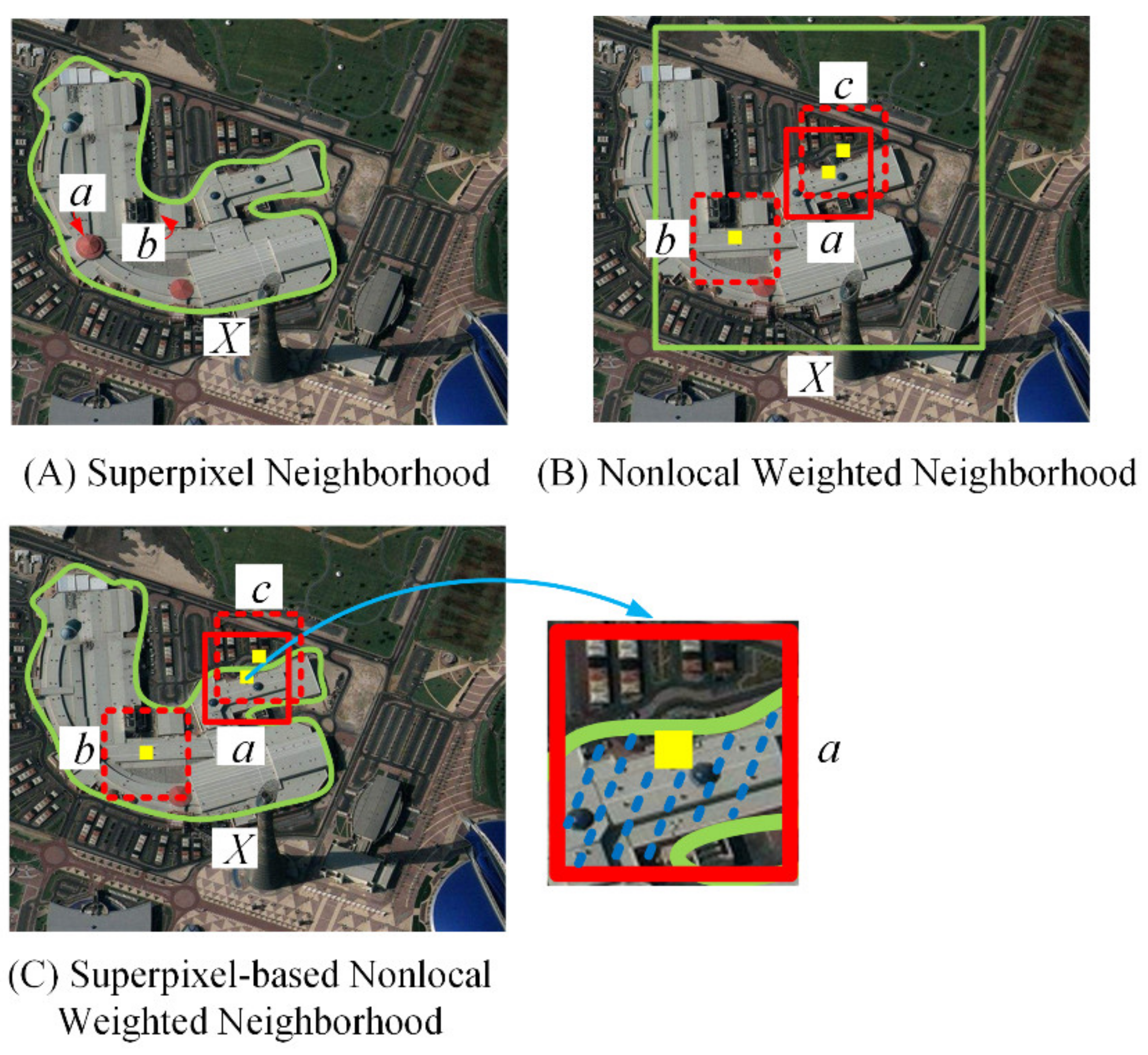
In addition to the NLW-based scheme, superpixel-based JSRC is another alternative for improving the accuracy. Figure 1 shows the different neighborhoods in JSRC.

As shown in Figure 1, they both have their own limitations. Figure 1A shows the superpixel neighborhood. As shown, a superpixel $X$ can give a good boundary partition of the building. However, there are still noisy pixels and outliers. For example, the red points a and b, which, respectively, represent red and black targets, are quite different from the building. Figure 1B shows the NLW-based weighting scheme, where $X$ is the defined neighborhood block for the central pixel a. Points b and c are two pixels within $X$. The red boxes denote the local structures for the three pixels, whose weights are calculated using Equation (10). Visually, pixels a and c have similar local structures (red boxes). Thus, the pixel c will be assigned a large weight to the test pixel a. This is clearly unreasonable since the pixel c itself is in a different class with respect to the test pixel a. In addition, although the pixel b is the same class as the test pixel a, its weight will be small because the local structures of a and b are quite different, as shown in Figure 1B. Obviously, the NLW neighborhood needs further improvement.

As for Figure 1C, it shows the proposed superpixel-based nonlocal weighting (SNLW) scheme. The superpixel is the neighborhood $X$ of the test pixel a, where $X$ includes pixel b but not pixel c. The red boxes also illustrate the local structures of the three pixels a, b and c. In the SNLW scheme, to eliminate the inclusion of pixels from different classes (such as pixel c), the local regions are further refined by the overlapped regions of $X$ and the red boxes, as illustrated in Figure 1C. As shown, the neighborhood is defined as the overlapping region filled with blue dashed lines in the close-up view for pixel a. Accordingly, the weights of pixels are calculated on these overlapping regions, which prevents the effects of external pixels. As a result, pixel b will be assigned a large weight with respect to test pixel a, and pixel c is naturally excluded. This illustrates how the proposed SNLW-JSRC works more effectively to make use of spectral–spatial information for improved HSI classification. The block diagram of the proposed approach is given in Figure 2, which is actually composed of three main steps, i.e., the generation of the superpixel, superpixel-based NLW, and JSRC for weighted mean superpixels. Details of these are presented in the next three subsections.

3.2. Generation of Superpixels

Superpixels can be formed by segmentation methods [42,43] for a single-band image. In the case of HSI, the conventional segmentation methods are not applicable since HSIs are three-dimensional tensor data. Therefore, it is generally necessary to perform dimensionality reduction. The commonly used dimensionality reduction methods include principal component analysis (PCA) [53], two-dimensional singular spectrum analysis (2D-SSA) [15], etc.; PCA is used in this paper for its efficiency. After applying PCA on HSI, the first PC is extracted, followed by the entropy rate segmentation (ERS) [42] to segment the image. The first PC is treated as a base map $G$, and the ERS method divides $G$ into $L$ closely connected pixel groups, namely superpixels. ERS first constructs an edge set of $E$ of $G$, which calculates the similarity between pairwise pixels. An edge subset $A\subseteq G$ is selected to construct the entropy rate $H\left(A\right)$ and balance the item $B\left(A\right)$. Finally, superpixel segmentation is obtained by solving the objective function below [42]:

$$\underset{A}{\max }\left\{H\left(A\right)+\lambda B\left(A\right)\right\} s.t. A\subseteq E$$

(10)

where $\lambda >0$ is a parameter to balance the contributions between $H\left(\cdot \right)$ and $B\left(\cdot \right)$.

3.3. Superpixel-Based Nonlocal Weighting Scheme (SNLW)

After deriving the superpixel map, the weighting process is implemented as follows. Figure 3 shows three local structures (a–c) in superpixels.

To identify the similarity between local structures—for example, as shown in Figure 3—the local structures in a (the green part) and b (the blue part) need be calculated first. We measure the spectral and structural information to jointly determine the similarity. However, when calculating the similarity between local structures, the local structures a and b are unequal in size. As seen in Figure 3C, our solution is to calculate the overlapping positions (the yellow part) of two local structures (a,b). Spectral information is obtained by the mean vector of local structures (a,b). Specifically, with a given scale s, the local structure $L\left(x\right)$ of the test pixel $x$ is extracted, and for another pixel $y$ in the superpixel, the local structure is $L\left(y\right)$, and the overlap position of $L\left(x\right)$ and $L\left(y\right)$ is $J\left(\cdot \right)$.

By evaluating the difference between the local structures, the weighting of $y$ can be decided by:

$$\begin{array}{c}{\omega }_{SP}^{\prime }\left(x,y\right)=f\left(\lambda ‖J\left(x\right)-J\left(y\right)‖+\left(1-\lambda ‖\overline{x}-\overline{y}‖\right)\right)\\ where \lambda =\frac{N_{J\left(x\right)}+N_{J\left(y\right)}}{N_{L\left(x\right)}+N_{L\left(y\right)}}\end{array}$$

(11)

where $\lambda$ is a weight item, and $N_{L\left(\cdot \right)}$ and $N_{J\left(\cdot \right)}$ are the pixel numbers of $L\left(\cdot \right)$ and $J\left(\cdot \right)$, respectively. $\overline{x}$ and $\overline{y}$ are the mean spectral information of all pixels in $L\left(x\right)$ and $L\left(y\right)$, respectively. $‖J\left(x\right)-J\left(y\right)‖$ and $‖\overline{x}-\overline{y}‖$ can be calculated by [49]:

$$‖J\left(x\right)-J\left(y\right)‖=\left|\frac{1}{B}{\displaystyle \sum _{k=1}^B\left(J_k\left(x\right)-J_k\left(y\right)\right)\otimes \mathsf{\Theta }}\right|$$

(12)

$$‖\overline{x}-\overline{y}‖=\frac{1}{B}\left(\frac{{\displaystyle {\sum }_{l=1}^{N_{L\left(x\right)}}{L}_{l,k}\left(x\right)}}{N_{L\left(x\right)}}-\frac{{\displaystyle {\sum }_{l=1}^{N_{L\left(y\right)}}{L}_{l,k}\left(y\right)}}{N_{L\left(y\right)}}\right)$$

(13)

where $J_k\left(\cdot \right)$ denotes the k-th band in $J\left(\cdot \right)$, $L_{l,k}\left(\cdot \right)$ denotes the k-th band and l-th pixel in $L\left(\cdot \right)$, B is the number of bands in the HSI, and $\otimes$ denotes the convolutional operator. $\mathsf{\Theta }$ is a Gaussian blur kernel, which measures the weights of the corresponding pixels within the patch of $J\left(x\right)-J\left(y\right)$. Note that the size of the Gaussian kernel is set to the size of the $J\left(\cdot \right)$.

In Equation (11), $f\left(\cdot \right)$ represents the weighting function; after the differences between pixels are calculated, the weights are defined as:

$$\begin{array}{c}{\omega }_{SP}^{\prime }\left(x,y\right)={\left(1-{\left(\frac{\lambda ‖J\left(x\right)-J\left(y\right)‖+\left(1-\lambda ‖\overline{x}-\overline{y}‖\right)}{\rho }\right)}^{\alpha }\right)}^2,\alpha \ge 1\\ where \rho =\max \left(‖\lambda J\left(x\right)-J\left(y\right)+‖\overline{x}-\overline{y}‖‖\right)\end{array}$$

(14)

Equation (14) is a monotonic descending function within [0, 1]; $\alpha$ controls the degree of compression. When $\alpha$ is relatively large, only those pixels with large differences are suppressed. $\rho$ represents the decay and is set to the maximum difference value within the superpixel, ensuring that the weighted results between two arbitrary pixels are the same. For a superpixel, a symmetric weighted matrix is obtained, as shown in Figure 2, in which each row represents a weighted result for a test pixel.

Furthermore, the weight matrix is processed as Equation (15) to better suppress heterogeneous pixels and better enhance similar pixels, in which:

$${\omega }_{SP}\left(x,y\right)=\left\{\begin{array}{c}0, 0\le {\omega }_{SP}^{\prime }\left(x,y\right)<OTSU\\ 1,OTSU\le {\omega }_{SP}^{\prime }\left(x,y\right)<1\end{array}\right.$$

(15)

where OTSU is a threshold adaptively acquired by the Otsu threshold method [54], which decides whether the corresponding pixel will be adopted or discarded.

3.4. JSRC for Weighted Mean Superpixels

In order to speed up the sparse representation and eliminate the effect of noisy pixels, we propose to centralize the information of similar pixels, i.e., weighted mean, in our superpixel-based SR. For a given superpixel $X_{SP}=\left[x_1,x_2,\dots ,x_S\right]\in R^{B\times S}$, $S$ is the number of superpixels, and $x_i$ is the i-th pixel within $X_{SP}$. The weights of $x_i$ are defined as ${\omega }_{SP}\left(x_i\right)={\left[{\omega }_{SP}\left(x_i,y_1\right),{\omega }_{SP}\left(x_i,y_2\right),\dots ,{\omega }_{SP}\left(x_i,y_S\right)\right]}^T$. The weighted mean pixel $x_{wsp}^i$ of $x_i$ can be determined according to the weights by:

$$x_{wsp}^i=\frac{{\displaystyle \sum {\omega }_{SP}\left(x_i\right)\cdot X_{SP}{}^T}}{{\displaystyle \sum {\omega }_{SP}\left(x_i\right)}}$$

(16)

The weighted mean of the superpixel, $X_{WSP}$, is the collection of $x_{wsp}^i$, i.e., $X_{WSP}=\left[x_{wsp}^i,x_{wsp}^2,\dots ,x_{wsp}^S\right]$. Finally, we assume all pixels within a superpixel from the same class and apply JSRC for classification, using Equations (6) and (7) to obtain the label.

4. Experimental Results and Discussion

In the experimental part, the performance of the proposed SNLW-JSRC approach is evaluated using four publicly available HSI datasets: Indian Pines, Pavia University (PaviaU), Salinas, and 2013 GRSS Data Fusion Contest (DFC2013) [55]. The proposed method was benchmarked with several classical HSI classification approaches, including pixel-wise sparse representation classification (SRC) [29], joint sparse representation classification (JSRC) [35], nonlocal weighted joint sparse representation (NLW-JSRC) [49], superpixel-based joint sparse representation (SP-JSRC), its single-scale version in [33], and SVM [4]. In these methods, SRC and SVM are typical pixel-wise classifiers; others are spectral–spatial-based classifiers. The NLW-JSRC method uses the same weighting scheme as ours, yet it is based on local self-similarity, i.e., spectral–spatial information. The SP-JSRC is a superpixel-level spectral–spatial classifier. The quantitative metrics used in this study include the overall accuracy (OA), the average accuracy (AA), and the Kappa coefficient (Kappa) [32].

4.1. Datasets

The Indian Pines dataset was acquired by the Airborne Visible/Infrared Imaging Spectrometer (AVIRIS) sensor in Northwestern Indiana, USA. The spectral range is from 400 to 2450 nm. We removed 20 water absorption bands and used the remaining 200 bands for experiments. The imaged scene had 145 × 145 pixels with a 20 m spatial resolution, among which 10,249 pixels are labeled. The total number of classes in this dataset is 16.

The PaviaU dataset was acquired in Pavia University, Italy, by the Reflective Optics System Imaging Spectrometer. The spatial resolution of the dataset is 1.3 m, while the spectral range is from 430 nm to 860 nm. After removing 12 water absorption bands, we keep 103 bands from the original 115 bands for the experiment. The imaged scene has 610 × 340 pixels, among which 42,776 pixels are labeled. The number of classes is 9.

The Salinas scene dataset was also collected by the AVIRIS sensor in Salinas Valley, California, which has a continuous spectral coverage from 400 nm to 2450 nm. The spatial resolution of the dataset is 3.7 m. There are 512 × 217 pixels, among which 54,129 pixels were labeled and used for the experiment. After removing the water absorption bands, we keep the remaining 204 bands in the experiments. The number of classes is 16.

The DFC2013 dataset is a part of the outcome of the 2013 GRSS Data Fusion Contest, and it was acquired by the NSF-funded Center for Airborne Laser Mapping over the University of Houston campus and its neighboring area in the summer of 2012. This dataset has 144 bands in the 380–1050 nm spectral region. The spatial resolution of the dataset is 2.5 m. There are 349 × 1905 pixels, and 15029 of them were labeled as training and testing pixels. The number of classes is 15.

4.2. Comparison of Classification Results

For SVM, we use the RBF kernel, where a fivefold cross-validation is used. The parameters of SRC were tuned to the best. For all the SRC-based methods, the sparse level was set to 3, as used in [18]. Additionally, the scale of local blocks is 5 × 5 for JSRC and 11 × 11 for NLW-JSRC. For SP-JSRC and SNLW-JSRC, the size of superpixels was chosen from a sequence, which is 400, 500, 600, 700, 800, 900, 1000, 1100, and 1200, and we chose 500 for Indian Pines, 1100 for PaviaU, 400 for Salinas, and 1000 for DFC2013. The parameter α in Equation (14) is set to 3 in this paper.

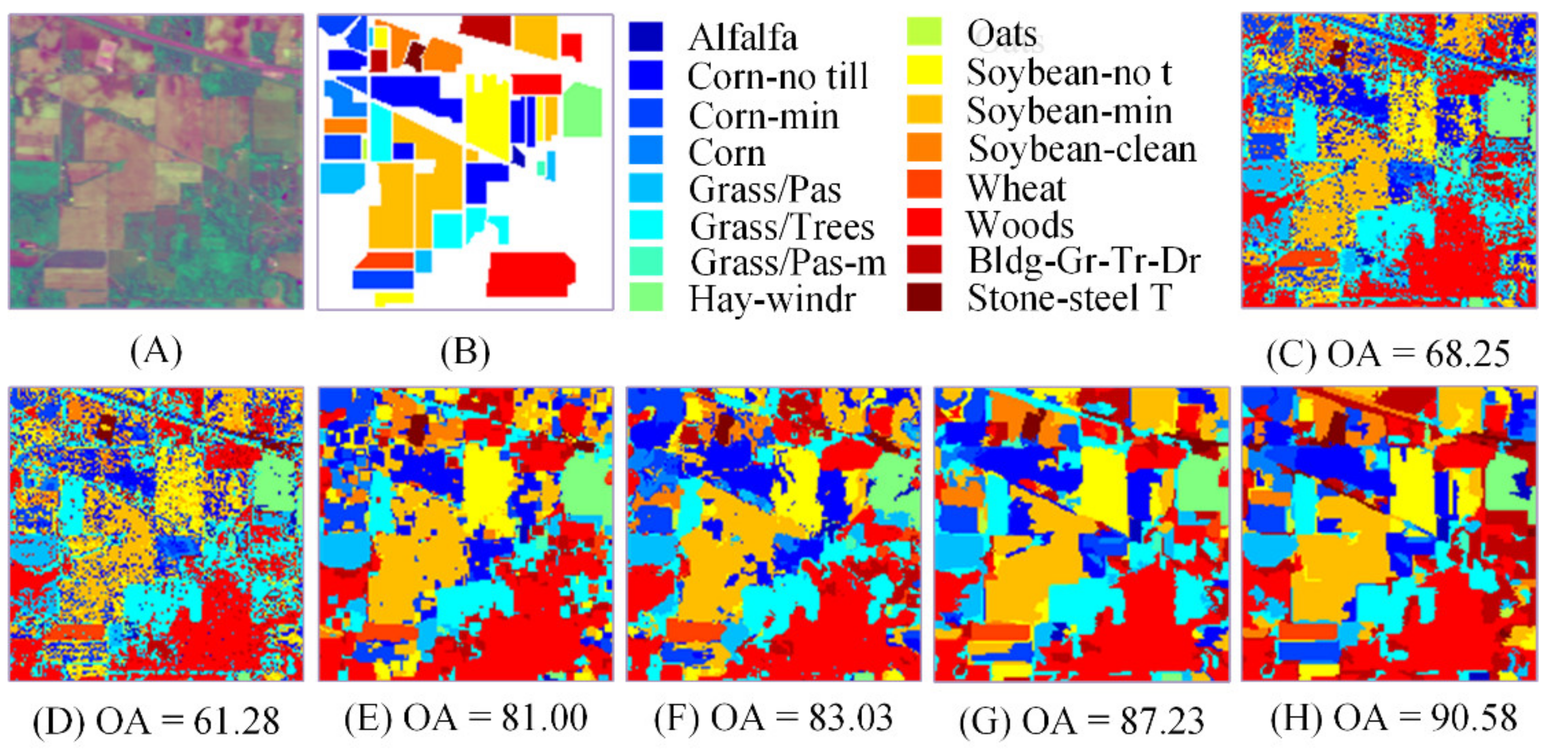
The first experiment was on the Indian Pines, where 2.5% of samples in each class were randomly selected for training, and the remaining (97.5%) for testing. The specific numbers of training and testing samples for each class are summarized in

Table 1. Class-based numbers of training and testing samples for Indian Pines.

Class	Name	Training	Testing
1	Alfalfa	2	48
2	Corn-no till	38	1462
3	Corn-mintill	22	850
4	Corn	7	242
5	Grass-pasture	13	494
6	Grass-trees	20	747
7	Grass-pasture-mowed	1	29
8	Hay-windrowed	13	489
9	Oats	1	20
10	Soybean-notill	26	994
11	Soybean-mintill	65	2513
12	Soybean-clean	16	606
13	Wheat	6	209
14	Woods	34	1294
15	Bldg-grass-trees-drives	11	394
16	Stone-steel-towers	3	94
Total		278	10,485

. The quantitative results for our approach and the benchmarking ones are given in

Table 2. Accuracy of Indian Pines classification results (the best result in each row is highlighted in bold).

Class	SVM	SRC	JSRC	NLW-JSRC	SP-JSRC	SNLW-JSRC
1	43.18	40.23	68.41	45.91	97.95	98.01
2	59.55	44.89	69.83	72.22	81.33	82.96
3	53.03	38.45	71.09	74.67	84.18	82.35
4	16.45	26.45	54.68	62.51	60.95	63.91
5	84.47	70.57	86.81	83.55	85.57	84.73
6	91.42	89.21	94.61	93.77	97.37	97.13
7	74.07	60.37	75.56	52.96	96.30	96.30
8	96.57	92.45	96.72	96.31	99.81	96.38
9	10.53	26.32	51.05	41.58	100.00	100.00
10	64.41	56.02	81.61	80.96	90.06	93.81
11	70.71	66.14	86.4	88.57	90.12	92.10
12	52.25	27.58	54.62	61.98	79.20	88.26
13	85.93	86.98	91.46	92.42	99.55	99.56
14	88.56	87.34	96.24	96.76	98.91	96.13
15	21.01	24.12	48.70	51.84	53.03	75.53
16	78.89	86.56	91.44	84.23	90.67	90.56
OA(%)	68.61	61.33	80.67	82.09	87.81	89.60
AA(%)	61.94	57.73	76.20	73.77	87.81	89.86
Kappa	0.64	0.56	0.78	0.79	0.86	0.88

for comparison, where the best results are highlighted in bold. Note that to reduce the impact of randomness, all the experiments were repeated for 10 runs, where the averaged results are reported. Figure 4 shows the classification maps of the last run.

According to the visualization results of Figure 4, the classification map of pixel-wise SRC has serious noise, while the classification results based on the spectral–spatial information classifier are obviously superior in both quantitative and qualitative terms. Although the classification result of JSRC suppresses the influence of noise, there is obvious misclassification. For NLW-JSRC, partial misclassification of JSRC is solved, but because NLW-JSRC cannot make good use of spectral–spatial information in the weighting process, the improvement is limited. In SP-JSRC, due to the use of superpixels, good boundaries of the classification map and higher accuracy were obtained, but the noise and outliers within several superpixels brought misclassifications. For the SNLW-JSRC, the quantitative result in Table 2 is the best among the comparison methods. In terms of qualitative results, the classification map is almost immune to noise, has good boundaries, and overcomes the problem of superpixel internal noise.

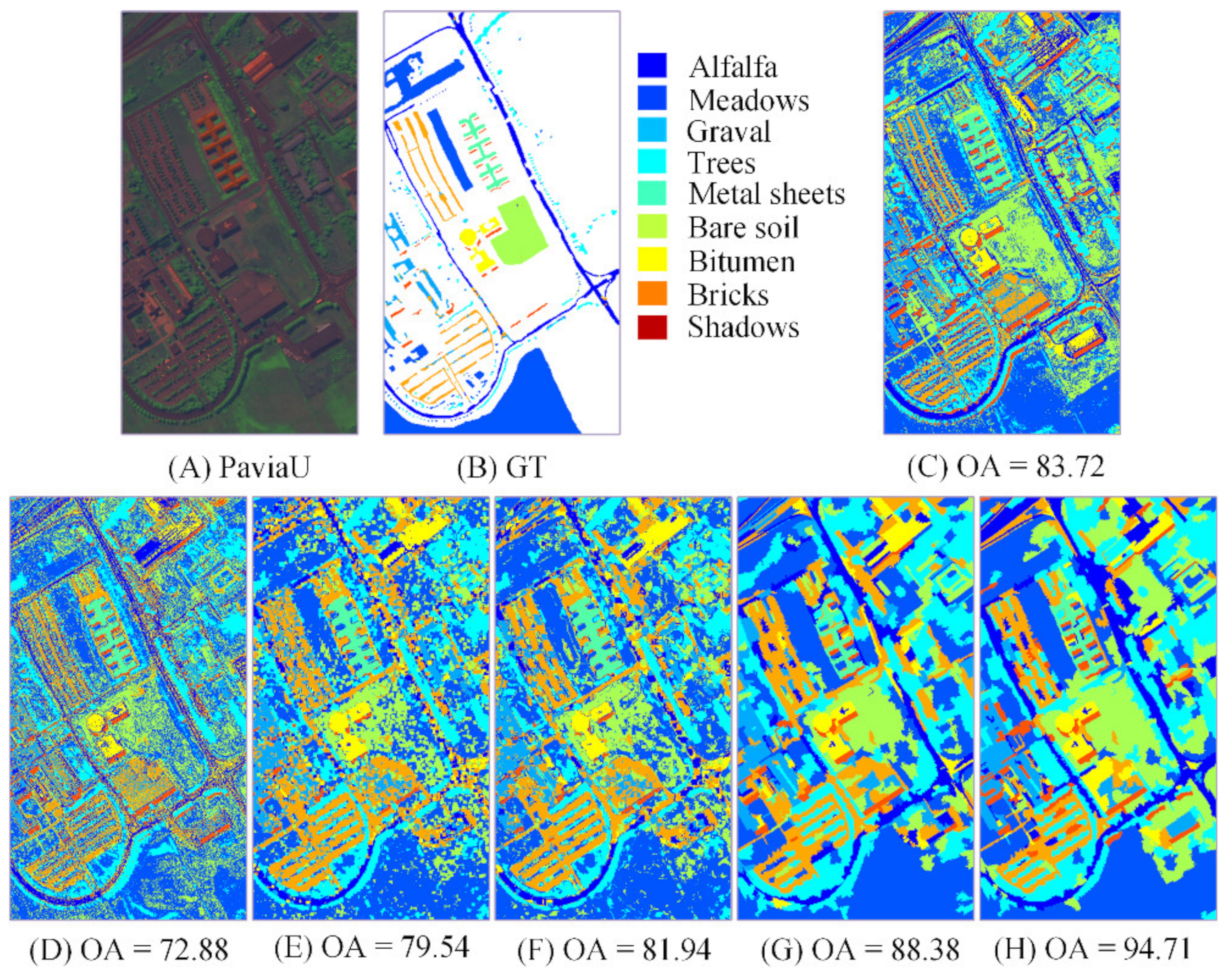
The second experiment was conducted on the PaviaU dataset. For each class of this dataset, 50 samples were randomly selected as training samples, and the rest of the samples were taken as testing samples. The specific numbers of training and testing samples are shown in

Table 3. Class-based numbers of training and testing samples for PaviaU.

Class	Name	Training	Testing
1	Alfalfa	50	6881
2	Meadows	50	18,899
3	Graval	50	2349
4	Trees	50	3314
5	Metal sheets	50	1595
6	Bare soil	50	5279
7	Bitumen	50	1580
8	Bricks	50	3932
9	Shadows	50	1107
Total		450	44,936

. The quantitative results for comparison methods and the proposed method are tabulated in

Table 4. Accuracy of PaviaU classification results (the best result in each row is highlighted in bold).

Class	SVM	SRC	JSRC	NLW-JSRC	SP-JSRC	SNLW-JSRC
1	76.02	57.02	46.69	51.54	65.58	82.90
2	84.16	71.23	85.62	87.95	89.43	94.46
3	89.56	67.44	88.09	88.07	95.48	97.33
4	87.23	89.01	92.84	93.09	83.38	81.47
5	98.84	99.40	99.52	99.68	94.32	98.30
6	83.37	62.10	78.03	80.28	93.37	96.93
7	93.75	85.45	98.35	97.28	100.00	100.00
8	75.66	67.35	83.43	85.45	93.23	96.26
9	100.00	96.06	68.75	61.40	85.03	95.89
OA(%)	83.63	70.51	79.57	81.62	86.75	92.64
AA(%)	87.62	77.23	82.37	82.75	88.87	93.73
Kappa	0.79	0.62	0.74	0.76	0.83	0.90

, in which the best results are in bold. As with Indian Pines, all the results were averaged in 10 runs with different training sets. The obtained estimation maps of the last run are given in Figure 5.

As shown in Figure 5, compared to pixel-wise classifiers and block-based classifiers, superpixel-based methods achieve better noise suppression and boundary division. However, the superpixel information used by the SP-JSRC method may contain noise and outliers, thus causing misclassifications in the superpixel level. In SNLW-JSRC, these misclassifications were well solved due to the SNLW strategy. The quantitative results listed in Table 4 also confirm the superiority of SNLW-JSRC. In addition, the advantages of SNLW-JSRC on PaviaU are more obvious than those on Indian Pines. This may be because of the higher spatial resolution of the PaviaU dataset.

For the experiment of Salinas, we randomly selected 0.25% of the samples in each category as training samples, and the rest (99.75%) were taken as testing samples. The specific numbers of training and testing samples for each class are available in

Table 5. Class-based numbers of training and testing samples for Salinas.

Class	Name	Training	Testing
1	Weeds_1	6	2003
2	Weeds_2	10	3716
3	Fallow	5	1971
4	Fallow plow	4	1390
5	Fallow smooth	7	2671
6	Stubble	10	3949
7	Celery	9	3570
8	Grapes	29	11,242
9	Soil	16	6187
10	Corn	9	3269
11	Lettuce 4 wk	3	1065
12	Lettuce 5 wk	5	1922
13	Lettuce 6 wk	3	913
14	Lettuce 7 wk	3	1067
15	Vinyard untrained	19	7249
16	Vinyard trellis	5	1802
Total		143	53,986

. The quantitative and qualitative results for comparison methods and the proposed method are tabulated in

Table 6. Accuracy of Salinas classification results (the best result in each row is highlighted in bold).

Class	SVM	SRC	JSRC	NLW-JSRC	SP-JSRC	SNLW-JSRC
1	98.60	97.37	99.83	99.91	100.00	100.00
2	99.25	97.67	99.74	99.72	99.53	99.42
3	82.29	76.29	84.32	83.91	89.49	80.55
4	98.13	98.91	88.05	95.99	96.13	99.93
5	96.18	96.44	93.38	99.23	99.29	99.26
6	96.35	99.42	99.71	99.99	99.79	99.67
7	99.44	98.98	99.17	99.82	99.73	99.05
8	72.37	66.05	76.84	75.00	86.27	91.23
9	98.84	97.08	99.92	99.97	99.86	99.41
10	85.56	79.49	90.81	93.67	95.74	88.18
11	88.17	92.14	96.42	99.56	98.54	98.37
12	97.97	93.95	86.20	97.98	100.00	100.00
13	97.81	95.90	93.92	98.74	97.82	97.91
14	91.28	85.64	92.25	97.96	95.14	90.95
15	56.09	56.78	70.94	69.38	80.85	91.80
16	95.12	74.03	94.98	94.01	97.01	91.34
OA(%)	85.37	82.52	88.42	89.19	93.45	94.88
AA(%)	90.84	87.89	91.66	94.05	95.95	95.44
Kappa	0.84	0.81	0.87	0.88	0.93	0.94

and Figure 6, respectively. In Table 6, the best results of each row are in bold. The results shown in Table 6 were also averaged in 10 runs with different training sets, and the classification map was obtained from the last run.

As shown in Figure 6, all the four SRC variants integrated with spatial information have less salt and pepper noise compared to the spectral-reliant SVM and SRC. Moreover, the misclassification of the proposed SNLW-JSRC is the lowest. This is also confirmed by the quantitative results tabulated in Table 6. In addition, it is shown that although the SNLW-JSRC still produced the best OA and Kappa, its advantages on the Salinas dataset are not so remarkable as on the PaviaU dataset. This comes from the simple scene and lower spatial resolution of Salinas, which make its spatial heterogeneity lower. From Table 6, we can see that the performance of SP-JSRC and SNLW-JSRC is similar. This also indicates that SNLW-JSRC has a better effect on the HSI with higher heterogeneity.

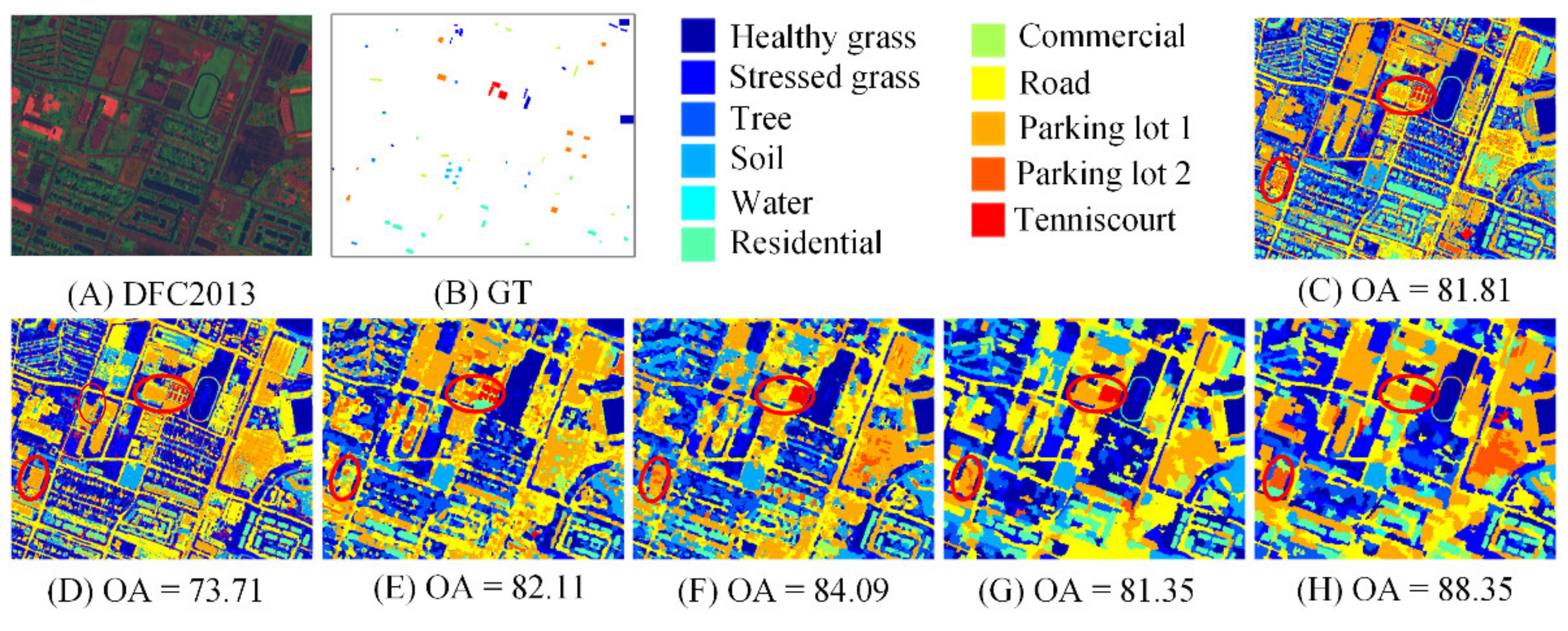
The last experiment was conducted on the DFC2013 dataset. In this paper, a central part of the Houston University campus containing 336 × 420 pixels belonging to 11 classes of targets is selected as the experimental area. For each class of this dataset, we selected 1% of samples as training samples, and the rest (99%) were taken as testing samples. The specific numbers of training and testing samples for each class are shown in

Table 7. Class-based numbers of training and testing samples for DFC2013.

Class	Name	Training	Testing
1	Healthy grass	5	454
2	Stressed grass	3	211
3	Tree	2	137
4	Soil	2	153
5	Water	1	6
6	Residential	4	372
7	Commercial	1	54
8	Road	3	275
9	Parking lot 1	5	483
10	Parking lot 2	1	8
11	Tennis court	3	247
Total		30	2400

. The quantitative and qualitative results for comparison methods and the proposed method are tabulated in

Table 8. Accuracy of DFC2013 classification results (the best result in each row is highlighted in bold).

Class	SVM	SRC	JSRC	NLW-JSRC	SP-JSRC	SNLW-JSRC
1	99.31	93.52	99.22	99.49	100	99.33
2	89.18	96.25	80.48	90.48	58.8	86.49
3	92.81	62.44	83.41	83.7	72.96	70.74
4	88.28	99.01	99.8	98.41	99.21	89.67
5	100	100	78	0	80	100
6	92.69	71.25	76.52	77.17	76.14	88.45
7	30.57	35.66	37.36	40.38	33.96	33.58
8	62.43	56.14	70.99	76.43	78.49	90.77
9	53.95	62.47	72.2	71.28	78.16	74.25
10	21.43	18.57	94.29	92.86	57.14	100
11	89.59	83.24	92.42	94.39	91.07	100
OA(%)	80.17	75.77	82.35	83.85	81.65	86.83
AA(%)	74.57	70.78	80.43	74.96	75.08	84.84
Kappa	0.77	0.72	0.79	0.81	0.79	0.85

and Figure 7, respectively. The results shown in Table 8 were also averaged in 10 runs with different training sets, in which the best results are in bold. The classification map displayed in Figure 7 was obtained from the last run.

From Table 8, we can conclude that for the more complicated DFC2013 dataset, the SNLW-JSRC performs with obvious superiority, with OA and Kappa equal to 86.83% and 0.85, respectively. Similar to the PaviaU dataset, the spatial resolution and heterogeneity of DFC2013 are higher; this also reveals that the SNLW-JSRC can not only provide adaptive neighborhood information following the irregular morphological characteristics of targets but also eliminates the outliers and noise in the neighborhood. Especially for the targets with confusing spectral characteristics, such as soil, residential areas, and parking lot areas, the SNLW-JSRC shows better classification performance, as highlighted in Figure 7C–H by the red circles.

To further test the computational efficiency of the proposed SNLW-JSRC, we calculated the running time of each experiment. These experiments were conducted on a PC with an Intel (R) Pentium (R) CPU 2.9 GHz and 6 GB RAM, and Matlab R2017b. The CPU times (in seconds) of the compared methods are listed in

Table 9. CPU times of compared methods.

Methods	Indian Pines (s)	PaviaU (s)	Salinas (s)	DFC2013 (s)
SVM	7	31	13	10
SRC	12	40	38	3
JSRC	44	75	65	23
NLW-JSRC	248	532	467	39
SP-JSRC	6	13	26	2
SNLW-JSRC	18	146	173	26

.

As shown, due to the first four algorithms paying more and more attention to the use of spatial neighboring information, their CPU time increases. By contrast, the CPU time of SP-JSRC is much lower since it performs superpixel-level sparse decomposition. Compared to the SP-JSRC, the proposed SNLW-JSRC adds a more time-consuming SNLW-based weighting procedure. Thus, the SNLW-JSRC consumes more computing time than the SP-JSRC. Nevertheless, the SNLW-JSRC is clearly more efficient than the NLW-JSRC. Overall, comprehensively considering its superior classification performance and efficiency, the proposed SNLW-JSRC is a more preferable algorithm. Even so, mixed programming with C language and Matlab, as well as the use of GPU, will further speed up the calculation process, and SNLW-JSRC is still optional.

4.3. Effect of Superpixel Numbers

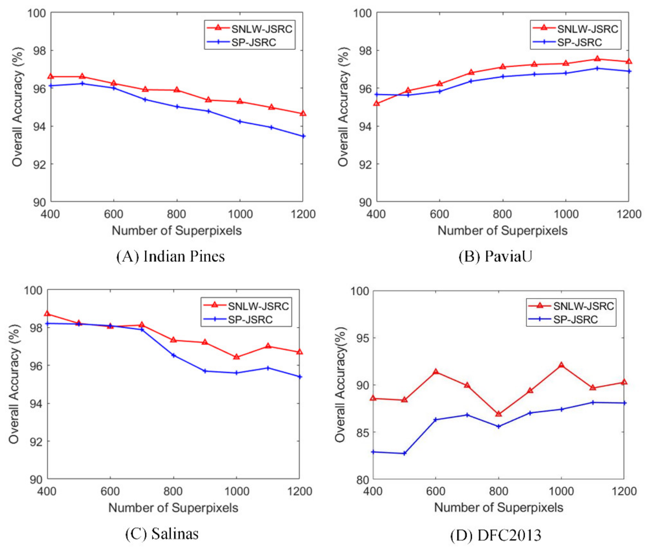
The number of superpixels affects the size of the superpixel. Generally, the larger the superpixel number, the smaller the superpixel size, and vice versa. Therefore, the number of superpixels has a great influence on the quality of superpixel segmentation. Here, we set up a sequence of superpixel numbers—400, 500, 600, 700, 800, 900, 1000, 1100, and 1200—to explore the impact on SNLW-JSRC and SP-JSRC. In the experiment, the number of training samples was 10%, 200, 1%, and 2% of each class for Indian Pines, PaviaU, Salinas, and DFC2013, respectively. The remaining parameters were the same as those in Section 4.2. The effect of the superpixel number on the Indian Pines, PaviaU Salinas, and DFC 2013 datasets is shown in Figure 8. As can be observed, for almost all the numbers of superpixels, SNLW-JSRC has an obvious improvement over SP-JSRC due to better noise suppression achieved by SNLW-JSRC. In addition, after an upward trend of accuracy, a downward trend is presented. As the number of superpixels becomes larger and larger, the superpixel scale becomes smaller and smaller, resulting in failure to provide sufficient spatial information for proper classification. However, the decline in the accuracy of SNLW-JSRC is slower than that of SP-JSRC, indicating that noise suppression promotes the robustness of classification.

4.4. Effect of the Number of Training Samples

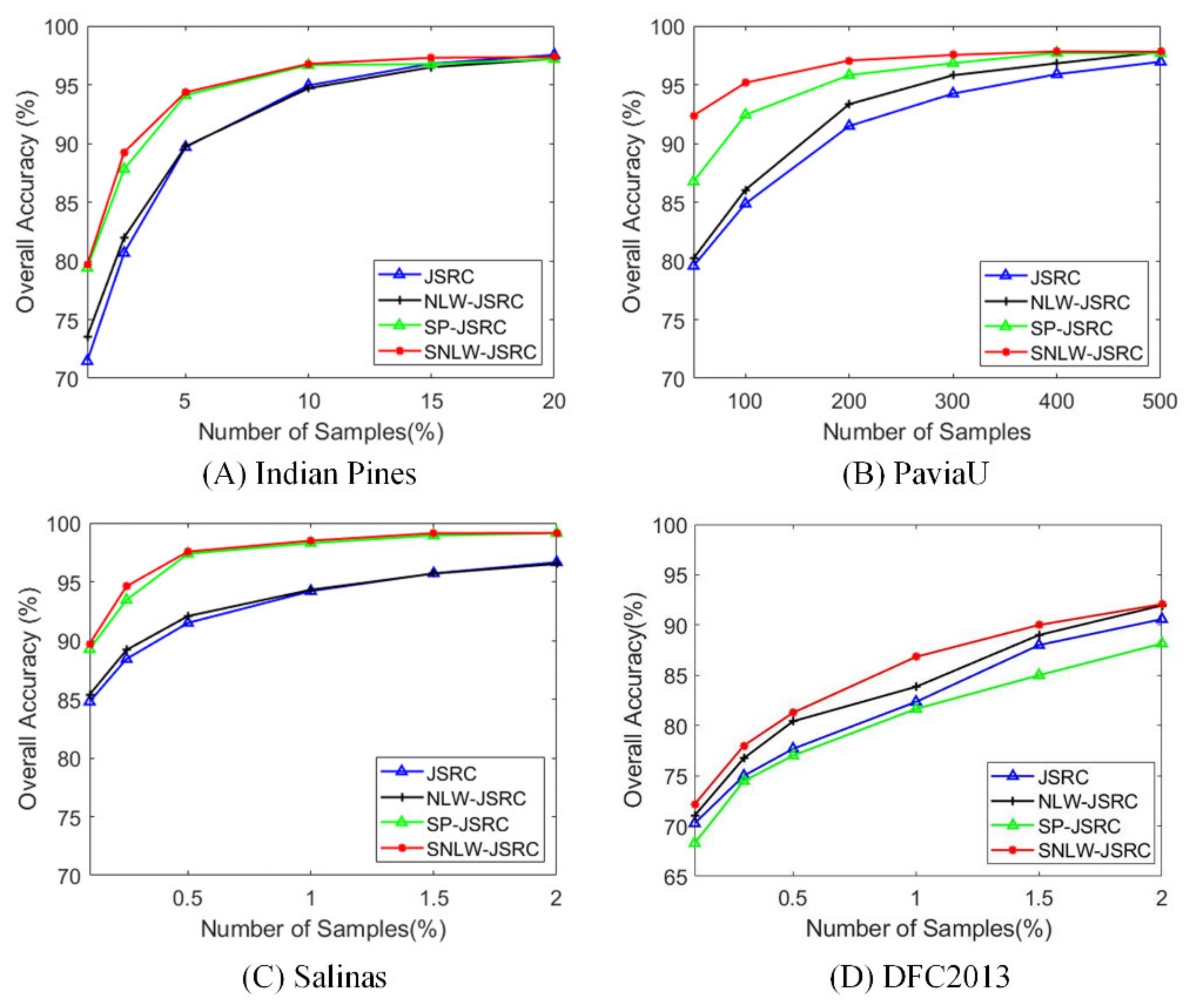
Here, we explore the impact of the number of training samples on different methods, including JSRC, NLW-JSRC, SP-JSRC, and SNLW-JSRC, on four datasets. We set the percentage of training samples as 1%, 2.5%, 5%, 10%, 15%, and 20% of each class for Indian Pines, select 50, 100, 200, 300, 400, and 500 samples of each class for PaiviaU, and set the percentage as 0.1%, 0.25%, 0.5%, 1%, 1.5%, and 2% of each class for Salinas and DFC2013. The remaining parameters are the same as those in Section 4.2. The results are shown in Figure 9. The overall trend is that the more training samples included, the higher the classification accuracy of each method. When the sample percentage is 10% for Indian Pines, 200 for PaviaU, 1% for Salinas, and 2% for DFC 2013, the growth trend becomes slower. In particular, SNLW-JSRC is basically superior to other methods, especially for the more complex PaviaU data, indicating that the proposed method is good at handling complex data. When the training sample is small, SNLW-JSRC can achieve a better improvement since SNLW-JSRC achieves good noise suppression and makes the classification more robust to samples.

5. Conclusions

In this paper, we proposed superpixel-based nonlocal weighting joint sparse representation classification (SNLW-JSRC) for hyperspectral image classification. Firstly, superpixels help to obtain a relatively spectral-consistent neighborhood. The nonlocal weighting is used to further purify the spatial neighborhood, and finally, JSRC enables superpixel-level classification. The results on four benchmark datasets show that the proposed method is superior to the comparative methods in terms of improved classification accuracy, comparable computing time, and robustness to small numbers of training samples. The analysis of the classification results also shows that the proposed method can simultaneously solve the two problems of block neighborhoods in JSRC, which not only provides adaptive neighborhood information but also eliminates the outliers and noise in the neighborhood. However, the results of this paper are still limited by the results of segmented superpixels; thus, serious over-segmentation will also lead to a lack of spatial information. This will form the basis of our future investigation.

References

1. Abbate, G.; Fiumi, L.; Lorenzo, C.D.; Vintila, R. Evaluation of remote sensing data for urban planning. Applicative examples by means of multispectral and hyperspectral data. In Proceedings of the 2003 2nd GRSS/ISPRS Joint Workshop on Remote Sensing and Data Fusion over Urban Areas, Berlin, Germany, 22–23 May 2003; pp. 201–205. [Google Scholar]
2. Jouan, A.; Allard, Y. Land use mapping with evidential fusion of features extracted from polarimetric synthetic aperture radar and hyperspectral imagery. Inf. Fusion 2004, 5, 251–267. [Google Scholar] [CrossRef]
3. Papeş, M.; Tupayachi, R.; Martínez, P.; Peterson, A.T.; Powell, G.V.N. Using hyperspectral satellite imagery for regional inventories: A test with tropical emergent trees in the Amazon Basin. J. Veg. Sci. 2010, 21, 342–354. [Google Scholar] [CrossRef]
4. Melgani, F.; Bruzzone, L. Support vector machines for classification of hyperspectral remote-sensing images. In Proceedings of the IEEE International Geoscience and Remote Sensing Symposium, Toronto, ON, Canada, 24–28 June 2002; Volume 501, pp. 506–508. [Google Scholar]
5. Jiao, H.; Zhong, Y.; Zhang, L. Artificial DNA computing-based spectral encoding and matching algorithm for hyperspectral remote sensing data. IEEE Trans. Geosci. Remote Sens. 2012, 50, 4085–4104. [Google Scholar] [CrossRef]
6. Marpu, P.R.; Gamba, P.; Niemeyer, I. Hyperspectral data classification using an ensemble of class-dependent neural networks. In Proceedings of the 2009 First Workshop on Hyperspectral Image and Signal Processing: Evolution in Remote Sensing, Grenoble, France, 26–28 August 2009; pp. 1–4. [Google Scholar]
7. Liu, X.; Bourennane, S.; Fossati, C. Reduction of signal-dependent noise from hyperspectral images for target detection. IEEE Trans. Geosci. Remote Sens. 2014, 52, 5396–5411. [Google Scholar] [CrossRef]
8. Sun, X.; Zhou, F.; Dong, J.; Gao, F.; Mu, Q.; Wang, X. Encoding spectral and spatial context information for hyperspectral image classification. IEEE Geosci. Remote Sens. Lett. 2017, 14, 2250–2254. [Google Scholar] [CrossRef]
9. Jia, S.; Shen, L.; Li, Q. Gabor Feature-based collaborative representation for hyperspectral imagery classification. IEEE Trans. Geosci. Remote Sens. 2015, 53, 1118–1129. [Google Scholar] [CrossRef]
10. Sun, B.; Kang, X.; Shutao, L.; Benediktsson, J.A. Random-walker-based collaborative learning for hyperspectral image classification. IEEE Trans. Geosci. Remote Sens. 2017, 55, 212–222. [Google Scholar] [CrossRef]
11. Fauvel, M.; Benediktsson, J.A.; Chanussot, J.; Sveinsson, J.R. Spectral and spatial classification of hyperspectral data using SVMs and morphological profiles. IEEE Trans. Geosci. Remote Sens. 2008, 46, 3804–3814. [Google Scholar] [CrossRef] [Green Version]
12. Mura, M.D.; Villa, A.; Benediktsson, J.A.; Chanussot, J.; Bruzzone, L. Classification of hyperspectral images by using extended morphological attribute profiles and independent component analysis. IEEE Geosci. Remote Sens. Lett. 2011, 8, 542–546. [Google Scholar] [CrossRef] [Green Version]
13. Kotwal, K.; Chaudhuri, S. Visualization of hyperspectral images using bilateral filtering. IEEE Trans. Geosci. Remote Sens. 2010, 48, 2308–2316. [Google Scholar] [CrossRef] [Green Version]
14. Peng, H.; Rao, R. Hyperspectral image enhancement with vector bilateral filtering. In Proceedings of the 2009 16th IEEE International Conference on Image Processing (ICIP), Cairo, Egypt, 7–10 November 2009; pp. 3713–3716. [Google Scholar]
15. Zabalza, J.; Ren, J.; Zheng, J.; Han, J.; Zhao, H.; Li, S.; Marshall, S. Novel two-dimensional singular spectrum analysis for effective feature extraction and data classification in hyperspectral imaging. IEEE Trans. Geosci. Remote Sens. 2015, 53, 4418–4433. [Google Scholar] [CrossRef] [Green Version]
16. Fu, H.; Sun, G.; Zabalza, J.; Zhang, A.; Ren, J.; Jia, X. A novel spectral-spatial singular spectrum analysis technique for near real-time in situ feature extraction in hyperspectral imaging. IEEE J. Sel. Top. Appl. Earth Obs. Remote Sens. 2020, 13, 2214–2225. [Google Scholar] [CrossRef]
17. Yu, S.; Jia, S.; Xu, C. Convolutional neural networks for hyperspectral image classification. Neurocomputing 2017, 219, 88–98. [Google Scholar] [CrossRef]
18. Sun, G.; Zhang, X.; Jia, X.; Ren, J.; Zhang, A.; Yao, Y.; Zhao, H. Deep fusion of localized spectral features and multi-scale spatial features for effective classification of hyperspectral images. Int. J. Appl. Earth Obs. Geoinf. 2020, 91, 102157. [Google Scholar] [CrossRef]
19. Sun, G.; Fu, H.; Ren, J.; Zhang, A.; Zabalza, J.; Jia, X.; Zhao, H. SpaSSA: Superpixelwise adaptive ssa for unsupervised spatial-spectral feature extraction in hyperspectral image. IEEE Trans. Cybern. 2021, 1–12. [Google Scholar] [CrossRef]
20. Kang, X.; Li, S.; Benediktsson, J.A. Spectral–spatial hyperspectral image classification with edge-preserving filtering. IEEE Trans. Geosci. Remote Sens. 2014, 52, 2666–2677. [Google Scholar] [CrossRef]
21. Huang, H.; Yang, M. Dimensionality reduction of hyperspectral images with sparse discriminant embedding. IEEE Trans. Geosci. Remote Sens. 2015, 53, 5160–5169. [Google Scholar] [CrossRef]
22. Tschannerl, J.; Ren, J.; Yuen, P.; Sun, G.; Zhao, H.; Yang, Z.; Wang, Z.; Marshall, S. MIMR-DGSA: Unsupervised hyperspectral band selection based on information theory and a modified discrete gravitational search algorithm. Inf. Fusion 2019, 51, 189–200. [Google Scholar] [CrossRef] [Green Version]
23. Mou, L.; Saha, S.; Hua, Y.; Bovolo, F.; Bruzzone, L.; Zhu, X.X. Deep Reinforcement learning for band selection in hyperspectral image classification. IEEE Trans. Geosci. Remote Sens. 2022, 60, 5504414. [Google Scholar] [CrossRef]
24. Ma, K.Y.; Chang, C.I. Iterative training sampling coupled with active learning for semisupervised spectral–spatial hyperspectral image classification. IEEE Trans. Geosci. Remote Sens. 2021, 59, 8672–8692. [Google Scholar] [CrossRef]
25. Luo, F.; Zou, Z.; Liu, J.; Lin, Z. Dimensionality reduction and classification of hyperspectral image via multistructure unified discriminative embedding. IEEE Trans. Geosci. Remote Sens. 2022, 60, 1–16. [Google Scholar] [CrossRef]
26. Li, S.; Song, W.; Fang, L.; Chen, Y.; Ghamisi, P.; Benediktsson, J.A. Deep learning for hyperspectral image classification: An overview. IEEE Trans. Geosci. Remote Sens. 2019, 57, 6690–6709. [Google Scholar] [CrossRef] [Green Version]
27. Paoletti, M.E.; Haut, J.M.; Fernandez-Beltran, R.; Plaza, J.; Plaza, A.J.; Pla, F. Deep pyramidal residual networks for spectral–spatial hyperspectral image classification. IEEE Trans. Geosci. Remote Sens. 2019, 57, 740–754. [Google Scholar] [CrossRef]
28. Huang, H.; Sun, G.; Zhang, X.; Hao, Y.; Zhang, A.; Ren, J.; Ma, H. Combined multiscale segmentation convolutional neural network for rapid damage mapping from postearthquake very high-resolution images. J. Appl. Remote Sens. 2019, 13, 022007. [Google Scholar] [CrossRef]
29. Yang, M. Face recognition via sparse representation. In Wiley Encyclopedia of Electrical and Electronics Engineering; John Wiley & Sons, Inc.: Hoboken, NJ, USA, 1999; pp. 1–12. [Google Scholar] [CrossRef]
30. Cho, N.; Kuo, C.J. Sparse representation of musical signals using source-specific dictionaries. IEEE Signal Process. Lett. 2010, 17, 913–916. [Google Scholar] [CrossRef]
31. Bruckstein, A.M.; Donoho, D.L.; Elad, M. From sparse solutions of systems of equations to sparse modeling of signals and images. SIAM Rev. 2009, 51, 34–81. [Google Scholar] [CrossRef] [Green Version]
32. Fang, L.; Li, S.; Kang, X.; Benediktsson, J.A. spectral–spatial hyperspectral image classification via multiscale adaptive sparse representation. IEEE Trans. Geosci. Remote Sens. 2014, 52, 7738–7749. [Google Scholar] [CrossRef]
33. Zhang, S.; Li, S. Spectral-spatial classification of hyperspectral images via multiscale superpixels based sparse representation. In Proceedings of the 2016 IEEE International Geoscience and Remote Sensing Symposium (IGARSS), Beijing, China, 10–15 July 2016; pp. 2423–2426. [Google Scholar]
34. Fu, W.; Li, S.; Fang, L.; Kang, X.; Benediktsson, J.A. Hyperspectral image classification via shape-adaptive joint sparse representation. IEEE J. Sel. Top. Appl. Earth Obs. Remote Sens. 2016, 9, 556–567. [Google Scholar] [CrossRef]
35. Chen, Y.; Nasrabadi, N.M.; Tran, T.D. Hyperspectral image classification using dictionary-based sparse representation. IEEE Trans. Geosci. Remote Sens. 2011, 49, 3973–3985. [Google Scholar] [CrossRef]
36. Luo, F.; Zhang, L.; Zhou, X.; Guo, T.; Cheng, Y.; Yin, T. Sparse-adaptive hypergraph discriminant analysis for hyperspectral image classification. IEEE Geosci. Remote Sens. Lett. 2020, 17, 1082–1086. [Google Scholar] [CrossRef]
37. Achanta, R.; Shaji, A.; Smith, K.; Lucchi, A.; Fua, P.; Süsstrunk, S. SLIC superpixels compared to state-of-the-art superpixel methods. IEEE Trans. Pattern Anal. Mach. Intell. 2012, 34, 2274–2282. [Google Scholar] [CrossRef] [PubMed] [Green Version]
38. Felzenszwalb, P.F.; Huttenlocher, D.P. Efficient graph-based image segmentation. Int. J. Comput. Vis. 2004, 59, 167–181. [Google Scholar] [CrossRef]
39. Sellars, P.; Aviles-Rivero, A.I.; Schönlieb, C. Superpixel contracted graph-based learning for hyperspectral image classification. IEEE Trans. Geosci. Remote Sens. 2020, 58, 4180–4193. [Google Scholar] [CrossRef] [Green Version]
40. Saha, S.; Mou, L.; Zhu, X.X.; Bovolo, F.; Bruzzone, L. Semisupervised change detection using graph convolutional network. IEEE Geosci. Remote Sens. Lett. 2021, 18, 607–611. [Google Scholar] [CrossRef]
41. Wan, S.; Gong, C.; Zhong, P.; Du, B.; Zhang, L.; Yang, J. Multiscale dynamic graph convolutional network for hyperspectral image classification. IEEE Trans. Geosci. Remote Sens. 2020, 58, 3162–3177. [Google Scholar] [CrossRef] [Green Version]
42. Liu, M.; Tuzel, O.; Ramalingam, S.; Chellappa, R. Entropy rate superpixel segmentation. In Proceedings of the CVPR 2011, Colorado Springs, CO, USA, 20–25 June 2011; pp. 2097–2104. [Google Scholar]
43. Psalta, A.; Karathanassi, V.; Kolokoussis, P. Modified versions of SLIC algorithm for generating superpixels in hyperspectral images. In Proceedings of the 2016 8th Workshop on Hyperspectral Image and Signal Processing: Evolution in Remote Sensing (WHISPERS), Los Angeles, CA, USA, 21–24 August 2016; pp. 1–5. [Google Scholar]
44. Roscher, R.; Waske, B. Superpixel-based classification of hyperspectral data using sparse representation and conditional random fields. In Proceedings of the 2014 IEEE Geoscience and Remote Sensing Symposium, Quebec City, QC, Canada, 13–18 July 2014; pp. 3674–3677. [Google Scholar]
45. Tong, F.; Tong, H.; Jiang, J.; Zhang, Y. Multiscale union regions adaptive sparse representation for hyperspectral image classification. Remote Sens. 2017, 9, 872. [Google Scholar] [CrossRef] [Green Version]
46. Tu, B.; Zhang, X.; Kang, X.; Zhang, G.; Wang, J.; Wu, J. Hyperspectral image classification via fusing correlation coefficient and joint sparse representation. IEEE Geosci. Remote Sens. Lett. 2018, 15, 340–344. [Google Scholar] [CrossRef]
47. Tu, B.; Huang, S.; Fang, L.; Zhang, G.; Wang, J.; Zheng, B. Hyperspectral image classification via weighted joint nearest neighbor and sparse representation. IEEE J. Sel. Top. Appl. Earth Obs. Remote Sens. 2018, 11, 4063–4075. [Google Scholar] [CrossRef]
48. Qiao, T.; Yang, Z.; Ren, J.; Yuen, P.; Zhao, H.; Sun, G.; Marshall, S.; Benediktsson, J.A. Joint bilateral filtering and spectral similarity-based sparse representation: A generic framework for effective feature extraction and data classification in hyperspectral imaging. Pattern Recognit. 2018, 77, 316–328. [Google Scholar] [CrossRef] [Green Version]
49. Zhang, H.; Li, J.; Huang, Y.; Zhang, L. A nonlocal weighted joint sparse representation classification method for hyperspectral imagery. IEEE J. Sel. Top. Appl. Earth Obs. Remote Sens. 2014, 7, 2056–2065. [Google Scholar] [CrossRef]
50. Li, J.; Wu, Z.; Feng, H.; Wang, Q.; Liu, Y. Greedy orthogonal matching pursuit algorithm for sparse signal recovery in compressive sensing. In Proceedings of the 2014 IEEE International Instrumentation and Measurement Technology Conference (I2MTC) Proceedings, Montevideo, Uruguay, 12–15 May 2014; pp. 1355–1358. [Google Scholar]
51. Liu, Y.; Liu, S.; Wang, Z. A general framework for image fusion based on multi-scale transform and sparse representation. Inf. Fusion 2015, 24, 147–164. [Google Scholar] [CrossRef]
52. Tropp, J.A. Algorithms for simultaneous sparse approximation. Part II: Convex relaxation. Signal Process. 2006, 86, 589–602. [Google Scholar] [CrossRef]
53. Zabalza, J.; Ren, J.; Ren, J.; Liu, Z.; Marshall, S. Structured covariance principal component analysis for real-time onsite feature extraction and dimensionality reduction in hyperspectral imaging. Appl. Opt. 2014, 53, 4440–4449. [Google Scholar] [CrossRef] [Green Version]
54. Merzban, M.H.; Elbayoumi, M. Efficient solution of Otsu multilevel image thresholding: A comparative study. Expert Syst. Appl. 2019, 116, 299–309. [Google Scholar] [CrossRef]
55. Debes, C.; Merentitis, A.; Heremans, R.; Hahn, J.; Frangiadakis, N.; Van Kasteren, T.; Liao, W.; Bellens, R.; Pižurica, A.; Gautama, S.; et al. Hyperspectral and LiDAR Data Fusion: Outcome of the 2013 GRSS Data Fusion Contest. IEEE J. Sel. Top. Appl. Earth Obs. Remote Sens. 2014, 7, 2405–2418. [Google Scholar] [CrossRef]
Figure 1. The illustration of different neighborhoods in JSRC: (A) superpixel neighborhood, (B) nonlocal weighted neighborhood, and (C) superpixel-based nonlocal weighted neighborhood. Three points ac are pixels; a is a testing pixel, and b and c are neighboring pixels. X is the neighborhood of pixel a, and it is a superpixel in (A,C) and a square block in (B).
Remotesensing 14 02125 g001
Figure 2. The workflow of the proposed SNLW-JSRC.
Remotesensing 14 02125 g002
Figure 3. The local structures in superpixels: (A,B) are two local structure samples, in which green and blue pixels represent the local structures, and (C) denotes the calculation position (yellow pixels) of structures a and b.
Remotesensing 14 02125 g003
Figure 4. Indian Pines image: (A) composite color image and (B) ground truth; estimation map obtained by (C) SVM; (D) SRC; (E) JSRC; (F) NLW-JSRC; (G) SP-JSRC; (H) SNLW-JSRC.
Remotesensing 14 02125 g004
Figure 5. PaviaU image: (A) composite color image and (B) ground truth; estimation map obtained by (C) SVM; (D) SRC; (E) JSRC; (F) NLW-JSRC; (G) SP-JSRC; (H) SNLW-JSRC.
Remotesensing 14 02125 g005
Figure 6. Salinas image: (A) composite color image and (B) ground truth; estimation map obtained by (C) SVM; (D) SRC; (E) JSRC; (F) NLW-JSRC; (G) SP-JSRC; (H) SNLW-JSRC.
Remotesensing 14 02125 g006
Figure 7. DFC2013 image: (A) composite color image and (B) ground truth; estimation map obtained by (C) SVM; (D) SRC; (E) JSRC; (F) NLW-JSRC; (G) SP-JSRC; (H) SNLW-JSRC.
Remotesensing 14 02125 g007
Figure 8. Effects of the superpixel number on four datasets; (AD) are based on Indian Pines, PaviaU, Salinas, and DFC2013 images, respectively.
Remotesensing 14 02125 g008
Figure 9. Effects of the number of training samples; (AD) are based on Indian Pines, PaviaU, Salinas, and DFC2013 images, respectively.
Remotesensing 14 02125 g009