Article

Optimum Feature and Classifier Selection for Accurate Urban Land Use/Cover Mapping from Very High Resolution Satellite Imagery

1
Department of Geography, Kharazmi University, Tehran 1417466191, Iran
2
Centre Eau Terre Environnement, Institute National de la Recherche Scientifique (INRS), Quebec City, QC G1K 9A9, Canada
3
School of Surveying and Geospatial Engineering, College of Engineering, University of Tehran, Tehran 1417466191, Iran
4
Canada Centre for Mapping and Earth Observation, Natural Resources Canada, Ottawa, ON K1S 5K2, Canada
*
Author to whom correspondence should be addressed.
Remote Sens. 2022, 14(9), 2097; https://doi.org/10.3390/rs14092097
Submission received: 9 March 2022 / Revised: 24 April 2022 / Accepted: 24 April 2022 / Published: 27 April 2022
(This article belongs to the Special Issue Optical Remote Sensing Applications in Urban Areas II)

Abstract

:
Feature selection to reduce redundancies for efficient classification is necessary but usually time consuming and challenging. This paper proposed a comprehensive analysis for optimum feature selection and the most efficient classifier for accurate urban area mapping. To this end, 136 multiscale textural features alongside a panchromatic band were initially extracted from WorldView-2, GeoEye-3, and QuickBird satellite images. The wrapper-based and filter-based feature selection were implemented to optimally select the best ten percent of the primary features from the initial feature set. Then, machine leaning algorithms such as artificial neural network (ANN), support vector machine (SVM), and random forest (RF) classifiers were utilized to evaluate the efficiency of these selected features and select the most efficient classifier. The achieved optimum feature set was validated using two other images of WorldView-3 and Pleiades. The experiments revealed that RF, particle swarm optimization (PSO), and neighborhood component analysis (NCA) resulted in the most efficient classifier and wrapper-based and filter-based methods, respectively. While ANN and SVM’s process time depended on the number of input features, RF was significantly resistant to the criterion. Dissimilarity, contrast, and correlation features played the greatest contributing role in the classification performance among the textural features used in this study. These trials showed that the feature number could be reduced optimally to 14 from 137; these optimally selected features, alongside the RF classifier, can produce an F1-measure of about 0.90 for different images from five very high resolution satellite sensors for various urban geographical landscapes. These results successfully achieve our goal of assisting users by eliminating the task of optimal feature selection and classifier, thereby increasing the efficiency of urban land use/cover classification from very high resolution images. This optimal feature selection can also significantly reduce the high computational load of the feature-engineering phase in the machine and deep learning approaches.

1. Introduction

Higher spatial resolution increases intraclass variances, resulting in high interclass spectral confusion in satellite image classification [1]. The issue is naturally associated with the sensor resolution, and it cannot be addressed by increasing the number of spectral bands to enhance the superclass abilities. Thus, an alternative can be the use of spatial information such as textural features [2]. Statistical approaches based on the gray-level co-occurrence matrix (GLCM) were reported as the most beneficial textural analysis [3,4] among four main types of procedures for textual analysis recognized by [5]. This information is helpful for various applications, such as distinguishing crops [6,7] and classifying tree species [8,9,10] and urban mapping [4,11,12,13,14]. However, using high-dimensional spatial feature sets can result in redundancy among the features; overfitting of the classifiers [15,16,17,18]; building complex models; making model interpretation challenging; and requiring additional computational time, storage, and processing compared to a more optimal input dataset [19,20].
As a solution to the issues mentioned above, researchers have paid lots of attention to feature selection (FS) as an approach to selecting the most relevant features for predefined classes [21,22]. The FS methods are categorized into three categories, including filter, wrapper, and hybrid algorithms. Filter approaches utilize statistical properties independent of the classification performance to eliminate less-significant input in feature sets [23,24,25]. They are computationally inexpensive and fast [26,27]. On the other hand, wrapper methods consider the relation between learning algorithms and training data [28,29]. This is why they outperform filter models in terms of accuracy [30,31,32]. However, they are slower and computationally more expensive [27,30]. The hybrid method uses two algorithms by various evaluation standards in the different search stages [26]. Naeini, et al. [33] investigated several wrapper-based algorithms, such as particle swarm optimization (PSO), genetic algorithm (GA), artificial bee colony (ABC), and honey-bee mating (HBM), to select the best spectral and textural parameters for very high spatial resolution data classification. Then, the selected features were input to various classifiers resulting in better performance for the PSO-selected feature dataset. Hamedianfar, et al. [34] carried out feature selection through consolidation of PSO and artificial neural network (ANN) applied to WorldView-2 data for land use/cover mapping with extreme gradient boosting (XGBoost). They reached an overall accuracy of above 89%. Concerning the filter models surveys, Wu, et al. [35] conducted comparative analyses on four filter-based FS methods, including maximal–minimal associated index (MMAI), maximum relevance minimum redundancy (MRMR), relief-F, and correlation-based FS (CFS). They applied these methods to hyperspectral band selection and showed that MMAI led to the best performance. In another comparative analysis, Malan, et al. [36] showed that neighborhood component analysis (NCA) outperformed GA, principal component analysis (PCA), and relief-F in terms of the kappa coefficient for signal analysis. Ren, et al. [37] implemented an improved version of the relief-F method called partitioned relief-F and compared it with PCA and the original relief-F via classification outputs. The experiments showed a slight increase of up to 4% for the improved method compared to the classical ones. Despite the merits of FS methods, they are intensive because no self-evident and consistent guidelines have been suggested for this process yet.
The non-parametric machine learning methods such as artificial neural networks (ANNs), support vector machine (SVM), and random forest (RF) have significantly captured remote sensing experts’ attention in the classification of heterogeneous surfaces and big data analysis throughout the recent decades [38,39,40]. These algorithms were developed for land use/cover mapping [41,42,43] and were compared based on their classification performance by Rogan, et al. [44] and Camargo, et al. [45]. Concerning these surveys, Xie, et al. [39] exploited vegetation indices and textural and topographical data from bi-temporal ZiYuan-3 multispectral and stereo images to detect tree, forest, and land use classes. They utilized six classifiers comprising maximum-likelihood classifier (MLC), k-nearest neighbor (KNN), decision tree (DT), ANN, SVM, and RF, of which SVM’s overall accuracy was greater than that of the rest with 89.2%. Vohra, et al. [46] mapped urban areas using textural and morphological features and vegetation indices. These features were extracted from long-wave bands in hyperspectral and multispectral information belonging to very high resolution (VHR) images and classified by ANN and SVM algorithms, in which SVM outperformed. Sentinel-1 urban GLCM features were used by [47]. They evaluated MLC and SVM and showed that the latter surpassed the former with a kappa of 0.72 compared to 0.61. Whereas ANN might be followed by over-fitting, SVM and RF comply with rules solving these problems in expansive feature spaces [39,48,49]. In general, SVM and RF are considered the best land use/cover mapping methods compared to other machine learning procedures [32,45,50,51,52]. However, the performance of a classification technique is determined by the sensor properties and data attributes akin to spatial and temporal features, software and hardware capabilities, etc. [53]. Conclusively, the need for an efficient and constant classification algorithm used for the VHR image dataset has remained unfulfilled.
An optimized and consistent feature set alongside a more efficient classifier that can be employed for a wide range of VHR images from various satellites in urban phenomena classification is necessary for the classification operation. Accordingly, providing a generalizable set consisting of the most efficient features and classifier for accurate urban landcover mapping is the main objective of this research, which has not been applied in previous studies.
Selecting appropriate input features from VHR imagery and the most efficient classifier is usually time consuming and challenging. To overcome the abovementioned issues, this study aims
  • To evaluate various texture feature selection algorithms and classification procedures;
  • To provide a full-scale and optimum feature set and classifier for more efficient and accurate urban land use/cover mapping;
  • To help users provide the optimum feature set, significantly reducing the time and effort required for feature selection in the classification process.
To realize the objectives, we
  • Assessed VHR multispectral and panchromatic image data for extracting various urban land use/covers;
  • Extracted and collected multiscale textural features from VHR image data;
  • Implemented the wrapper-based and filter-based feature selection approaches;
  • Evaluated each feature set with classification performance to obtain the most efficient one;
  • Demonstrated the generalized characteristics of selected features for the efficient classification of new images.
  • Investigated individual features’ role in the classification performance.

2. Proposed Methodology

Figure 1 presents an overview of the proposed optimum feature selection and land use/cover classification framework. Accordingly, 136 multiscale textural features were extracted from each test image. Then, these features and the panchromatic band were utilized in an AI-based selection process. Firstly, PSO and GA were employed to optimize the feature set. Subsequently, filter-based FS methods optimally reduced the selected features by ten percent of the initial features. Furthermore, each dataset’s performance was evaluated using SVM, RF, and ANN results. Finally, the productivity of the optimal feature dataset was assessed by new images compared to those in the preliminary experiments.

2.1. Image Data

One of the objectives of this research was to test a generalized optimum feature selection process that can be employed for various image data with different spectral, spatial, and urban landscape characteristics. Therefore, this research used VHR images capturing a wide range of urban landscapes (shown in Figure 2) from five satellite sensors, each with a panchromatic band of sub-meter spatial resolution. The characteristics of the images used in this work are listed in Table A1. Although the acquisition locations and coverages of these images are different, there are similarities in the urban context. In addition, there are typical urban land covers and land uses, such as buildings, roads, parking lots, trees, short vegetation, highways, sidewalk, and railways in the images. These similarities help attain a rigorous and generalizable dataset for testing and validation. Within the dataset, three images, i.e., the images of Tehran (A), Hobart (E), and Denver (C), were randomly employed for feature selection processing to obtain the optimum feature set. The other two images, i.e., those of Rio (B) and Melbourne (D), were used for validation and demonstrating the generalized and universal characteristics of the selected features.
Another objective of this study was to achieve a generalizable feature set for urban land cover mapping. To this end, several test images with different spectral and geometric characteristics, such as off-nadir angles and multispectral and panchromatic bands, and spatial resolution, were selected. For example, the predominance of large and small buildings with concrete roofs in Tehran, commercial and residential buildings with wood and metal roofs in Hobart and Denver, the combination of these objects in Melbourne and Rio, sports facilities in Hobart and Tehran, the railroad in Melbourne and other dominant phenomena such as different types of vegetation and asphalt structures could be really interesting in evaluating the effectiveness of the proposed approach.
The VHR images have a sub-meter spatial resolution (0.31, 0.5 and 0.6 m, respectively) in the panchromatic band; there are sufficient pure pixels for each urban land class listed in Table A2, Table A3, Table A4, Table A5 and Table A6. The training and test samples were generated for various land classes, including road, highway, parking, low-rise building, high-rise building, sidewalk, lawn, tree, and shrub (Table A2, Table A3, Table A4, Table A5 and Table A6). The number of pixels used for training affects the final classification accuracy. It has been recommended [2,54] that about 5% and 10% of the total pixels should be used as the training samples. Accordingly, an average of 8% of the samples was used for training, and the rest (92%) was used as test data.

2.2. Class Separability Analysis

In order to investigate the contribution of each multispectral band to the extraction of the classes, firstly, the multispectral bands were incorporated into panchromatic data by Gram–Schmidt pan sharpening. Afterward, for testing the class separabilities, Jeffries–Matusita analysis was applied to all pairs of the land use/cover classes sampled from the images of Denver, Tehran, and Hobart. The analysis indicated that 60% of the class pairs in Denver, 81% in Tehran, and 53% in Hobart had weak discrimination owing to a Jeffries–Matusita distance of less than 1.7, which is indicative of weak separability [55], i.e., the classes in a pair with short Jeffries–Matusita distance have similar spectral properties. The pair classes that indicate short Jeffries–Matusita distance are not distinguishable when relying only on spectral information in the classification process. Consequently, supplementary information, namely textural features, is needed to extract the intended classes accurately.

2.3. Feature Extraction

First-order statistics are directly derived from the digital number levels, and second-order ones are calculated based on GLCM record occurrences of pixel pairs in varied directions [4,11,12,13,14,29]. For the first-order features, we employed mean and variance, and for the second-order features, we used angular second moment, entropy, contrast, correlation, dissimilarity, and homogeneity [4,56,57].

2.4. Feature Selection (FS)

FS approaches are conducted to remove the redundant and irrelevant features in the input dataset, which cause more computational complexity and longer processing time in classification.

2.4.1. Filter-Based Feature Selection

The filtering primarily calculates the feature properties based on three criteria, including information about dependency, consistency, and distance, independent of the data mining procedures [58,59,60]. Three tools described below were used in the filter-based feature selection.
Maximum relevance minimum redundancy (MRMR) can be considered as an estimation of the majority dependence made by conditional entropy between the common diffusion of the eligible features and the classification output [35].
Relief-F [61] is designed based on instance-based learning to distinguish those statistically identical features via assessing the role of a feature in distinguishing between instances near each other considering the Euclidean distance.
Neighborhood component analysis (NCA) calculates the weight of each feature and then ranks them to extract the premier subset by maximizing a target function that assesses the average leave-one-out classification performance over the training input [36,62].

2.4.2. Wrapper-Based Feature Selection

The wrapper approach employs learning algorithms with iteration mechanisms and the accuracy of the classification error rate as a standard of feature impact, which includes the two elements described below.
Genetic algorithm (GA) as a population-based FS scheme commences with a primary population of chromosomes and assesses the fitness function based on the overall accuracy of the K-NN classifier with an iteration mechanism [63,64,65].
Particle swarm optimization (PSO) is based on the movement of birds as particles [66,67]. The particles’ velocity is modified in an n-dimensional space until the stopping criteria are satisfied [68,69]. The best solution is achieved by each particle searching throughout its flight in the defined space and adjusting its motion based on its own flight experience and that of the group [68,69].

2.5. Classification Algorithms

Three different machine learning classifiers were used in this work to test the efficiency of optimal textural features and achieve the most efficient classifier.
Artificial neural network (ANN) is a feed-forward formation black-box model, trained by MLP, based on a back-propagation algorithm [38,70]. The underlying properties of ANN are the learning rate, training momentum, learning RMSE (root mean square error), stop criteria, and the number of learning iterations [39].
Support vector machine (SVM) discriminates input samples related to varied classes by tracking the optimum margin hyperplanes in a feature set. One of the algorithm’s most indispensable and prominent parameters is the kernel function that helps apply the hyperplanes to materialize the minimum classification error appropriately [71,72].
Random forest (RF) represents a collection of tree-based algorithms [73]. The final classification result is determined by a voting process of all the trees. There are two requisite parameters for tuning the RF mechanism, including the number of trees, usually represented by ‘n-tree’, and the number of predictors at each decision tree node split, which can be elaborated by ‘m-try’. Typically, the out-of-bag (OOB) error, applied for inner cross-validation to assess the classification performance of RFs, declines with the increase of n-tree [49,74]. The plot of OOB error versus n-tree is usually drawn, representing how many trees are adequate in the mature forest [49]. Concerning m-try, while a low m-try offers an enfeebled forecast capability for every tree, this indicates a slight correlation amongst varied trees, depleting the generalization error. The m-try equals one-third of the square root of the input features [49,75].

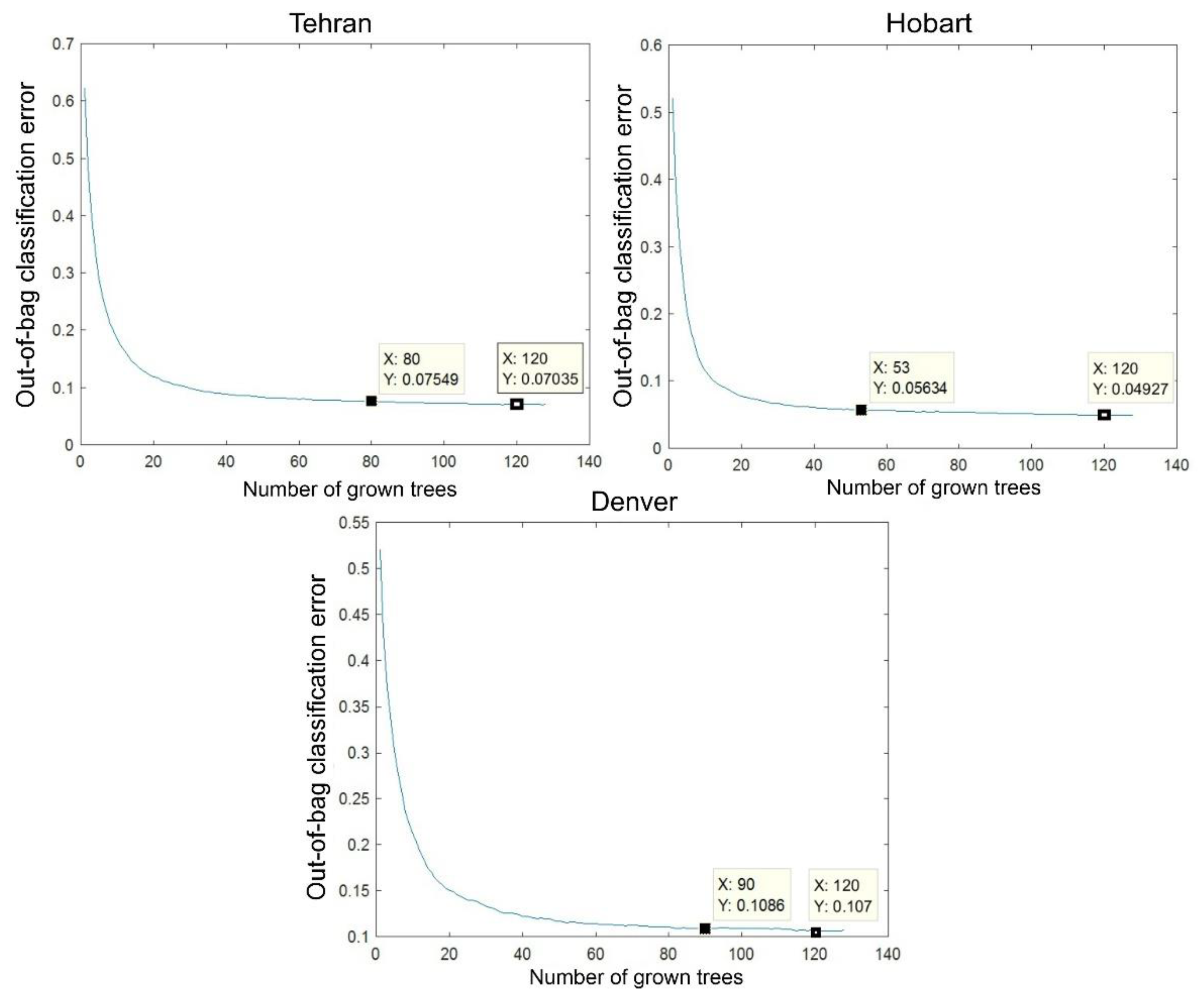
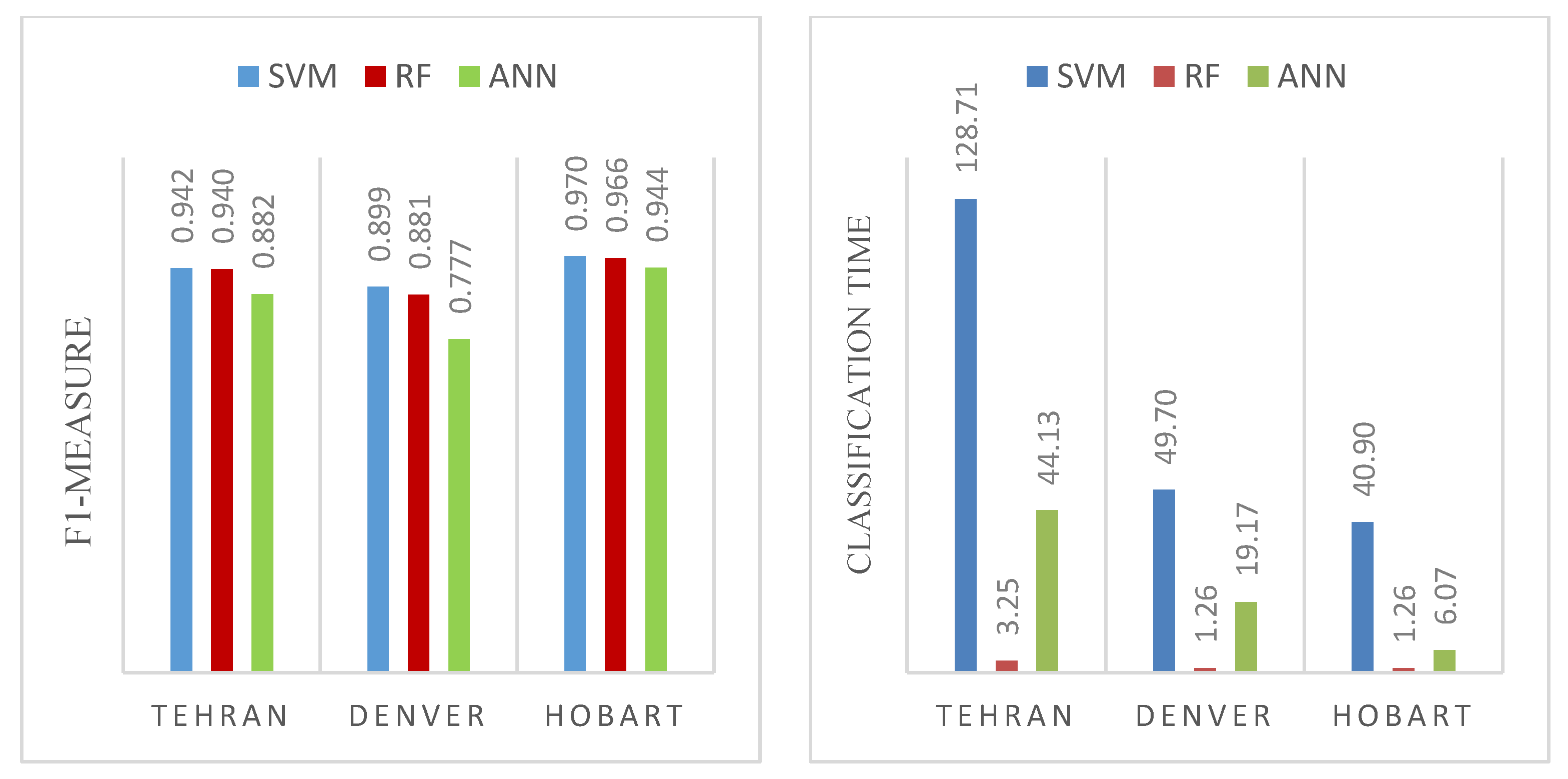
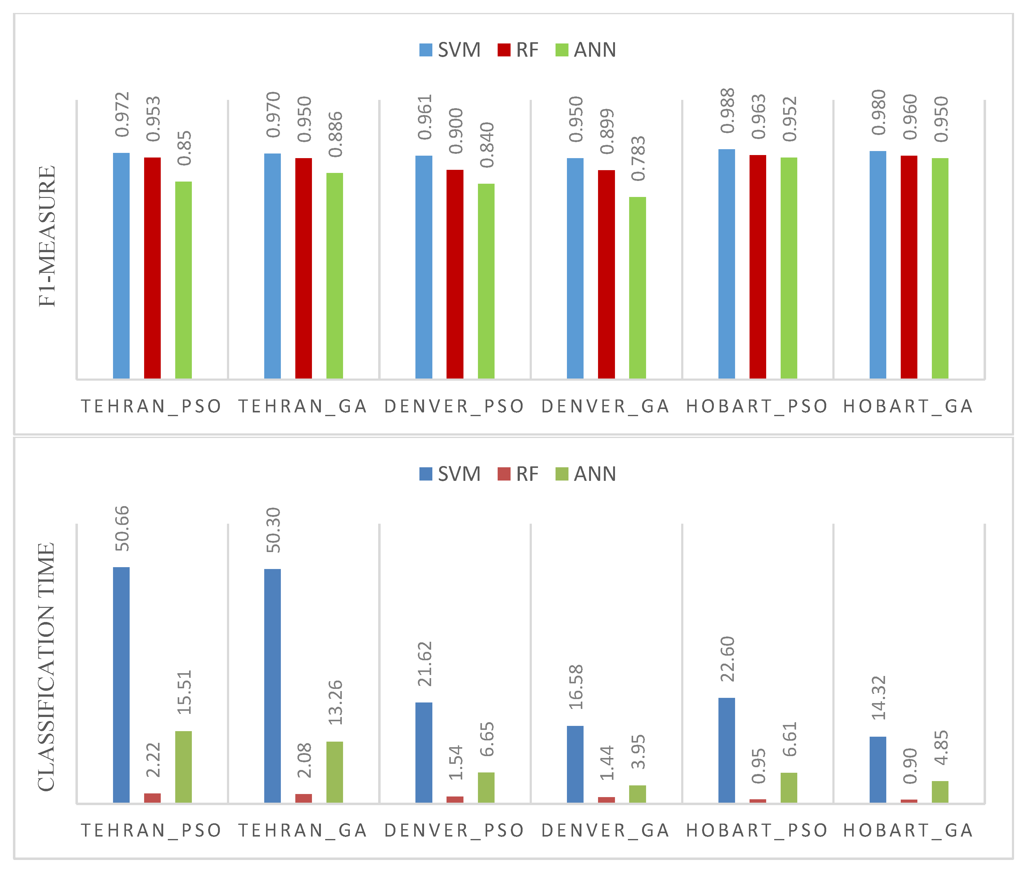
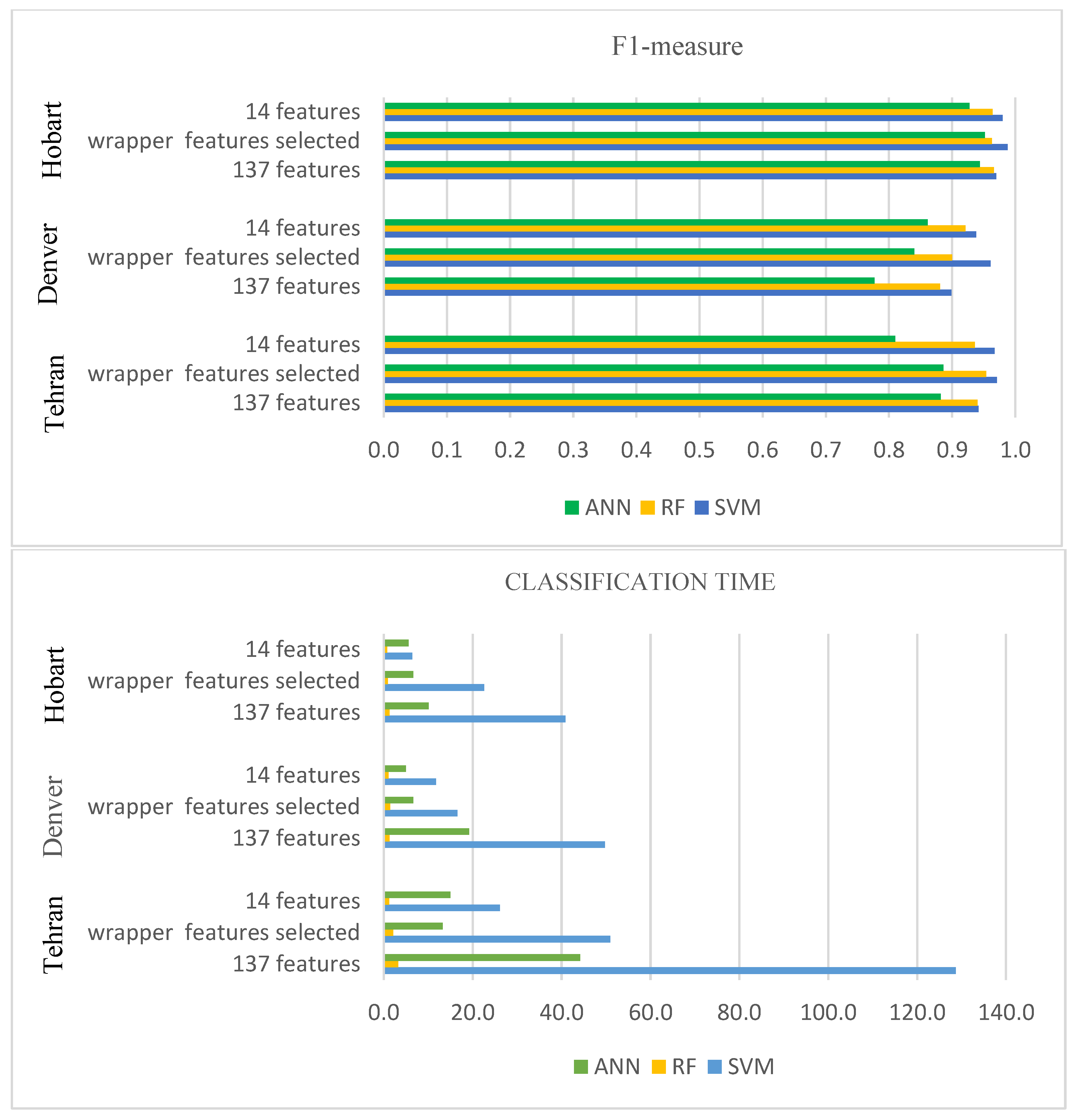
3. Results and Discussion

3.1. Multiscale Textural Feature Extraction

Identifying appropriate textural features is challenging since an efficient texture feature is a set of parameters such as texture measure, window size, spectral band, direction, and cell shift [12]. The influence of a textural feature in the classification increases with increasing spatial resolution or window size [76,77]. However, the solitary optimal window size for the exploitation of texture would not be adequate for images of urban scenes covering land use/cover classes with similar spectral behaviors. Therefore the multiscale texture analysis is appropriate for urban scenes [2,13]. In this study, five different window sizes (e.g., 5 × 5, 9 × 9, 17 × 17, 31 × 31, and 51 × 51); three directions of horizontal (0°), diagonal (45°), and vertical (90°); and four cell shifts of 3, 7, 15, and 30 pixels were tuned to implement the technique. All these configurations resulted in 136 features. It should be noted that the various directions and cell shifts are only restricted to the second-order textural parameters. For more information about how these cell shifts, directions, and window sizes were selected, see [13].
In order to adequately name each feature, the ‘ZX-A-B’ code was defined and used, where Z, X, A, and B are feature type, window size, cell shift, and direction or angle of the measuring filter, respectively. Table A7 presents all these 137 features used in this work, where the feature type ASM is for angular second moment, Cont is for contrast, Cor is for correlation, Dis is for dissimilarity, Ent is for entropy, Homo is for homogeneity, Var is for variance, Mean is for mean, and Pan is for panchromatic. For example, Cont9-7-45 represents a feature calculated using a contrast filter with a 9 × 9 window size and a 7-pixel cell shift in a diagonal direction.

3.2. Classification of Extracted Features

All the extracted features were input to the considered machine learning classifiers. Then the wrapper-based and filter-based optimization algorithms were applied to obtain the desired feature set. Scaled conjugate gradient (SCG) and the tangent sigmoid transfer, adaptable to GPU, were used as a network training method and transfer function. For the SVM classifier, we utilized radial basis function (RBF) kernel and grid search with 10-fold cross-validation to set the parameters of C and γ. Since RF is computationally productive and resistant to overfitting, n-tree can be chosen as large as possible [74,78]. In this study, the OOB error against the number of trees was used with 120 n-tree to reach the best approximation of n-tree for each image (Figure 3). This figure shows a slight difference between the out-of-bag classification error with 120 trees and the other cases with different tree numbers. Consequently, fewer trees were chosen for RF classification to decrease computational time and burden.
The 137 features were input to three classifiers, i.e., ANN, SVM, and RF, for three images (Tehran, Hobart, and Denver). The outputs were analyzed based on F1-measure [79,80,81,82,83,84,85] and processing time (Figure 4); the results indicated that SVM and ANN had the best and weakest F1-measure values. On the other hand, the slowest was SVM, while RF experienced the fastest performance. In addition, RF illustrated the most efficient consequences regarding classification accuracy and time since its F1-measure was approximately near that of SVM and it was also the most rapid one.
Though high-dimensional feature input may offer more information, the irrelevant, wasteful, and redundant ones decrease the processing speed and classification accuracy. Hence, the optimal feature dataset should be provided by eliminating the repetitious and irrational information to solve this problem. In the first step, GA and PSO were implemented as the wrapper-based feature selection methods to pursue the aim. Given that the wrapper-based process is highly time intensive, we employed parallel programming in the MATLAB environment to accelerate the performance. The GA and PSO parameter values shown in Table A8 and Table A9 were used in this study.
The number of features selected via the methods can be seen in Table 1. It should be noted that the time elapsed for the GA process in the three images, on average, was 4 h in comparison to 3 h for the PSO process.
Subsequently, these selected features were employed in the classifiers used in this study, and their results were investigated based on the classification time and accuracy (Figure 5). These results show that similar performance, in terms of accuracy and efficiency, can be achieved using only the optimally selected features. For all images, better classification F1-measure and faster processing time were achieved when using the input of selected features than using the original 137 input dataset. In addition, classification F1-measure values with PSO-selected features as inputs were higher than those with GA-selected features, but classifications with PSO-selected features required a longer processing time in all the trials.
In the second step, three filter-based feature selection approaches, namely NCA, relief-F, and MRMR, were conducted with wrapper-based selected features to select the best 10% (approximately 14 features) from the whole dataset (i.e., 137 features). The results are presented in Table A10. Then, the 14 optimally selected features were used to classify the three images. Table 2 presents the results from classification, including F1-measure values and overall processing time. It should be noted that the overall processing time was the summation of classification and filter-based processing time.
According to Table 2, the 14 optimal features provided by PSO_NCA and classified by SVM were the best combination for obtaining the highest classification accuracy in all intended images. While SVM was the most accurate classifier, RF was the most rapid. In addition, the combination PSO_NCA_RF (the qualified features produced by PSO and then minimized by NCA with classifying in RF) offered the most efficient overall time and F1-measure value in all three images. PSO, NCA, and SVM outperformed their counterparts for three images in terms of accuracy. Nonetheless, MRMR and RF indicated the best performance compared to their peer methods for these images in terms of processing speed. Meanwhile, as stated above, PSO was generally faster than GA.
In order to compare the classification accuracy and time per the input dataset, Figure 6 demonstrates the best output of each classifier and feature set for individual images. In all experiments, the F1-measure value increased with a decrease in input features from 137 to wrapper-based selected features. Moreover, this led to variations such as a slight decline or even a rise (in Denver for RF classifier) in wrapper-based results using the optimal feature datasets. The classification time, in all trials, was reduced with the optimum inputs. Although SVM and ANN’s process time depended on the input dataset, RF had a significantly minor sensitivity to the change in input. Overall, the most productive combination of dataset and classifier was the set of 14 optimal features and RF.

3.3. Analysis of Generalization

In order to investigate the generalization of the PSO_NCA feature set in other VHR satellite images classification, two images from Pléiades and WorldView-3 sensors over Melbourne and Rio de Janeiro were classified by the same classifiers (Table 3). Similar to the previous trials, while SVM provided the highest accuracy and process time, ANN led to the lowest F1-measure value and average processing time. On the other hand, RF, indicated as the fastest classifier with a satisfying F1-measure value of above 0.9, was regarded as the most productive method. The PSO_NCA feature set represented acceptable performance for the new images, the same as the former three data, indicating the high generalization capability.
While several studies [30,31,32] indicated that the wrapper-based methods outperformed filter-based algorithms, this study utilized both to achieve the dataset with proper size and good performance. Our results showed that the feature dataset selected by wrapper-based algorithms was still extensive and subsequently accompanied by high computational time. Therefore, the filter-based methods were employed to minimize the dataset achieved by wrapper-based algorithms by up to ten percent of the primary dataset. The results indicated that the wrapper features selected outperformed the original set (137 features) and the set of 14 features in classification accuracy. However, 14 features provided the fastest classification process and high classification accuracy in all experimented images.
On the other hand, while SVM and ANN experienced considerable fluctuations in performance with the change of feature input size, RF revealed slight declines in computational burden and classification performance. According to [2,13], the textural features utilized in this study can be effective in the shadowed area and for vertical objects’ (buildings and trees) extraction without the use of elevation features such as the digital elevation model (DEM) and the shadow effects. Therefore, the proposed methodologies can be used efficiently to extract buildings and trees with an average user accuracy of around 94% and 89% achieved with the PSO_NCA_RF dataset.

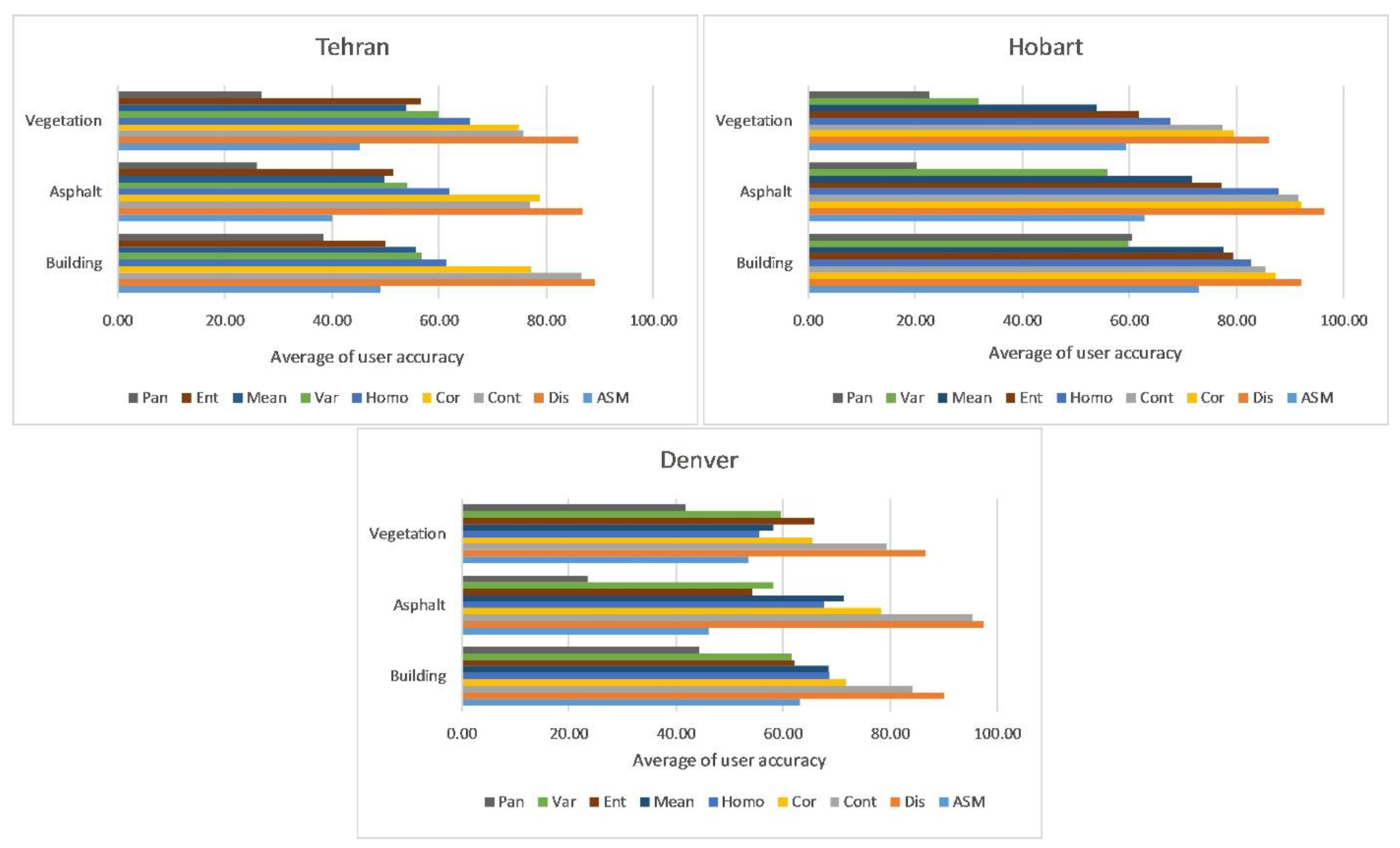
3.4. Feature Assessment

To investigate the role of the extracted features (Table A7) in the classification, five first-order feature datasets (the last column of Table A7) and 21 second-order feature datasets (columns 1–6 of Table A7), as well as the panchromatic band for Tehran, Hobart, and Denver’s images, were individually input to SVM. Then, the average user accuracies of three major classes, i.e., vegetation (tree, shrub, and lawn), asphalt (road, highway, and parking), and building (high-rise, low-rise, and commercial building), were calculated (Figure 7). The results presented that dissimilarity, contrast, and correlation played the most crucial role in the more-accurate extraction of the major classes in all experiments. The results were consistent with the final 14 optimal feature cases since these textural parameters constitute at least half of the selected features for GA_Relief-F, PSO_Relief-F, GA_NCA, and PSO_NCA datasets (Table A10). However, dissimilarity, contrast, and correlation had fewer shares in the cases of the feature sets selected by GA_MRMR and PSO_MRMR (Table A10), which induced weaker classification performance (Table 2). On the other hand, the feature sets of GA_Relief-F, PSO_Relief-F, and GA_NCA (Table A10) comprised features with small window sizes (5 × 5 and 9 × 9). As the bigger the window size of textural features is, the better the classification performance [2,13,76,77] is; the PSO_NCA dataset (Table A10) involving only the biggest window sizes (31 × 31 and 51 × 51) was accompanied by the most efficient classification performance (Table 2). Furthermore, the panchromatic band presented an acceptable performance as a single input compared to first- and second-order textural features in classification as a feature dataset (Figure 7). Accordingly, the panchromatic image had the potential to be involved in PSO_NCA as the most efficient feature dataset (Table A10).
The results showed that PSO outperformed GA in classification accuracy and computational time, similar to the case in previous works [33,86,87,88,89,90]. On the other hand, NCA was superior to its counterparts, the same as in [11,85], while MRMR provided the fastest process. Compared to a previous study [13] with identical study areas, input dataset (137 feature set), and classifier (ANN), the number of training samples was decreased by 41%, 43%, and 36% for Tehran, Hobart, and Denver images, respectively. This study dataset calculated the kappa value to compare the change extent, presenting a decrease in kappa by 0.07 for Tehran, 0.06 for Hobart, and 0.14 for Denver. This fact indicates the high sensitivity of ANN to training samples compared to SVM and RF, which is consistent with the results of previous works by [44,49,91,92].
Moreover, RF and ANN were the most and the least efficient methods among AI-based classifiers, as reported in the literature [39,43,72,93,94,95]. RF had the most rapid classification process. Additionally, although SVM and ANN’s process time depended on the number of input features, RF had a significantly minor sensitivity to the number of input features. Accordingly, RF was the most robust classifier, consistent with [95]. Several studies based on GLCM textural features reported entropy, angular second moment, and contrast as the most valuable features in classification [2,13,96,97,98,99,100]. However, in this study, dissimilarity, contrast, and correlation showed the most contributing role in the classification performance based on feature evaluation in the classification and comparing its results with the optimal features selected by optimization approaches.
The results indicated the validity of the optimum feature input by presenting the F1-measure value of larger than 0.9 for the classification process. Furthermore, data processing time and burden were considerably reduced in the classification process, which is one of the merits of the proposed method compared to the previous works [2,13,72,101]. On the other hand, providing a generalizable dataset for classification can be considered the most significant achievement of this research, which has not been applied in previous studies.
While the approach in this study has significantly decreased the computational time and burden and represented a robust and fast method to classify different landscapes in VHR imagery for urban areas, the extraction of training samples has remained challenging and time consuming. The sampling issue can be regarded as the drawback of this study, which is necessary for machine learning supervised classification algorithms. Nevertheless, the downside can be addressed by convolutional neural networks (CNNs) independent of training samples’ exploitation.

4. Conclusions

Feature selection to reduce redundancies for efficient classification is necessary but usually time consuming and challenging. This study offered proper guidelines for selecting textual features for more accurate land use/cover classification. Accordingly, 136 multiscale textural features were generated from each test image. These features, plus the panchromatic band, were used in an AI-based selection process. Firstly, the feature set was optimized by PSO and GA as per the wrapper-based feature selection algorithms. The selected features were then optimally reduced by ten percent of the initial features extracted by filter-based FS methods, including NCA, relief-F, and MRMR.
Moreover, the performance of each feature set was investigated with results using SVM, RF, and ANN classifiers. Finally, the efficiency of the optimum feature set was analyzed by using new images and compared to those in the preliminary trials. The experiments showed that RF, PSO, and NCA were superior to their counterparts in terms of productivity. In the classification performance, dissimilarity, contrast, and correlation features outperformed other GLCM textural features and panchromatic bands. Contrary to SVM and ANN, RF indicated a minor sensitivity to the number of input features in term of implementation time. To conclude, the set of 14 optimal features (including 13 textural features and the panchromatic band) and RF classifier performed as the most optimum combination for classifying VHR images of urban areas. In the future, the role of this feature dataset in the performance of deep learning approaches can be further investigated.

Author Contributions

Conceptualization, M.S.; methodology, M.S., S.H. and R.S.-H.; programming, M.S.; validation, all authors; format analysis, all; writing, all authors; supervision, all authors. All authors have read and agreed to the published version of the manuscript.

Funding

This research received no external funding.

Data Availability Statement

The data, except for Tehran image, used in this paper were provided from MAXAR (formerly Digital Globe) (www.maxar.com) few years ago. Basir Remote Sensing Institute (www.basir-rsi.ir) also supplied the Tehran data.

Acknowledgments

The authors would like to thank MAXAR (formerly Digital Globe) Company and Basir Remote Sensing Institute for providing the VHR satellite images.

Conflicts of Interest

The authors declare no conflict of interest.

Appendix A

Table A1. Characteristics of satellite images utilized in this study.
Image Information
SatelliteDimension
(Pixels)
Location
(Based on Figure 2)
Spatial res. for PanchromaticSpatial res. for MultispectralAcquisition Date and TimeCenter Point Coordinates
Worldview-21040 × 695Tehran (Iran) (A)0.5 m2 m4 December 2010
7:15
35°44′46.85″N 51°15′38.92″E
GeoEye-1901 × 588Hobart (Australia) (E)0.5 m2 m5 March 2013
13:25
42°47′79″S 147°14′53.7″E
QuickBird679 × 646Denver (USA) (C)0.6 m2.4 m4 July 2005
18:01
40°01′20.04″N
105°17′29.5″W
Pléiades1119 × 634Melbourne (Australia) (D)0.5 m2 m25 February 2012
14:52
37°49′50.33″S 144°57′50.94″E
WorldView-31290 × 664Rio de Janeiro (Brazil) (B)0.31 m1.24 m2 May 2016
13:12
22°57′22.89″S
43°10′42.20″W

Appendix B

Table A2. Training and test samples for each class in the Tehran image.
Worldview-2 ClassesTraining Samples (Pixel)Test Samples (Pixel)
Bare soil112812,974
Lawn343139,459
Highway590067,851
Parking324637,539
Low-rise building324137,271
Road596668,604
Sports facility164818,949
High-rise building267330,737
Tree375943,225
Sidewalk136115,648
Shrub491056,471
Total ROIs37,263428,728
Table A3. Training and test samples for each class in the Denver image.
QuickBird ClassesTraining Samples (Pixel)Test Samples (Pixel)
Lawn369742,515
Highway122414,078
Parking320834,826
Low-rise building190722,661
Road247728,489
Commercial building264930,467
Tree768088,323
Total ROIs22,752261,359
Table A4. Training and test samples for each class in the Hobart image.
GeoEye-1 ClassesTraining Samples (Pixel)Test Samples (Pixel)
Bare soil616670,912
Lawn155317,863
Highway167119,219
Parking101611,681
Low-rise building250928,856
Road311535,820
Sports facility6117023
Commercial building259029,788
Tree311735,846
Total ROIs22,348257,008
Table A5. Training and test samples for each class in the Melbourne image.
Pléiades ClassesTraining Samples (Pixel)Test Samples (Pixel)
Lawn194922,409
Highway317636,527
Parking162318,670
Low-rise building11,319130,164
Road850597,808
Sports facility3033480
High-rise building510830,737
Tree353340,626
Railway194922,418
Total ROIs37,465402,839
Table A6. Training and test samples for each class in the Rio image.
WorldView-3 ClassesTrain Samples (Pixel)Test Samples (Pixel)
Bare soil141816,306
Lawn5115876
Highway186021,390
Parking162518,691
Low-rise building768088,321
Road377443,398
High-rise building427349,136
Tree466053,585
Shrub871000
Total ROIs25,888297,703

Appendix C

Table A7. All the textural features, as well as the panchromatic band, were coded based on the proposed protocol used in the classification (137 features).
Input Features
ASM5_3_0Cont5_3_0Cor5_3_0Dis5_3_0Ent5_3_0Homo5_3_0Mean5
ASM5_3_45Cont5_3_45Cor5_3_45Dis5_3_45Ent5_3_45Homo5_3_45Mean9
ASM5_3_90Cont5_3_90Cor5_3_90Dis5_3_90Ent5_3_90Homo5_3_90Mean17
ASM9_7_0Cont9_7_0Cor9_7_0Dis9_7_0Ent9_7_0Homo9_7_0Mean31
ASM9_7_45Cont9_7_45Cor9_7_45Dis9_7_45Ent9_7_45Homo9_7_45Mean51
ASM9_7_90Cont9_7_90Cor9_7_90Dis9_7_90Ent9_7_90Homo9_7_90Var5
ASM17_15_0Cont17_15_0Cor17_15_0Dis17_15_0Ent17_15_0Homo17_15_0Var9
ASM17_15_45Cont17_15_45Cor17_15_45Dis17_15_45Ent17_15_45Homo17_15_45Var17
ASM17_15_90Cont17_15_90Cor17_15_90Dis17_15_90Ent17_15_90Homo17_15_90Var31
ASM31_15_0Cont31_15_0Cor31_15_0Dis31_15_0Ent31_15_0Homo31_15_0Var51
ASM31_15_45Cont31_15_45Cor31_15_45Dis31_15_45Ent31_15_45Homo31_15_45Pan
ASM31_15_90Cont31_15_90Cor31_15_90Dis31_15_90Ent31_15_90Homo31_15_90
ASM31_30_0Cont31_30_0Cor31_30_0Dis31_30_0Ent31_30_0Homo31_30_0
ASM31_30_45Cont31_30_45Cor31_30_45Dis31_30_45Ent31_30_45Homo31_30_45
ASM31_30_90Cont31_30_90Cor31_30_90Dis31_30_90Ent31_30_90Homo31_30_90
ASM51_15_0Cont51_15_0Cor51_15_0Dis51_15_0Ent51_15_0Homo51_15_0
ASM51_15_45Cont51_15_45Cor51_15_45Dis51_15_45Ent51_15_45Homo51_15_45
ASM51_15_90Cont51_15_90Cor51_15_90Dis51_15_90Ent51_15_90Homo51_15_90
ASM51_30_0Cont51_30_0Cor51_30_0Dis51_30_0Ent51_30_0Homo51_30_0
ASM51_30_45Cont51_30_45Cor51_30_45Dis51_30_45Ent51_30_45Homo51_30_45
ASM51_30_90Cont51_30_90Cor51_30_90Dis51_30_90Ent51_30_90Homo51_30_90

Appendix D

Table A8. Parameters used in GA for selecting optimum features.
GA ParameterValue
Population size60
Elite count2
Fitness functionKNN-based classification accuracy
Number of generations30
Mutation probability0.1
Crossover probability0.8
Crossover typeUnique
Table A9. Parameters used in PSO for selecting optimum features.
PSO ParameterValue
Population size60
Fitness functionKNN-based classification accuracy
Maximum iteration30
C12
C22

Appendix E

Table A10. Filter-based methods from wrapper-based results identified the last 14 optimal features.
Name of Selection MethodsContent of Optimal Features
GA_Relief-FMean31, Mean51, Mean9, Cor51_30_0, Cor51_15_90, Cor51_30_90, Cor31_15_45, Cor31_30_90, Dis51_30_45, Dis51_15_90, Cont51_15_90, Ent51_15_0, Ent31_15_45, Homo51_15_90,
PSO_Relief-FMean51, Mean31, Mean5, Mean9, Cor51_15_90, Cor51_30_0, Cor51_15_0, Cor31_15_45, Cor51_30_90, Cor31_15_0, Cont51_15_90, Cont51_15_0, Dis51_15_90, Dis51_30_45
GA_NCAMean51, Mean31, Mean5, Cor51_30_0, Cor51_15_90, Cor51_15_0, Cor31_15_45, Homo51_15_45, Homo31_15_90, Dis51_30_45, Dis31_15_45, Dis51_15_45, Var31, Ent31_15_45
PSO_NCAMean51, Mean31, Cor51_15_90, Cor51_15_0, Cor51_30_0, Cor51_30_90, Cor31_15_0, Cor31_15_45, Var31, Dis51_30_45, Cont51_15_0, Cont51_15_45, Homo51_15_90, Pan
GA_MRMRMean9, Mean31, Mean5, Cor51_30_0, Cor51_15_45, Asm9_7_0, Asm51_15_45, Asm17_15_90, Cont31_30_0, Cont9_7_90, Dis51_15_90, Dis51_30_90, Var31, Var9
PSO_MRMRMean9, Mean5, Mean31, Mean17, Cor31_15_0, Cor51_15_90, Cor5_3_0, Cor31_15_45, Asm9_7_0, Cont51_15_90, Var31, Ent51_30_45, Var31, Pan

Appendix F

Figure A1. The images and their classification maps of (A) (Tehran/WorldView-2), (B) (Hobart/GeoEye-1), (C) (Melbourne/Pléiades), (D) (Rio/WorldView-3), and (E) (Denver/QuickBird), by SVM with PSO_NCA input dataset.
Remotesensing 14 02097 g0a1aRemotesensing 14 02097 g0a1b

References

  1. Gong, P.; Marceau, D.J.; Howarth, P.J. A comparison of spatial feature extraction algorithms for land-use classification with SPOT HRV data. Remote Sens. Environ. 1992, 40, 137–151. [Google Scholar] [CrossRef]
  2. Pacifici, F.; Chini, M.; Emery, W. A neural network approach using multi-scale textural metrics from very high-resolution panchromatic imagery for urban land-use classification. Remote Sens. Environ. 2009, 113, 1276–1292. [Google Scholar] [CrossRef]
  3. Clausi, D.; Yue, B. Comparing Cooccurrence Probabilities and Markov Random Fields for Texture Analysis of SAR Sea Ice Imagery. IEEE Trans. Geosci. Remote Sens. 2004, 42, 215–228. [Google Scholar] [CrossRef]
  4. Kupidura, P. The Comparison of Different Methods of Texture Analysis for Their Efficacy for Land Use Classification in Satellite Imagery. Remote Sens. 2019, 11, 1233. [Google Scholar] [CrossRef] [Green Version]
  5. Tuceryan, M.; Jain, A.K. Texture analysis. In Handbook of Pattern Recognition and Computer Vision; World Scientific: Singapore, 1993; pp. 235–276. [Google Scholar]
  6. Anys, H.; He, D.-C. Evaluation of textural and multipolarization radar features for crop classification. IEEE Trans. Geosci. Remote Sens. 1995, 33, 1170–1181. [Google Scholar] [CrossRef]
  7. Soares, J.V.; Rennó, C.D.; Formaggio, A.R.; Yanasse, C.D.C.F.; Frery, A.C. An investigation of the selection of texture features for crop discrimination using SAR imagery. Remote Sens. Environ. 1997, 59, 234–247. [Google Scholar] [CrossRef]
  8. Kim, M.; Madden, M.; Warner, T.A. Forest Type Mapping using Object-specific Texture Measures from Multispectral Ikonos Imagery. Photogramm. Eng. Remote Sens. 2009, 75, 819–829. [Google Scholar] [CrossRef] [Green Version]
  9. Jin, Y.; Liu, X.; Chen, Y.; Liang, X. Land-cover mapping using Random Forest classification and incorporating NDVI time-series and texture: A case study of central Shandong. Int. J. Remote Sens. 2018, 39, 8703–8723. [Google Scholar] [CrossRef]
  10. Ferreira, M.P.; Wagner, F.H.; Aragão, L.E.O.C.; Shimabukuro, Y.E.; de Souza Filho, C.R. Tree species classification in tropical forests using visible to shortwave infrared WorldView-3 images and texture analysis. ISPRS J. Photogramm. Remote Sens. 2019, 149, 119–131. [Google Scholar] [CrossRef]
  11. Ruiz Hernandez, I.E.; Shi, W. A Random Forests classification method for urban land-use mapping integrating spatial metrics and texture analysis. Int. J. Remote Sens. 2018, 39, 1175–1198. [Google Scholar] [CrossRef]
  12. Mishra, V.N.; Prasad, R.; Rai, P.K.; Vishwakarma, A.K.; Arora, A. Performance evaluation of textural features in improving land use/land cover classification accuracy of heterogeneous landscape using multi-sensor remote sensing data. Earth Sci. Inform. 2018, 12, 71–86. [Google Scholar] [CrossRef]
  13. Saboori, M.; Torahi, A.A.; Bakhtyari, H.R.R. Combining multi-scale textural features from the panchromatic bands of high spatial resolution images with ANN and MLC classification algorithms to extract urban land uses. Int. J. Remote Sens. 2019, 40, 8608–8634. [Google Scholar] [CrossRef]
  14. Bramhe, V.S.; Ghosh, S.K.; Garg, P.K. Extraction of built-up areas from Landsat-8 OLI data based on spectral-textural information and feature selection using support vector machine method. Geocarto Int. 2019, 35, 1067–1087. [Google Scholar] [CrossRef]
  15. Guyon, I.; Weston, J.; Barnhill, S.; Vapnik, V. Gene Selection for Cancer Classification using Support Vector Machines. Mach. Learn. 2002, 46, 389–422. [Google Scholar] [CrossRef]
  16. Mundra, P.A.; Rajapakse, J.C. SVM-RFE with relevancy and redundancy criteria for gene selection. In Proceedings of the IAPR International Workshop on Pattern Recognition in Bioinformatics, Singapore, 1–2 October 2007; pp. 242–252. [Google Scholar]
  17. Jaffel, Z.; Farah, M. A symbiotic organisms search algorithm for feature selection in satellite image classification. In Proceedings of the 2018 4th International Conference on Advanced Technologies for Signal and Image Processing (ATSIP), Sousse, Tunisia, 21–24 March 2018; pp. 1–5. [Google Scholar]
  18. Ranjbar, H.R.; Ardalan, A.A.; Dehghani, H.; Saradjian, M.R. Using high-resolution satellite imagery to provide a relief priority map after earthquake. Nat. Hazards 2017, 90, 1087–1113. [Google Scholar] [CrossRef]
  19. Genuer, R.; Poggi, J.-M.; Tuleau-Malot, C. VSURF: An R Package for Variable Selection Using Random Forests. R J. 2015, 7, 19–33. [Google Scholar] [CrossRef] [Green Version]
  20. Georganos, S.; Grippa, T.; VanHuysse, S.; Lennert, M.; Shimoni, M.; Kalogirou, S.; Wolff, E. Less is more: Optimizing classification performance through feature selection in a very-high-resolution remote sensing object-based urban application. GISci. Remote Sens. 2017, 55, 221–242. [Google Scholar] [CrossRef]
  21. Saeys, Y.; Inza, I.; Larrañaga, P. A review of feature selection techniques in bioinformatics. Bioinformatics 2007, 23, 2507–2517. [Google Scholar] [CrossRef] [Green Version]
  22. Scott, D.W. Multivariate Density Estimation: Theory, Practice, and Visualization; John Wiley & Sons: Hoboken, NJ, USA, 2015. [Google Scholar]
  23. Jindal, P.; Kumar, D. A review on dimensionality reduction techniques. Comput. Sci. Int. J. Comput. Appl. 2017, 173, 42–46. [Google Scholar] [CrossRef]
  24. Abd-Alsabour, N.J.J.C. On the Role of Dimensionality Reduction. J. Comput. 2018, 13, 571–579. [Google Scholar] [CrossRef]
  25. Zebari, R.; AbdulAzeez, A.; Zeebaree, D.; Zebari, D.; Saeed, J. A Comprehensive Review of Dimensionality Reduction Techniques for Feature Selection and Feature Extraction. J. Appl. Sci. Technol. Trends 2020, 1, 56–70. [Google Scholar] [CrossRef]
  26. Liu, H.; Yu, L. Toward integrating feature selection algorithms for classification and clustering. IEEE Trans. Knowl. Data Eng. 2005, 17, 491–502. [Google Scholar]
  27. Zhu, Z.; Ong, Y.-S.; Dash, M. Wrapper–filter feature selection algorithm using a memetic framework. IEEE Trans. Syst. ManCybern. Part B (Cybern.) 2007, 37, 70–76. [Google Scholar] [CrossRef]
  28. Mahrooghy, M.; Younan, N.H.; Anantharaj, V.G.; Aanstoos, J.; Yarahmadian, S. On the Use of the Genetic Algorithm Filter-Based Feature Selection Technique for Satellite Precipitation Estimation. IEEE Geosci. Remote Sens. Lett. 2012, 9, 963–967. [Google Scholar] [CrossRef]
  29. Tamimi, E.; Ebadi, H.; Kiani, A. Evaluation of different metaheuristic optimization algorithms in feature selection and parameter determination in SVM classification. Arab. J. Geosci. 2017, 10, 478. [Google Scholar] [CrossRef]
  30. Zhao, H.; Min, F.; Zhu, W. Cost-Sensitive Feature Selection of Numeric Data with Measurement Errors. J. Appl. Math. 2013, 2013, 1–13. [Google Scholar] [CrossRef]
  31. Jain, D.; Singh, V. Feature selection and classification systems for chronic disease prediction: A review. Egypt. Inform. J. 2018, 19, 179–189. [Google Scholar] [CrossRef]
  32. Jamali, A. Evaluation and comparison of eight machine learning models in land use/land cover mapping using Landsat 8 OLI: A case study of the northern region of Iran. SN Appl. Sci. 2019, 1, 1448. [Google Scholar] [CrossRef] [Green Version]
  33. Naeini, A.A.; Babadi, M.; Mirzadeh, S.M.J.; Amini, S. Particle Swarm Optimization for Object-Based Feature Selection of VHSR Satellite Images. IEEE Geosci. Remote Sens. Lett. 2018, 15, 379–383. [Google Scholar] [CrossRef]
  34. Hamedianfar, A.; Shafri, H.Z.M. Integrated approach using data mining-based decision tree and object-based image analysis for high-resolution urban mapping of WorldView-2 satellite sensor data. J. Appl. Remote Sens. 2016, 10, 025001. [Google Scholar] [CrossRef]
  35. Wu, B.; Chen, C.; Kechadi, T.M.; Sun, L. A comparative evaluation of filter-based feature selection methods for hyper-spectral band selection. Int. J. Remote Sens. 2013, 34, 7974–7990. [Google Scholar] [CrossRef]
  36. Malan, N.S.; Sharma, S.J. Feature selection using regularized neighbourhood component analysis to enhance the classification performance of motor imagery signals. Comput. Biol. Med. 2019, 107, 118–126. [Google Scholar] [CrossRef] [PubMed]
  37. Ren, J.; Wang, R.; Liu, G.; Feng, R.; Wang, Y.; Wu, W. Partitioned Relief-F Method for Dimensionality Reduction of Hyperspectral Images. Remote Sens. 2020, 12, 1104. [Google Scholar] [CrossRef] [Green Version]
  38. Atkinson, P.M.; Tatnall, A.R.L. Introduction Neural networks in remote sensing. Int. J. Remote Sens. 1997, 18, 699–709. [Google Scholar] [CrossRef]
  39. Xie, Z.; Chen, Y.; Lu, D.; Li, G.; Chen, E. Classification of Land Cover, Forest, and Tree Species Classes with ZiYuan-3 Multispectral and Stereo Data. Remote Sens. 2019, 11, 164. [Google Scholar] [CrossRef] [Green Version]
  40. Mukherjee, A.; Kumar, A.A.; Ramachandran, P.; Sensing, R. Development of new index-based methodology for extraction of built-up area from landsat7 imagery: Comparison of performance with svm, ann, and existing indices. IEEE Trans. Geosci. Remote Sens. 2020, 59, 1592–1603. [Google Scholar] [CrossRef]
  41. Civco, D.L. Artificial neural networks for land-cover classification and mapping. Geogr. Inf. Syst. 1993, 7, 173–186. [Google Scholar] [CrossRef]
  42. Zhang, C.; Sargent, I.M.J.; Pan, X.; Li, H.; Gardiner, A.; Hare, J.; Atkinson, P.M. Joint Deep Learning for land cover and land use classification. Remote Sens. Environ. 2018, 221, 173–187. [Google Scholar] [CrossRef] [Green Version]
  43. Talukdar, S.; Singha, P.; Mahato, S.; Praveen, B.; Rahman, A. Dynamics of ecosystem services (ESs) in response to land use land cover (LU/LC) changes in the lower Gangetic plain of India. Ecol. Indic. 2020, 112, 106121. [Google Scholar] [CrossRef]
  44. Rogan, J.; Franklin, J.; Stow, D.; Miller, J.; Woodcock, C.; Roberts, D. Mapping land-cover modifications over large areas: A comparison of machine learning algorithms. Remote Sens. Environ. 2008, 112, 2272–2283. [Google Scholar] [CrossRef]
  45. Camargo, F.F.; Sano, E.E.; Almeida, C.M.; Mura, J.C.; Almeida, T.J.R.S. A comparative assessment of machine-learning techniques for land use and land cover classification of the Brazilian tropical savanna using ALOS-2/PALSAR-2 polarimetric images. Remote Sens. 2019, 11, 1600. [Google Scholar] [CrossRef] [Green Version]
  46. Vohra, R.; Tiwari, K.C. Comparative Analysis of SVM and ANN Classifiers using Multilevel Fusion of Multi-Sensor Data in Urban Land Classification. Sens. Imaging 2020, 21, 1–21. [Google Scholar] [CrossRef]
  47. Ghasemi, M.; Karimzadeh, S.; Feizizadeh, B. Urban classification using preserved information of high dimensional textural features of Sentinel-1 images in Tabriz, Iran. Earth Sci. Inform. 2021, 14, 1745–1762. [Google Scholar] [CrossRef]
  48. Rodriguez-Galiano, V.F.; Ghimire, B.; Rogan, J.; Chica-Olmo, M.; Rigol-Sanchez, J.P. An assessment of the effectiveness of a random forest classifier for land-cover classification. ISPRS J. Photogramm. Remote Sens. 2012, 67, 93–104. [Google Scholar] [CrossRef]
  49. Ghosh, A.; Joshi, P. A comparison of selected classification algorithms for mapping bamboo patches in lower Gangetic plains using very high resolution WorldView 2 imagery. Int. J. Appl. Earth Obs. Geoinformation 2014, 26, 298–311. [Google Scholar] [CrossRef]
  50. Mountrakis, G.; Im, J.; Ogole, C.; Sensing, R. Support vector machines in remote sensing: A review. ISPRS J. Photogramm. Remote Sens. 2011, 66, 247–259. [Google Scholar] [CrossRef]
  51. Ma, L.; Li, M.; Ma, X.; Cheng, L.; Du, P.; Liu, Y. A review of supervised object-based land-cover image classification. ISPRS J. Photogramm. Remote Sens. 2017, 130, 277–293. [Google Scholar] [CrossRef]
  52. Sheykhmousa, M.; Mahdianpari, M.; Ghanbari, H.; Mohammadimanesh, F.; Ghamisi, P.; Homayouni, S. Support Vector Machine Versus Random Forest for Remote Sensing Image Classification: A Meta-Analysis and Systematic Review. IEEE J. Sel. Top. Appl. Earth Obs. Remote Sens. 2020, 13, 6308–6325. [Google Scholar] [CrossRef]
  53. Deng, J.S.; Wang, K.; Deng, Y.H.; Qi, G.J. PCA-based land-use change detection and analysis using multitemporal and multisensor satellite data. Int. J. Remote Sens. 2008, 29, 4823–4838. [Google Scholar] [CrossRef]
  54. Foody, G.M. Status of land cover classification accuracy assessment. Remote Sens. Environ. 2002, 80, 185–201. [Google Scholar] [CrossRef]
  55. Jensen, J.R. Introductory Digital Image Processing, 3rd ed.; Prentice Hall: Upper Saddle River, NJ, USA, 2005. [Google Scholar]
  56. Haralick, R.M.; Shanmugam, K.; Dinstein, I.H. Textural Features for Image Classification. IEEE Trans. Syst. Man Cybern. 1973, SMC-3, 610–621. [Google Scholar] [CrossRef] [Green Version]
  57. Grizonnet, M.; Michel, J.; Poughon, V.; Inglada, J.; Savinaud, M.; Cresson, R. Orfeo ToolBox: Open source processing of remote sensing images. Open Geospatial Data Softw. Stand. 2017, 2, 15. [Google Scholar] [CrossRef] [Green Version]
  58. Dash, M.; Liu, H. Feature selection for classification. Intell. Data Anal. 1997, 1, 131–156. [Google Scholar] [CrossRef]
  59. Huang, X.; Wu, L.; Ye, Y.; Intelligence, A. A review on dimensionality reduction techniques. Int. J. Pattern Recognit. Artif. Intell. 2019, 33, 1950017. [Google Scholar] [CrossRef]
  60. Khaire, U.M.; Dhanalakshmi, R. Stability of feature selection algorithm: A review. J. King Saud Univ.-Comput. Inf. Sci. 2019, 34, 1060–1073. [Google Scholar] [CrossRef]
  61. Kira, K.; Rendell, L.A. A practical approach to feature selection. In Machine Learning Proceedings; Elsevier: Amsterdam, The Netherlands, 1992; pp. 249–256. [Google Scholar]
  62. Yang, W.; Wang, K.; Zuo, W. Neighborhood Component Feature Selection for High-Dimensional Data. J. Comput. 2012, 7, 161–168. [Google Scholar] [CrossRef]
  63. Li, P.; Hong, Z.; Zuxun, Z.; Jianqing, Z. Genetic feature selection for texture classification. Geo-Spat. Inf. Sci. 2004, 7, 162–166. [Google Scholar] [CrossRef]
  64. Mather, P.; Tso, B. Classification Methods for Remotely Sensed Data; CRC Press: Boca Raton, FL, USA, 2016. [Google Scholar]
  65. Khodaverdizahraee, N.; Rastiveis, H.; Jouybari, A. Segment-by-segment comparison technique for earthquake-induced building damage map generation using satellite imagery. Int. J. Disaster Risk Reduct. 2020, 46, 101505. [Google Scholar] [CrossRef]
  66. Kennedy, J.; Eberhart, R. Particle swarm optimization. In Proceedings of the ICNN’95-International Conference on Neural Networks, Perth, WA, Australia, 27 November–1 December 1995; pp. 1942–1948. [Google Scholar]
  67. Sammut, C.; Webb, G.I. Encyclopedia of Machine Learning; Springer Science & Business Media: Berlin/Heidelberg, Germany, 2011. [Google Scholar]
  68. Doma, M.I.; Sedeek, A.A. Comparison of PSO, GAs and analytical techniques in second-order design of deformation monitoring networks. J. Appl. Geod. 2014, 8, 21–30. [Google Scholar] [CrossRef]
  69. Jia, F.; Lichti, D. A comparison of simulated annealing, genetic algorithm and particle swarm optimization in optimal first-order design of indoor tls networks. ISPRS Ann. Photogramm. Remote Sens. Spat. Inf. Sci. 2017, IV-2/W4, 75–82. [Google Scholar] [CrossRef] [Green Version]
  70. Liou, Y.-A.; Tzeng, Y.; Chen, K. A neural-network approach to radiometric sensing of land-surface parameters. IEEE Trans. Geosci. Remote Sens. 1999, 37, 2718–2724. [Google Scholar] [CrossRef]
  71. Liu, X.; He, J.; Yao, Y.; Zhang, J.; Liang, H.; Wang, H.; Hong, Y. Classifying urban land use by integrating remote sensing and social media data. Int. J. Geogr. Inf. Sci. 2017, 31, 1675–1696. [Google Scholar] [CrossRef]
  72. Mao, W.; Lu, D.; Hou, L.; Liu, X.; Yue, W. Comparison of Machine-Learning Methods for Urban Land-Use Mapping in Hangzhou City, China. Remote Sens. 2020, 12, 2817. [Google Scholar] [CrossRef]
  73. Du, S.; Zhang, F.; Zhang, X. Semantic classification of urban buildings combining VHR image and GIS data: An improved random forest approach. ISPRS J. Photogramm. Remote Sens. 2015, 105, 107–119. [Google Scholar] [CrossRef]
  74. Belgiu, M.; Drăguţ, L. Random forest in remote sensing: A review of applications and future directions. ISPRS J. Photogramm. Remote Sens. 2016, 114, 24–31. [Google Scholar] [CrossRef]
  75. Feng, Q.; Liu, J.; Gong, J. UAV Remote Sensing for Urban Vegetation Mapping Using Random Forest and Texture Analysis. Remote Sens. 2015, 7, 1074–1094. [Google Scholar] [CrossRef] [Green Version]
  76. Shaban, M.A.; Dikshit, O. Improvement of classification in urban areas by the use of textural features: The case study of Lucknow city, Uttar Pradesh. Int. J. Remote Sens. 2001, 22, 565–593. [Google Scholar] [CrossRef]
  77. Lu, D.; Hetrick, S.; Moran, E. Land Cover Classification in a Complex Urban-Rural Landscape with QuickBird Imagery. Photogramm. Eng. Remote Sens. 2010, 76, 1159–1168. [Google Scholar] [CrossRef] [Green Version]
  78. Lawrence, R.L.; Wood, S.D.; Sheley, R.L. Mapping invasive plants using hyperspectral imagery and Breiman Cutler classifications (randomForest). Remote Sens. Environ. 2006, 100, 356–362. [Google Scholar] [CrossRef]
  79. Li, X.; Chen, W.; Cheng, X.; Wang, L. A Comparison of Machine Learning Algorithms for Mapping of Complex Surface-Mined and Agricultural Landscapes Using ZiYuan-3 Stereo Satellite Imagery. Remote Sens. 2016, 8, 514. [Google Scholar] [CrossRef] [Green Version]
  80. Zhou, T.; Pan, J.; Zhang, P.; Wei, S.; Han, T. Mapping Winter Wheat with Multi-Temporal SAR and Optical Images in an Urban Agricultural Region. Sensors 2017, 17, 1210. [Google Scholar] [CrossRef] [PubMed]
  81. Guirado, E.; Tabik, S.; Rivas, M.L.; Alcaraz-Segura, D.; Herrera, F.J.B. Automatic whale counting in satellite images with deep learning. Sci. Rep. 2018, 44367. [Google Scholar] [CrossRef] [Green Version]
  82. Zhou, T.; Li, Z.; Pan, J. Multi-Feature Classification of Multi-Sensor Satellite Imagery Based on Dual-Polarimetric Sentinel-1A, Landsat-8 OLI, and Hyperion Images for Urban Land-Cover Classification. Sensors 2018, 18, 373. [Google Scholar] [CrossRef] [PubMed] [Green Version]
  83. Sainos-Vizuett, M.; Lopez-Nava, I.H. Satellite Imagery Classification Using Shallow and Deep Learning Approaches. In Proceedings of the 13th Mexican Conference, MCPR 2021, Mexico City, Mexico, 23–26 June 2021; pp. 163–172. [Google Scholar] [CrossRef]
  84. Chen, W.; Li, X.; Wang, L. Fine Land Cover Classification in an Open Pit Mining Area Using Optimized Support Vector Machine and WorldView-3 Imagery. Remote Sens. 2019, 12, 82. [Google Scholar] [CrossRef] [Green Version]
  85. Daskalaki, S.; Kopanas, I.; Avouris, N. Evaluation of classifiers for an uneven class distribution problem. Appl. Artif. Intell. 2006, 20, 381–417. [Google Scholar] [CrossRef]
  86. Ding, S.; Chen, L. Intelligent Optimization Methods for High-Dimensional Data Classification for Support Vector Machines. Intell. Inf. Manag. 2010, 2, 354–364. [Google Scholar] [CrossRef] [Green Version]
  87. Yavari, S.; Zoej, M.J.V.; Mokhtarzade, M.; Mohammadzadeh, A. Comparison of particle swarm optimization and genetic algorithm in rational function model optimization. ISPRS-Int. Arch. Photogramm. Remote Sens. Spat. Inf. Sci. 2012, XXXIX-B1, 281–284. [Google Scholar] [CrossRef] [Green Version]
  88. Ghosh, A.; Datta, A.; Ghosh, S. Self-adaptive differential evolution for feature selection in hyperspectral image data. Appl. Soft Comput. 2013, 13, 1969–1977. [Google Scholar] [CrossRef]
  89. Venkateswaran, K.; Shree, T.S.; Kousika, N.; Kasthuri, N. Performance Analysis of GA and PSO based Feature Selection Techniques for Improving Classification Accuracy in Remote Sensing Images. Indian J. Sci. Technol. 2016, 9, 1–7. [Google Scholar] [CrossRef] [Green Version]
  90. Xiaohui, D.; Huapeng, L.; Yong, L.; Ji, Y.; Shuqing, Z. Comparison of swarm intelligence algorithms for optimized band selection of hyperspectral remote sensing image. Open Geosci. 2020, 12, 425–442. [Google Scholar] [CrossRef]
  91. Foody, G.M.; Mathur, A. A relative evaluation of multiclass image classification by support vector machines. IEEE Trans. Geosci. Remote Sens. 2004, 42, 1335–1343. [Google Scholar] [CrossRef] [Green Version]
  92. Maxwell, A.E.; Warner, T.A.; Fang, F. Implementation of machine-learning classification in remote sensing: An applied review. Int. J. Remote Sens. 2018, 39, 2784–2817. [Google Scholar] [CrossRef] [Green Version]
  93. Adam, E.; Mutanga, O.; Odindi, J.; Abdel-Rahman, E.M. Land-use/cover classification in a heterogeneous coastal landscape using RapidEye imagery: Evaluating the performance of random forest and support vector machines classifiers. Int. J. Remote Sens. 2014, 35, 3440–3458. [Google Scholar] [CrossRef]
  94. Lawrence, R.L.; Moran, C.J. The AmericaView classification methods accuracy comparison project: A rigorous approach for model selection. Remote Sens. Environ. 2015, 170, 115–120. [Google Scholar] [CrossRef]
  95. Chung, L.C.H.; Xie, J.; Ren, C. Improved machine-learning mapping of local climate zones in metropolitan areas using composite Earth observation data in Google Earth Engine. Build. Environ. 2021, 199, 107879. [Google Scholar] [CrossRef]
  96. Maillard, P.J.P.E.; Sensing, R. Comparing texture analysis methods through classification. Photogramm. Eng. Remote Sens. 2003, 69, 357–367. [Google Scholar] [CrossRef] [Green Version]
  97. Puissant, A.; Hirsch, J.; Weber, C. The utility of texture analysis to improve per-pixel classification for high to very high spatial resolution imagery. Int. J. Remote Sens. 2005, 26, 733–745. [Google Scholar] [CrossRef]
  98. Pratt, W. Digital Image Processing: Piks Scientific Inside; Wiley-Interscience; John Wiley & Sons, Inc.: Hoboken, NJ, USA, 2007. [Google Scholar]
  99. Su, W.; Li, J.; Chen, Y.; Liu, Z.; Zhang, J.; Low, T.M.; Suppiah, I.; Hashim, S.A.M. Textural and local spatial statistics for the object-oriented classification of urban areas using high resolution imagery. Int. J. Remote Sens. 2008, 29, 3105–3117. [Google Scholar] [CrossRef]
  100. Warner, T. Kernel-Based Texture in Remote Sensing Image Classification. Geogr. Compass 2011, 5, 781–798. [Google Scholar] [CrossRef]
  101. Zhang, H.; Li, Q.; Liu, J.; Shang, J.; Du, X.; McNairn, H.; Champagne, C.; Dong, T.; Liu, M. Image classification using rapideye data: Integration of spectral and textual features in a random forest classifier. IEEE J. Sel. Top. Appl. Earth Obs. Remote Sens. 2017, 10, 5334–5349. [Google Scholar] [CrossRef]
Figure 1. Workflow of optimum textural features selection for urban land use/cover classification.
Remotesensing 14 02097 g001
Figure 2. The study areas included Tehran (A), Rio de Janeiro (B), Denver (C), Melbourne (D), and Hobart (E).
Remotesensing 14 02097 g002
Figure 3. The OOB classification error against the number of trees with 120 n-tree to estimate the proper trees for the RF process for three images.
Remotesensing 14 02097 g003
Figure 4. F1-measure values and classification time for classification of 137 feature datasets from images Tehran, Denver, and Hobart.
Remotesensing 14 02097 g004
Figure 5. Comparison of F1-measure values and process time (min.) for classification with features selected by PSO and GA for Tehran, Denver, and Hobart.
Remotesensing 14 02097 g005
Figure 6. Comparison of the classification accuracy and time (minutes) based on input dataset variation by the best output of each classifier in each image and feature set.
Remotesensing 14 02097 g006
Figure 7. The individual evaluation of each input feature in the classification performance.
Remotesensing 14 02097 g007
Table 1. The number of features selected with PSO and GA.
TehranDenverHobart
GA465153
PSO746375
Table 2. F1-measure values and overall time (the sum of classification and filter-based process time) for classifying 14 qualified features in Tehran, Denver, and Hobart images.
Input Dataset and ClassifierTehranHobartDenver
F1-MeasureOverall Time (min.)F1-MeasureOverall Time (min.)F1-MeasureOverall Time (min.)
GA_MRMR_ANN0.77017.240.8893.480.7184.44
GA_MRMR_RF0.8922.490.9261.140.8391.09
GA_MRMR_SVM0.87430.310.9536.320.76111.18
GA_NCA_ANN0.78829.800.93413.830.85216.94
GA_NCA_RF0.93514.960.9638.500.9098.82
GA_NCA_SVM0.95937.760.97913.590.94618.25
GA_ReliefF_ANN0.83061.100.94026.260.8200.00
GA_ReliefF_RF0.93044.270.96020.540.90016.80
GA_ReliefF_SVM0.93470.710.96825.410.92026.60
PSO_MRMR_ANN0.71515.290.8747.090.7479.53
PSO_MRMR_RF0.8622.550.9111.150.8191.14
PSO_MRMR_SVM0.84233.220.9596.410.73612.11
PSO_NCA_ANN0.81029.730.93916.860.86115.45
PSO_NCA_RF0.94116.980.96412.280.92111.47
PSO_NCA_SVM0.97140.870.98417.670.94722.17
PSO_ReliefF_ANN0.75477.260.92530.380.80734.58
PSO_ReliefF_RF0.93165.030.95726.120.90023.24
PSO_ReliefF_SVM0.96290.250.98131.670.93535.00
Table 3. F1-measure value and process time for classification of PSO_NCA feature dataset in Melbourne and Rio.
ClassifiersMelbourneRio
F1-MeasureOA%Time (min.)F1-MeasureOA%Time (min.)
SVM0.9696.2923.360.9494.3146
RF0.9394.111.400.9092.151.03
ANN0.8286.9412.940.7686.632.06
Publisher’s Note: MDPI stays neutral with regard to jurisdictional claims in published maps and institutional affiliations.

