
WHUVID: A Large-Scale Stereo-IMU Dataset for Visual-Inertial Odometry and Autonomous Driving in Chinese Urban Scenarios


Abstract
:
1. Introduction
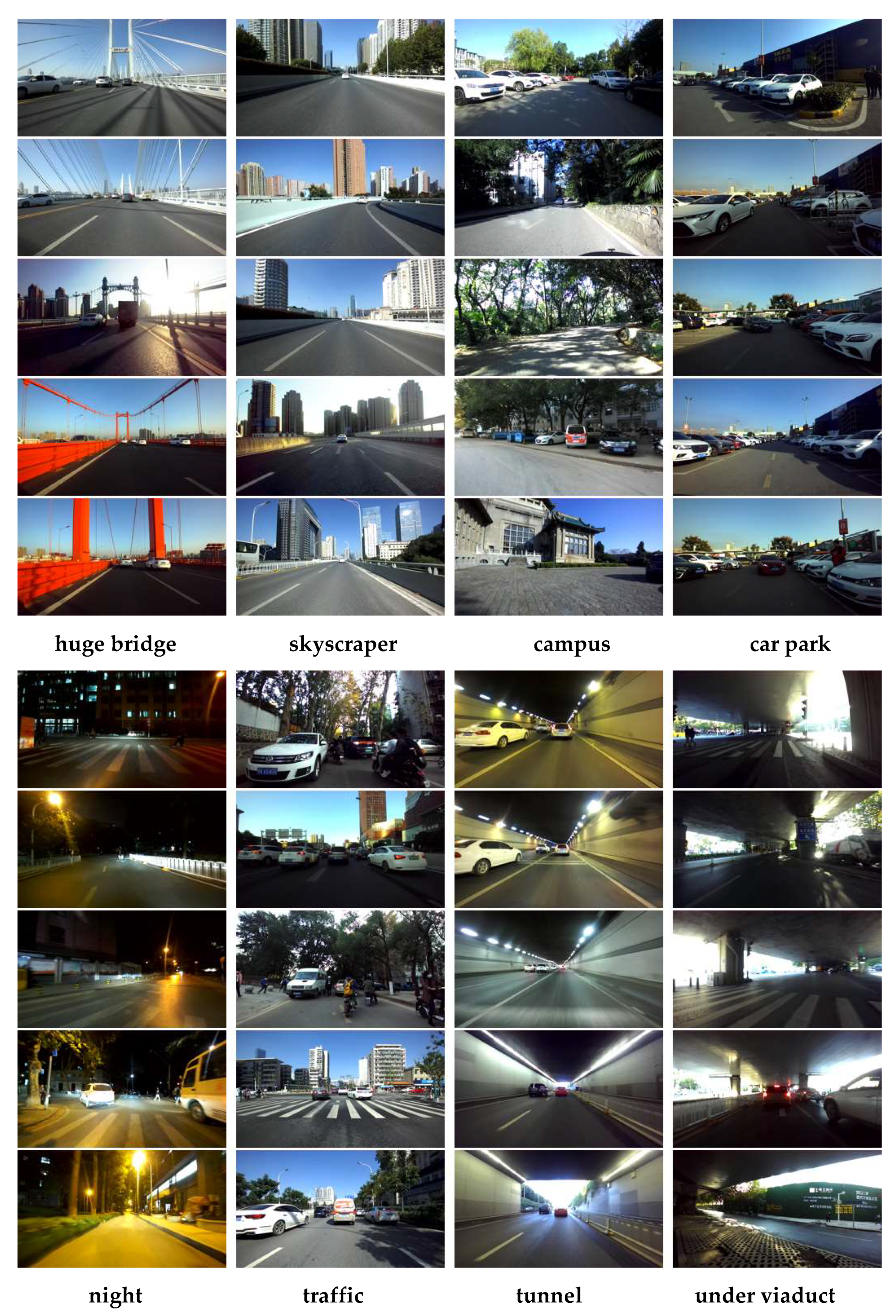
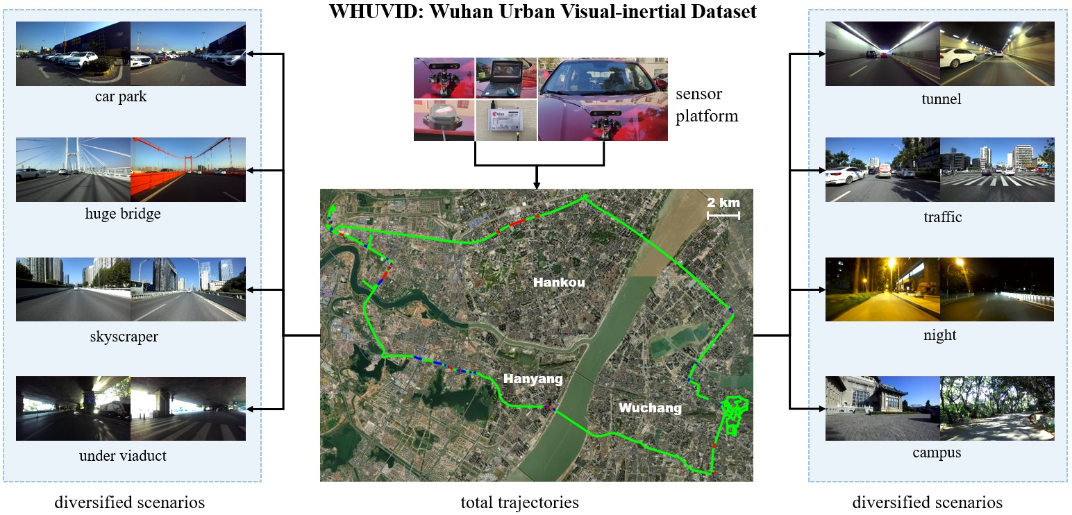
- We propose WHUVID, the latest and largest calibrated and synchronized visual-inertial dataset collected from Chinese urban scenarios with abundant scenes not previously included, along with high-quality recordings and accurate ground truth.
- We present a brief review of numerous previously published datasets and conduct a detailed evaluation and comparative experiments between some of them and WHUVID, proposing some original evaluation metrics.
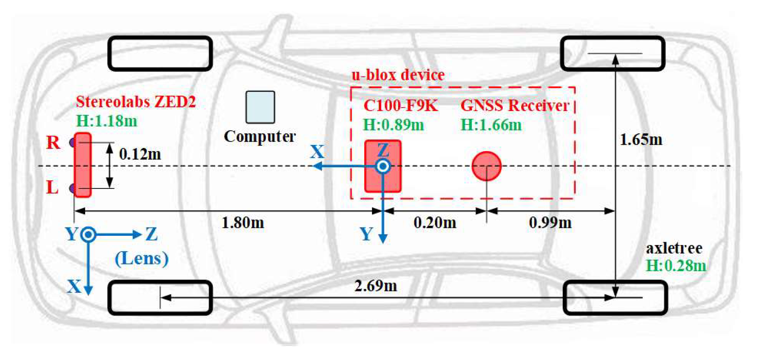
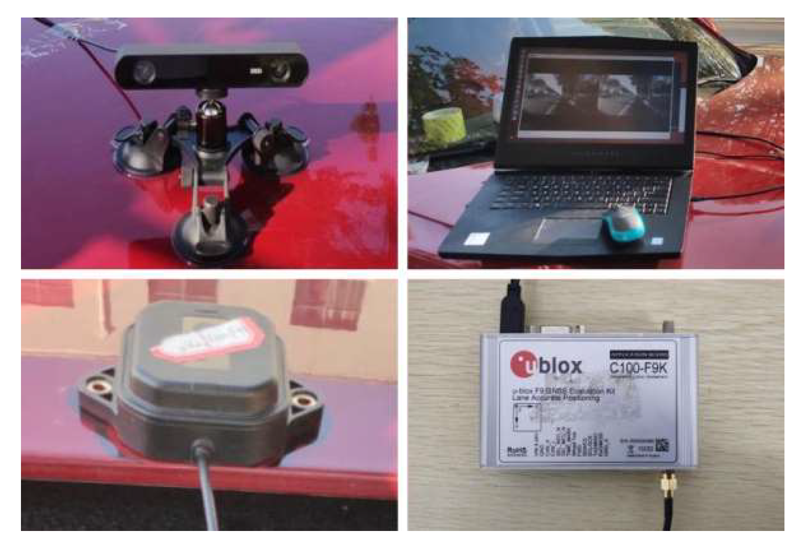
2. Sensor Setup
- A Stereolabs ZED2 integrated VI sensor with stereo lenses (1/3” 4MP CMOS, 2688 × 1520 pixels with each pixel of size 2 × 2 microns, electronic synchronized rolling shutter, baseline: 120 mm, focal length: 2.12 mm, field of view (FOV): 110° horiz. 70° vert.) and a consumer-grade built-in IMU (motion measurement with 6-DOF @ 400 Hz ± 0.4% error, magnetometer with 3-DOF @ 50 Hz ± 1300 µT);
- A u-blox GNSS-IMU navigation device (184-channel u-blox F9 engine; supporting GPS, GLONASS, BeiDou, Galileo, SBAS, and QZSS; position accuracy < 0.2 m + 1 ppm CEP with real-time kinematic (RTK); and data-update rate up to 30 Hz, with a built-in IMU for a GNSS-denied environment) with a GNSS receiver and a C100-F9K integrated module (IMU inside).
3. Dataset
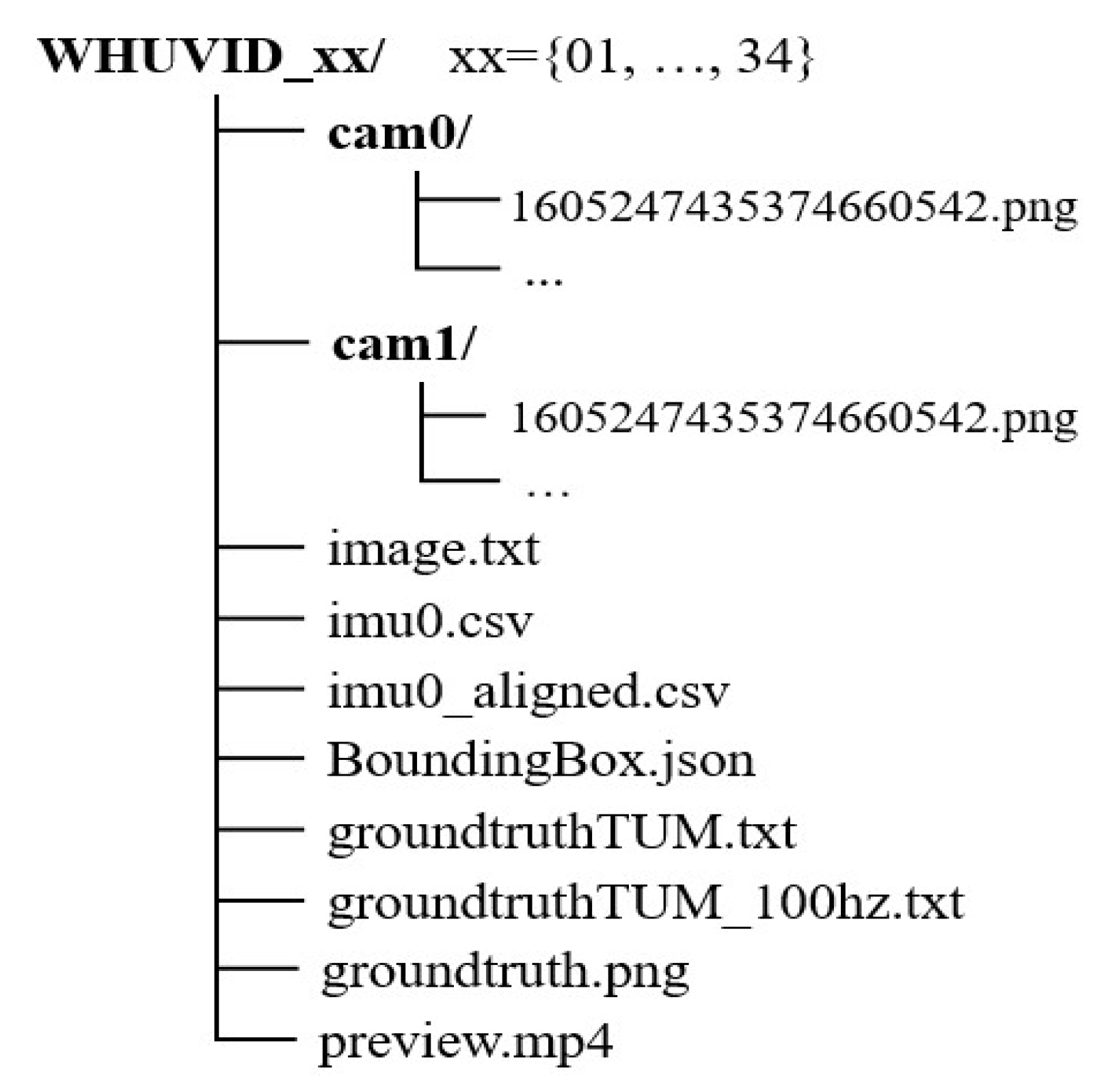
3.1. Data Description
3.1.1. Image and IMU
3.1.2. Ground Truth
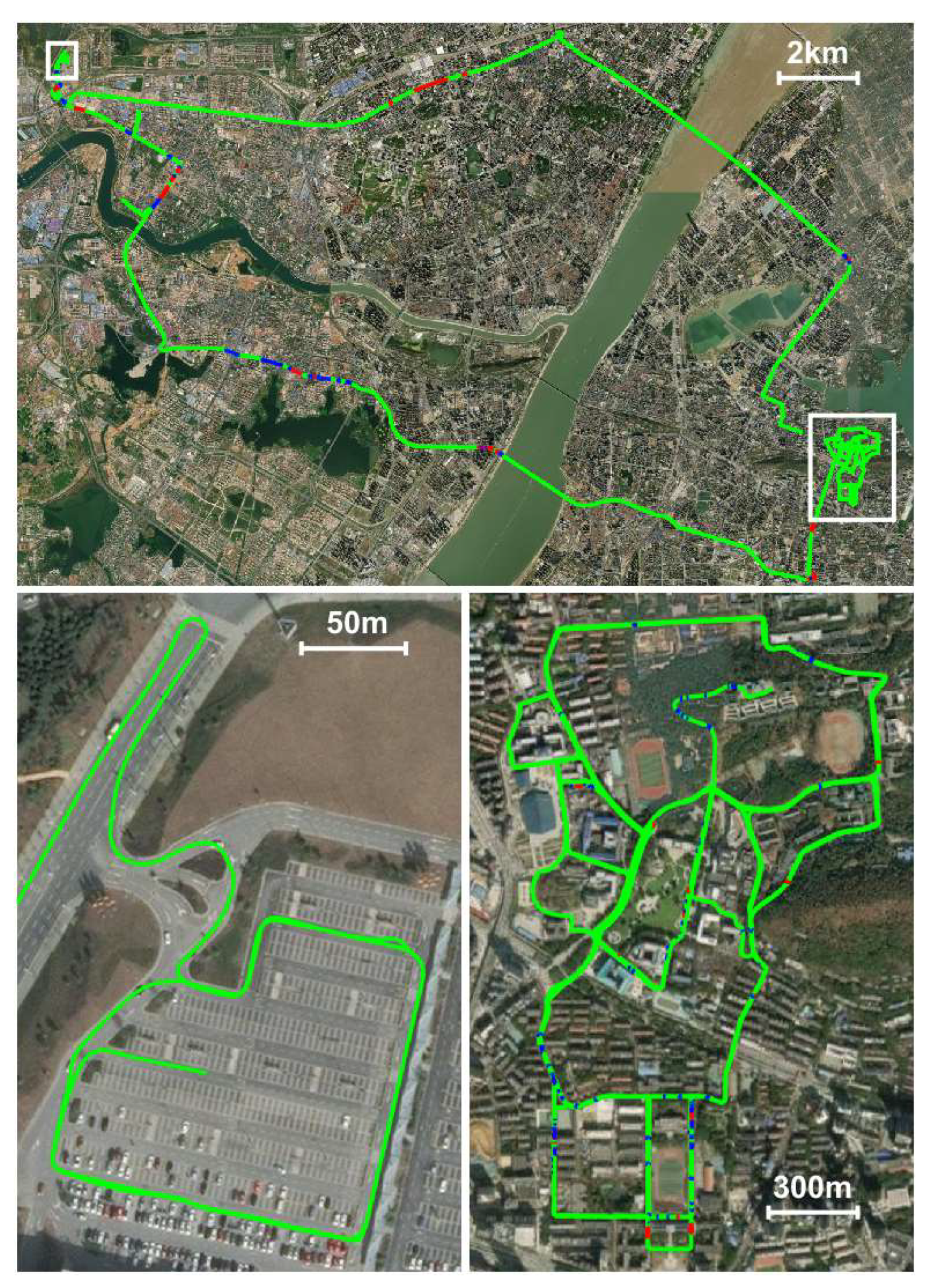
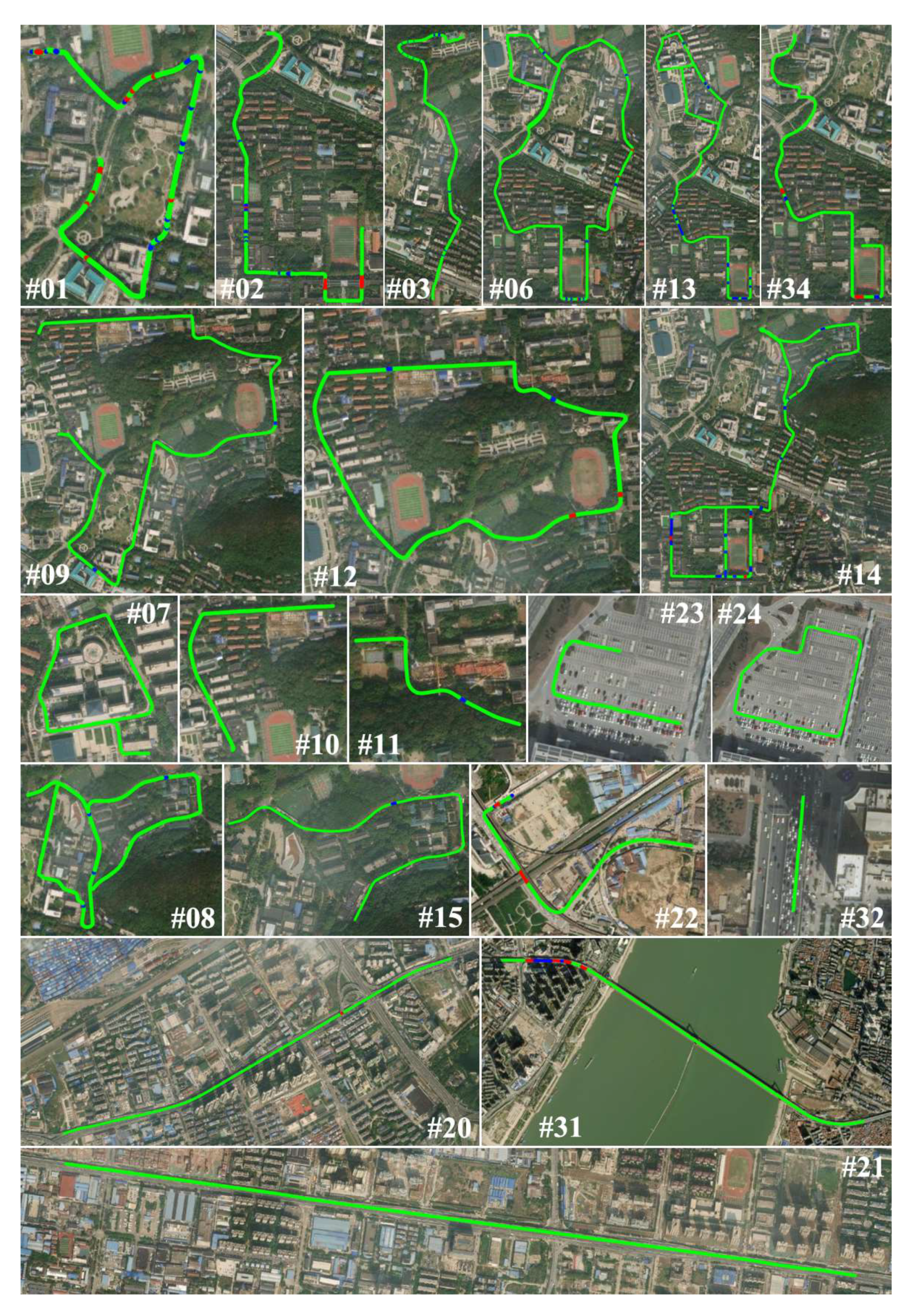
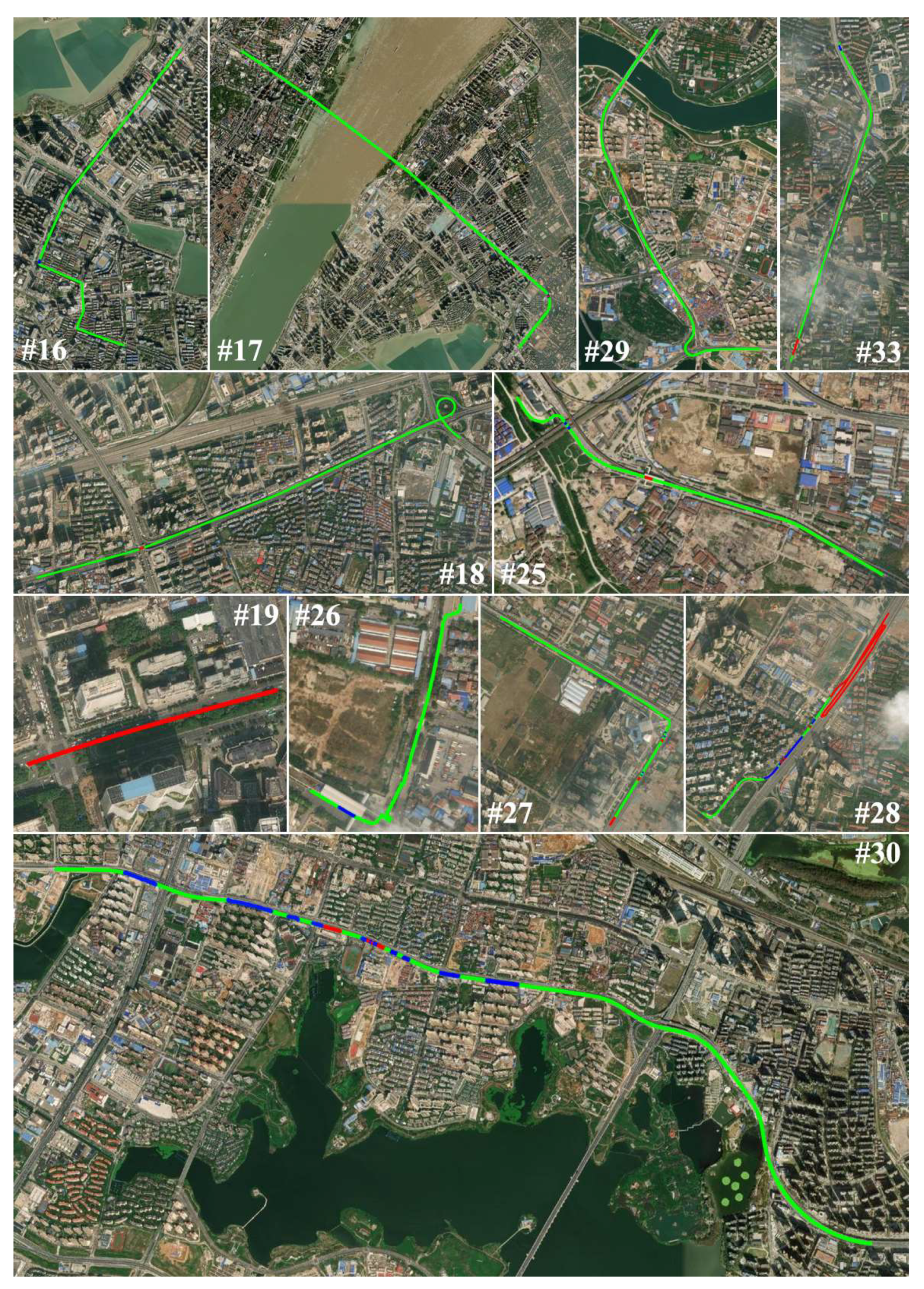
3.1.3. Sequences
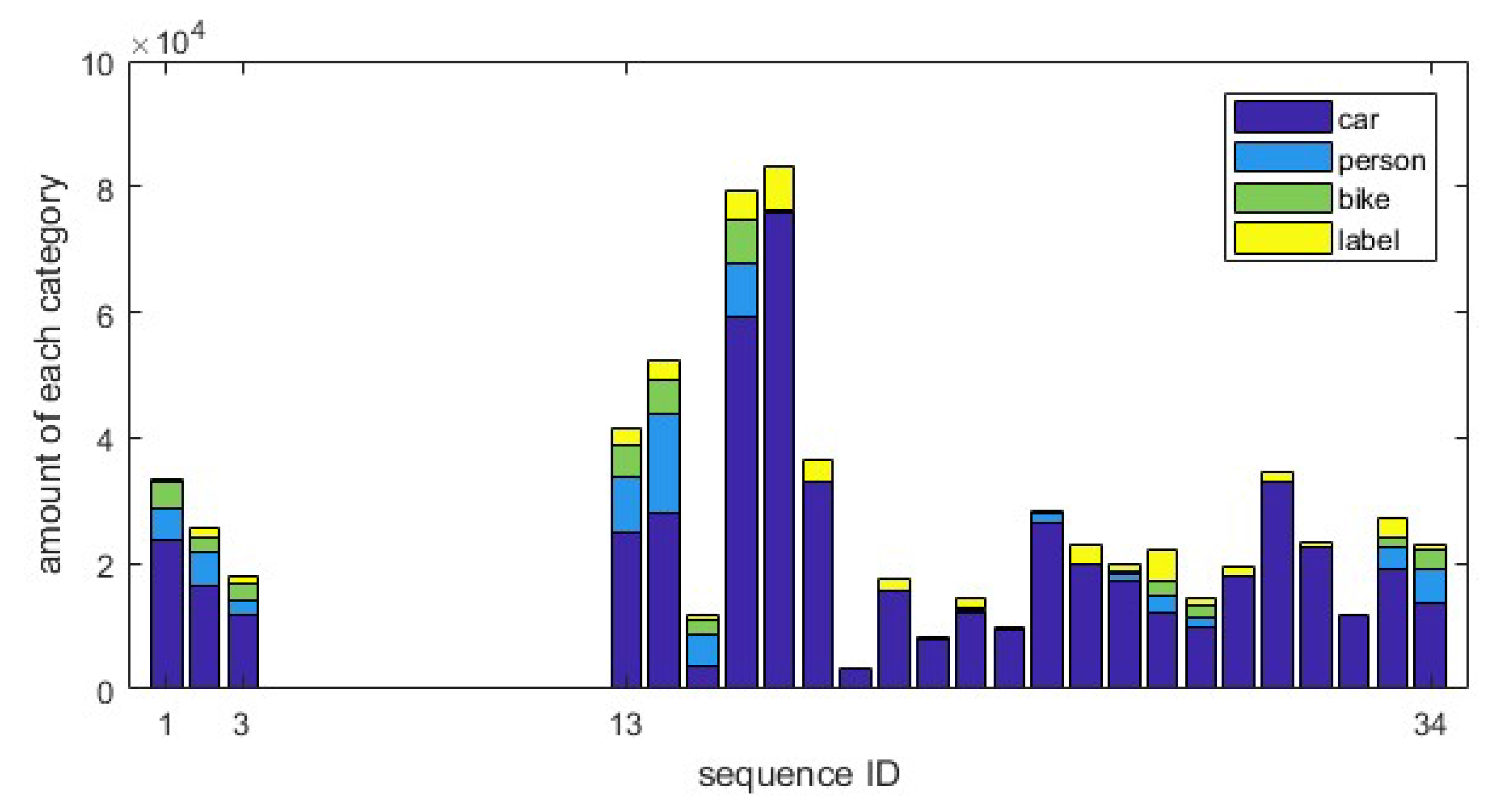
3.2. Annotations
4. Calibration and Synchronization
4.1. Stereolabs ZED2 Calibration
4.1.1. IMU
4.1.2. Stereo
4.1.3. Visual-IMU
4.2. GNSS Interpolation and IMU Timestamp Alignment
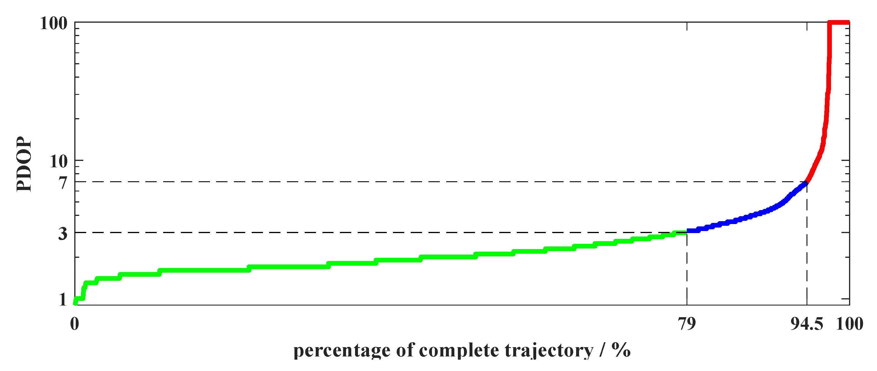
4.2.1. GNSS Interpolation
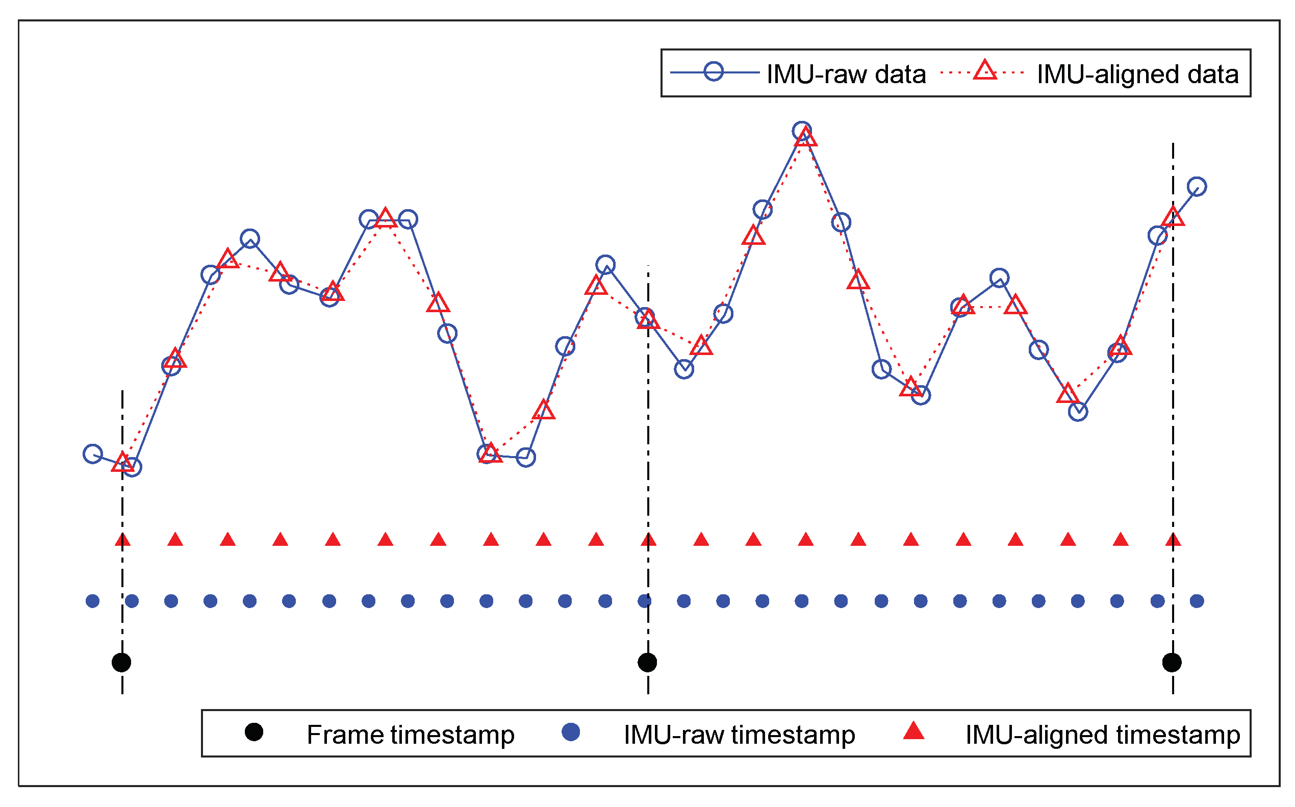
4.2.2. IMU Timestamp Alignment
5. Evaluation and Discussion
5.1. Evaluation Metric
5.2. Results and Discussion
6. Conclusions
Author Contributions
Funding
Data Availability Statement
Conflicts of Interest
Abbreviations
| WHUVID | Wuhan Urban Visual-inertial Dataset |
| VIO | visual-inertial odometry |
| SLAM | simultaneous localization and mapping |
| GNSS | Global Navigation Satellite System |
| IMU | inertial measurement unit |
| DOF | degree of freedom |
| VO | visual odometry |
| RGB-D | RGB-depth |
| UAV | unmanned aerial vehicle |
| AUV | autonomous underwater vehicles |
| ENU | east-north-up |
| PDOP | position dilution of precision |
| FOV | field of view |
| GPS | Global Positioning System |
| SBAS | Satellite-Based Augmentation System |
| QZSS | Quasi-Zenith Satellite System |
| CEP | circular error probable |
| RTK | real-time kinematic |
| SUV | sports utility vehicle |
| HDOP | horizontal component of position dilution of precision |
| VDOP | vertical component of position dilution of precision |
| DGPS | Differential Global Positioning System |
| DR | dead reckoning |
| APE | absolute pose error |
| RPE | relative pose error |
| NS | the number of subsegments |
| ATF | average tracked frames of subsegments |
| WAPE | weighted average of absolute pose error of subsequences |
| WRPE | weighted average of relative pose error of subsequences |
| TR | tracking rate of the whole section |
References
- Leung, K.Y.; Halpern, Y.; Barfoot, T.D.; Liu, H.H. The UTIAS multi-robot cooperative localization and mapping dataset. Int. J. Rob. Res. 2011, 30, 969–974. [Google Scholar] [CrossRef]
- Chen, D.M.; Baatz, G.; Köser, K.; Tsai, S.S.; Vedantham, R.; Pylvänäinen, T.; Roimela, K.; Chen, X.; Bach, J.; Pollefeys, M.; et al. City-scale landmark identification on mobile devices. In Proceedings of the CVPR 2011, Colorado Springs, CO, USA, 20–25 June 2011; pp. 737–744. [Google Scholar]
- Milford, M.J.; Wyeth, G.F. SeqSLAM: Visual route-based navigation for sunny summer days and stormy winter nights. In Proceedings of the 2012 IEEE International Conference on Robotics and Automation, Guangzhou, China, 11–14 December 2012; pp. 1643–1649. [Google Scholar]
- Guzmán, R.; Hayet, J.B.; Klette, R. Towards ubiquitous autonomous driving: The CCSAD dataset. In International Conference on Computer Analysis of Images and Patterns; Springer: Berlin/Heidelberg, Germany, 2015; pp. 582–593. [Google Scholar]
- Cordts, M.; Omran, M.; Ramos, S.; Rehfeld, T.; Enzweiler, M.; Benenson, R.; Franke, U.; Roth, S.; Schiele, B. The cityscapes dataset for semantic urban scene understanding. In Proceedings of the IEEE Conference on Computer Vision and Pattern Recognition, Las Vegas, NV, USA, 27–30 June 2016; pp. 3213–3223. [Google Scholar]
- Carlevaris-Bianco, N.; Ushani, A.K.; Eustice, R.M. University of Michigan North Campus long-term vision and lidar dataset. Int. J. Rob. Res. 2016, 35, 1023–1035. [Google Scholar] [CrossRef]
- Jung, H.; Oto, Y.; Mozos, O.M.; Iwashita, Y.; Kurazume, R. Multi-modal panoramic 3D outdoor datasets for place categorization. In Proceedings of the 2016 IEEE/RSJ International Conference on Intelligent Robots and Systems (IROS), Daejeon, Korea, 9–14 October 2016; pp. 4545–4550. [Google Scholar]
- Pandey, G.; McBride, J.R.; Eustice, R.M. Ford campus vision and lidar data set. Int. J. Rob. Res. 2011, 30, 1543–1552. [Google Scholar] [CrossRef]
- Geiger, A.; Lenz, P.; Stiller, C.; Urtasun, R. Vision meets robotics: The kitti dataset. Int. J. Rob. Res. 2013, 32, 1231–1237. [Google Scholar] [CrossRef] [Green Version]
- Geiger, A.; Lenz, P.; Urtasun, R. Are we ready for autonomous driving? The kitti vision benchmark suite. In Proceedings of the 2012 IEEE Conference on Computer Vision and Pattern Recognition, Providence, RI, USA, 16–21 June 2012; pp. 3354–3361. [Google Scholar]
- Sturm, J.; Engelhard, N.; Endres, F.; Burgard, W.; Cremers, D. A benchmark for the evaluation of RGB-D SLAM systems. In Proceedings of the 2012 IEEE/RSJ international conference on intelligent robots and systems, Faro, Portugal, 7–12 October 2012; pp. 573–580. [Google Scholar]
- Zhu, A.Z.; Thakur, D.; Özaslan, T.; Pfrommer, B.; Kumar, V.; Daniilidis, K. The multivehicle stereo event camera dataset: An event camera dataset for 3D perception. IEEE Robot. Autom. Lett. 2018, 3, 2032–2039. [Google Scholar] [CrossRef] [Green Version]
- Chebrolu, N.; Lottes, P.; Schaefer, A.; Winterhalter, W.; Burgard, W.; Stachniss, C. Agricultural robot dataset for plant classification, localization and mapping on sugar beet fields. Int. J. Rob. Res. 2017, 36, 1045–1052. [Google Scholar] [CrossRef] [Green Version]
- Hewitt, R.A.; Boukas, E.; Azkarate, M.; Pagnamenta, M.; Marshall, J.A.; Gasteratos, A.; Visentin, G. The Katwijk beach planetary rover dataset. Int. J. Rob. Res. 2018, 37, 3–12. [Google Scholar] [CrossRef] [Green Version]
- Burri, M.; Nikolic, J.; Gohl, P.; Schneider, T.; Rehder, J.; Omari, S.; Achtelik, M.W.; Siegwart, R. The EuRoC micro aerial vehicle datasets. Int. J. Rob. Res. 2016, 35, 1157–1163. [Google Scholar] [CrossRef]
- Majdik, A.L.; Till, C.; Scaramuzza, D. The Zurich urban micro aerial vehicle dataset. Int. J. Rob. Res. 2017, 36, 269–273. [Google Scholar] [CrossRef] [Green Version]
- Ferrera, M.; Creuze, V.; Moras, J.; Trouvé-Peloux, P. AQUALOC: An underwater dataset for visual–inertial–pressure localization. Int. J. Rob. Res. 2019, 38, 1549–1559. [Google Scholar] [CrossRef]
- Mallios, A.; Vidal, E.; Campos, R.; Carreras, M. Underwater caves sonar data set. Int. J. Rob. Res. 2017, 36, 1247–1251. [Google Scholar] [CrossRef]
- Bender, A.; Williams, S.B.; Pizarro, O. Autonomous exploration of large-scale benthic environments. In Proceedings of the 2013 IEEE International Conference on Robotics and Automation, Karlsruhe, Germany, 6–10 May 2013; pp. 390–396. [Google Scholar]
- Golodetz, S.; Cavallari, T.; Lord, N.A.; Prisacariu, V.A.; Murray, D.W.; Torr, P.H. Collaborative large-scale dense 3d reconstruction with online inter-agent pose optimisation. IEEE Trans. Vis. Comput. Graph. 2018, 24, 2895–2905. [Google Scholar] [CrossRef] [PubMed] [Green Version]
- Schubert, D.; Goll, T.; Demmel, N.; Usenko, V.; Stückler, J.; Cremers, D. The TUM VI benchmark for evaluating visual-inertial odometry. In Proceedings of the 2018 IEEE/RSJ International Conference on Intelligent Robots and Systems (IROS), Madrid, Spain, 1–5 October 2018; pp. 1680–1687. [Google Scholar]
- Choi, Y.; Kim, N.; Hwang, S.; Park, K.; Yoon, J.S.; An, K.; Kweon, I.S. KAIST multi-spectral day/night data set for autonomous and assisted driving. IEEE Trans. Intell. Transp. Syst. 2018, 19, 934–948. [Google Scholar] [CrossRef]
- Jeong, J.; Cho, Y.; Shin, Y.S.; Roh, H.; Kim, A. Complex urban dataset with multi-level sensors from highly diverse urban environments. Int. J. Rob. Res. 2019, 38, 642–657. [Google Scholar] [CrossRef] [Green Version]
- Fraundorfer, F.; Scaramuzza, D. Visual odometry: Part i: The first 30 years and fundamentals. IEEE Robot. Autom. Mag. 2011, 18, 80–92. [Google Scholar]
- Fraundorfer, F.; Scaramuzza, D. Visual odometry: Part ii: Matching, robustness, optimization, and applications. IEEE Robot. Autom. Mag. 2012, 19, 78–90. [Google Scholar] [CrossRef] [Green Version]
- Aqel, M.O.; Marhaban, M.H.; Saripan, M.I.; Ismail, N.B. Review of visual odometry: Types, approaches, challenges, and applications. Springerplus 2016, 5, 1897. [Google Scholar] [CrossRef] [Green Version]
- Durrant-Whyte, H.; Bailey, T. Simultaneous localization and mapping: Part I. IEEE Robot. Autom. Mag. 2006, 13, 99–110. [Google Scholar] [CrossRef] [Green Version]
- Bailey, T.; Durrant-Whyte, H. Simultaneous localization and mapping (SLAM): Part II. IEEE Robot. Autom. Mag. 2006, 13, 108–117. [Google Scholar] [CrossRef] [Green Version]
- Cadena, C.; Carlone, L.; Carrillo, H.; Latif, Y.; Scaramuzza, D.; Neira, J.; Reid, I.; Leonard, J.J. Past, present, and future of simultaneous localization and mapping: Toward the robust-perception age. IEEE Trans. Robot. 2016, 32, 1309–1332. [Google Scholar] [CrossRef] [Green Version]
- Bochkovskiy, A.; Wang, C.Y.; Liao, H.Y.M. Yolov4: Optimal speed and accuracy of object detection. arXiv 2020, arXiv:2004.10934. [Google Scholar]
- Mur-Artal, R.; Montiel, J.M.M.; Tardos, J.D. ORB-SLAM: A versatile and accurate monocular SLAM system. IEEE Trans. Robot. 2015, 31, 1147–1163. [Google Scholar] [CrossRef] [Green Version]
- Mur-Artal, R.; Tardós, J.D. Orb-slam2: An open-source slam system for monocular, stereo, and rgb-d cameras. IEEE Trans. Robot. 2017, 33, 1255–1262. [Google Scholar] [CrossRef] [Green Version]
- Qin, T.; Li, P.; Shen, S. Vins-mono: A robust and versatile monocular visual-inertial state estimator. IEEE Trans. Robot. 2018, 34, 1004–1020. [Google Scholar] [CrossRef] [Green Version]
- Qin, T.; Shen, S. Online temporal calibration for monocular visual-inertial systems. In Proceedings of the 2018 IEEE/RSJ International Conference on Intelligent Robots and Systems (IROS), Madrid, Spain, 1–5 October 2018; pp. 3662–3669. [Google Scholar]
- Blanco-Claraco, J.L.; Moreno-Duenas, F.A.; González-Jiménez, J. The Málaga urban dataset: High-rate stereo and LiDAR in a realistic urban scenario. Int. J. Rob. Res. 2014, 33, 207–214. [Google Scholar] [CrossRef] [Green Version]
- Maddern, W.; Pascoe, G.; Linegar, C.; Newman, P. 1 year, 1000 km: The Oxford RobotCar dataset. Int. J. Rob. Res. 2017, 36, 3–15. [Google Scholar] [CrossRef]
- Walter, L.; Oliver, B.; Oliver, B.; Karol, P.; Pierre, Y.; Max, P. A Platform-Agnostic Camera and Sensor Capture API for the ZED Stereo Camera Family. 2020. Available online: https://github.com/stereolabs/zed-open-capture (accessed on 22 May 2018).
- Grafarend, E. The optimal universal transverse Mercator projection. In Geodetic Theory Today; Springer: Berlin/Heidelberg, Germany, 1995; p. 51. [Google Scholar]
- Woodman, O.J. An introduction to inertial navigation. In Technical Report UCAM-CL-TR-696; University of Cambridge, Computer Laboratory: Cambridge, UK, 2007. [Google Scholar] [CrossRef]
- Zhang, Z. Flexible camera calibration by viewing a plane from unknown orientations. In Proceedings of the seventh IEEE international conference on computer vision, Washington, DC, USA, 20–25 September 1999; Volume 1, pp. 666–673. [Google Scholar]
- Rehder, J.; Nikolic, J.; Schneider, T.; Hinzmann, T.; Siegwart, R. Extending kalibr: Calibrating the extrinsics of multiple IMUs and of individual axes. In Proceedings of the 2016 IEEE International Conference on Robotics and Automation (ICRA), Stockholm, Sweden, 16–21 May 2016; pp. 4304–4311. [Google Scholar]
- Furgale, P.; Rehder, J.; Siegwart, R. Unified temporal and spatial calibration for multi-sensor systems. In Proceedings of the 2013 IEEE/RSJ International Conference on Intelligent Robots and Systems, Tokyo, Japan, 3–7 November 2013; pp. 1280–1286. [Google Scholar]
- Furgale, P.; Barfoot, T.D.; Sibley, G. Continuous-time batch estimation using temporal basis functions. In Proceedings of the 2012 IEEE International Conference on Robotics and Automation, Guangzhou, China, 11–14 December 2012; pp. 2088–2095. [Google Scholar]
- Maye, J.; Furgale, P.; Siegwart, R. Self-supervised calibration for robotic systems. In Proceedings of the 2013 IEEE Intelligent Vehicles Symposium (IV), Gold Coast City, Australia, 23–26 June 2013; pp. 473–480. [Google Scholar]
- Oth, L.; Furgale, P.; Kneip, L.; Siegwart, R. Rolling shutter camera calibration. In Proceedings of the IEEE Conference on Computer Vision and Pattern Recognition, Portland, OR, USA, 23–28 June 2013; pp. 1360–1367. [Google Scholar]
- Grupp, M. Evo: Python Package for the Evaluation of Odometry and SLAM. 2017. Available online: https://github.com/MichaelGrupp/evo (accessed on 14 September 2017).
- Klein, G.; Murray, D. Parallel tracking and mapping for small AR workspaces. In Proceedings of the 2007 6th IEEE and ACM International Symposium on Mixed and Augmented Reality, Nara, Japan, 13–16 November 2007; pp. 225–234. [Google Scholar]
- Davison, A.J.; Reid, I.D.; Molton, N.D.; Stasse, O. MonoSLAM: Real-time single camera SLAM. IEEE Trans. Pattern Anal. Mach. Intell. 2007, 29, 1052–1067. [Google Scholar] [CrossRef] [Green Version]
- Newcombe, R.A.; Lovegrove, S.J.; Davison, A.J. DTAM: Dense tracking and mapping in real-time. In Proceedings of the 2011 IEEE international conference on computer vision, Barcelona, Spain, 6–13 November 2011; pp. 2320–2327. [Google Scholar]
- Kerl, C.; Sturm, J.; Cremers, D. Dense visual SLAM for RGB-D cameras. In Proceedings of the 2013 IEEE/RSJ International Conference on Intelligent Robots and Systems, Tokyo, Japan, 3–7 November 2013; pp. 2100–2106. [Google Scholar]
- Engel, J.; Schöps, T.; Cremers, D. LSD-SLAM: Large-scale direct monocular SLAM. In European Conference on Computer Vision; Springer: Berlin/Heidelberg, Germany, 2014; pp. 834–849. [Google Scholar]
- Forster, C.; Pizzoli, M.; Scaramuzza, D. SVO: Fast semi-direct monocular visual odometry. In Proceedings of the 2014 IEEE international conference on robotics and automation (ICRA), Hong Kong, China, 31 May–7 June 2014; pp. 15–22. [Google Scholar]
- Leutenegger, S.; Lynen, S.; Bosse, M.; Siegwart, R.; Furgale, P. Keyframe-based visual–inertial odometry using nonlinear optimization. Int. J. Rob. Res. 2015, 34, 314–334. [Google Scholar] [CrossRef] [Green Version]
- Bloesch, M.; Omari, S.; Hutter, M.; Siegwart, R. Robust visual inertial odometry using a direct EKF-based approach. In Proceedings of the 2015 IEEE/RSJ international conference on intelligent robots and systems (IROS), Hamburg, Germany, 28 September–3 October 2015; pp. 298–304. [Google Scholar]
- Zihao Zhu, A.; Atanasov, N.; Daniilidis, K. Event-based visual inertial odometry. In Proceedings of the IEEE Conference on Computer Vision and Pattern Recognition, Honolulu, HI, USA, 21–26 July 2017; pp. 5391–5399. [Google Scholar]
- Yu, C.; Liu, Z.; Liu, X.J.; Xie, F.; Yang, Y.; Wei, Q.; Fei, Q. DS-SLAM: A semantic visual SLAM towards dynamic environments. In Proceedings of the 2018 IEEE/RSJ International Conference on Intelligent Robots and Systems (IROS), Madrid, Spain, 1–5 October 2018; pp. 1168–1174. [Google Scholar]
- Bescos, B.; Fácil, J.M.; Civera, J.; Neira, J. DynaSLAM: Tracking, mapping, and inpainting in dynamic scenes. IEEE Robot. Autom. Lett. 2018, 3, 4076–4083. [Google Scholar] [CrossRef] [Green Version]
- Henein, M.; Zhang, J.; Mahony, R.; Ila, V. Dynamic SLAM: The need for speed. In Proceedings of the 2020 IEEE International Conference on Robotics and Automation (ICRA), Paris, France, 31 May–31 August 2020; pp. 2123–2129. [Google Scholar]
- Nair, G.B.; Daga, S.; Sajnani, R.; Ramesh, A.; Ansari, J.A.; Jatavallabhula, K.M.; Krishna, K.M. Multi-object monocular SLAM for dynamic environments. In Proceedings of the 2020 IEEE Intelligent Vehicles Symposium (IV), Las Vegas, NV, USA, 19 October–13 November 2020; pp. 651–657. [Google Scholar]
- Zhang, J.; Henein, M.; Mahony, R.; Ila, V. VDO-SLAM: A visual dynamic object-aware SLAM system. arXiv 2020, arXiv:2005.11052. [Google Scholar]
- Campos, C.; Elvira, R.; Rodríguez, J.J.G.; Montiel, J.M.; Tardós, J.D. Orb-slam3: An accurate open-source library for visual, visual–inertial, and multimap slam. IEEE Trans. Robot. 2021, 37, 1874–1890. [Google Scholar] [CrossRef]


| Dataset | Release Year | Position | #Seq | #Frame | Dur/s | Len/km | Avg Spd/(m/s) | Camera Parameter | #Category | #Label | GT Quality |
|---|---|---|---|---|---|---|---|---|---|---|---|
| FORD [8] | 2011 | Dearborn, USA | 2 | 7 k | 938 | 5.4 | 5.8 | omni × 6 RGB 1600 × 600 @ 8 fps | None | None | 6-DOF |
| KITTI [9,10] | 2013 | Karlsruhe, Germany | 22 | 41 k | 4517 | 39.2 | 8.7 | stereo RGB 1241 × 376 @ 10 fps | 5 | — | 6-DOF |
| Malaga [35] | 2014 | Malaga, Spain | 15 | 113 k | 5655 | 36.8 | 6.5 | stereo RGB 1024 × 768 @ 20 fps | None | None | 3-DOF |
| Oxford 1 [36] | 2016 | Oxford, UK | 1 | 35 k | 2455 | 9.3 | 3.8 | stereo RGB 1280 × 960 @ 16 fps | None | None | 6-DOF |
| EuRoC 2 [15] | 2016 | Zurich, Switzerland | 11 | 27 k | 1373 | 0.89 | 0.65 | mono GRAY 752 × 480 @ 20 fps | None | None | 6-DOF |
| MVSEC [12] | 2018 | West Philly, USA | 5 | 37 k | 1813 | 9.6 | 5.3 | stereo GRAY 752 × 480 @ 20 fps | None | None | 6-DOF |
| WHUVID | 2021 | Wuhan, China | 34 | 336 k | 11,285 | 82.0 | 7.2 | stereo RGB 1280 × 720 @ 30 fps | 4 | 681 k | 6-DOF |
| Id | Scene 1 | Period | Duration/s Length/m | #Frames | Speed/(m/s) | #Labels | Dynamic 2 | IMU 3 | GNSS | GNSS Quality | ||||
|---|---|---|---|---|---|---|---|---|---|---|---|---|---|---|
| Max | Mid | Mean | Min | Num | Ratio/% | |||||||||
| 01 | campus | p.m. | 301, 1511 | 9006 | 12.1 | 4.9 | 5.0 | 0 | 33,461 | 3.7 | 5.0 | Y | Y | 4.2 |
| 02 | campus | p.m. | 288, 1610 | 8631 | 9.9 | 5.4 | 5.6 | 1.4 | 25,635 | 2.8 | 8.0 | Y | Y | 2.7 |
| 03 | campus | p.m. | 283, 1531 | 8486 | 10.4 | 5.5 | 5.4 | 0.4 | 18,021 | 2.0 | 3.2 | Y | Y | 2.7 |
| 04 | campus | p.m. | 172, 1100 | 5104 | 11.5 | 8.0 | 6.4 | 1.5 | — | — | — | N | PD | 1.4 |
| 05 | campus | sunset | 1188, 4775 | 35,576 | 10.0 | 3.7 | 4.0 | 0 | — | — | — | N | PD | 2.4 |
| 06 | campus | night | 822, 4775 | 24,618 | 12.9 | 5.8 | 5.8 | 0.1 | — | — | — | Y | Y | 1.9 |
| 07 | campus | night | 166, 790 | 4914 | 9.3 | 4.5 | 4.8 | 0 | — | — | — | Y | Y | 1.8 |
| 08 | campus | night | 403, 2474 | 11,825 | 11.3 | 6.4 | 6.1 | 1.1 | — | — | — | N | Y | 2.2 |
| 09 | campus | night | 490, 3221 | 14,655 | 10.9 | 6.9 | 6.6 | 1.2 | — | — | — | Y | Y | 2.8 |
| 10 | campus | night | 131, 887 | 3866 | 9.4 | 7.1 | 6.8 | 0.8 | — | — | — | Y | Y | 2.8 |
| 11 | campus | night | 58, 352 | 1727 | 8.4 | 6.3 | 6.1 | 1.4 | — | — | — | Y | Y | 2.9 |
| 12 | campus | night | 495, 3028 | 14,784 | 10.4 | 6.3 | 6.1 | 1.1 | — | — | — | Y | Y | 2.3 |
| 13 | campus | a.m. | 569, 3891 | 16,985 | 11.4 | 6.9 | 6.8 | 2.1 | 41,410 | 2.3 | 4.1 | Y | Y | 2.0 |
| 14 | campus | a.m. | 797, 4531 | 23,811 | 11.3 | 5.7 | 5.7 | 0 | 52,373 | 2.0 | 4.0 | Y | Y | 2.7 |
| 15 | campus | a.m. | 248, 980 | 7354 | 8.8 | 5.1 | 5.4 | 0 | 11,785 | 1.5 | 2.7 | Y | Y | 2.0 |
| 16 | urban-RD | midday | 608, 4165 | 18,070 | 17.1 | 5.8 | 6.9 | 0 | 79,265 | 4.1 | 8.8 | Y | Y | 1.9 |
| 17 | urban-BG | midday | 621, 8028 | 18,420 | 18.9 | 13.5 | 12.9 | 0 | 83,138 | 4.1 | 8.6 | Y | Y | 1.7 |
| 18 | urban-RD | midday | 267, 2925 | 8000 | 17.3 | 10.6 | 11.0 | 2.8 | 36,472 | 4.1 | 7.9 | Y | Y | 1.9 |
| 19 | urban-TN | midday | 35, 361 | 1042 | 13.8 | 10.3 | 10.3 | 7.1 | 3251 | 3.1 | 6.6 | Y | Y | 100 |
| 20 | urban-RD | midday | 143, 2112 | 4003 | 17.9 | 14.5 | 14.8 | 9.9 | 17,549 | 3.9 | 5.4 | Y | Y | 1.6 |
| 21 | urban-RD | midday | 164, 2902 | 4903 | 23.1 | 17.4 | 17.7 | 10.6 | 8300 | 1.6 | 2.3 | Y | Y | 1.4 |
| 22 | urban-RD | midday | 137, 1137 | 4107 | 13.6 | 9.9 | 8.3 | 0 | 14,414 | 3.1 | 7.6 | Y | Y | 1.6 |
| 23 | urban-CP | p.m. | 80, 206 | 2381 | 5.4 | 2.8 | 2.6 | 0 | 9853 | 4.1 | 15.6 | Y | Y | 1.7 |
| 24 | urban-CP | p.m. | 217, 486 | 6493 | 5.7 | 2.1 | 2.2 | 0 | 28,330 | 4.2 | 12.1 | Y | Y | 1.7 |
| 25 | urban-RD | p.m. | 258, 1696 | 7713 | 16.9 | 5.0 | 6.6 | 0 | 23,055 | 2.6 | 8.0 | Y | Y | 1.6 |
| 26 | urban-RD | p.m. | 219, 585 | 6478 | 9.7 | 1.2 | 2.7 | 0 | 19,727 | 2.9 | 9.5 | Y | Y | 2.1 |
| 27 | urban-RD | p.m. | 239, 1661 | 7154 | 16.0 | 6.7 | 6.9 | 0 | 22,279 | 2.4 | 3.7 | Y | Y | 2.0 |
| 28 | urban-RD | p.m. | 321, 1737 | 9565 | 14.5 | 5.5 | 5.4 | 0 | 14,305 | 1.4 | 4.1 | Y | Y | 100 |
| 29 | urban-RD | sunset | 302, 4437 | 9045 | 23.2 | 14.8 | 14.7 | 5.5 | 19,372 | 2.0 | 2.5 | Y | Y | 1.6 |
| 30 | urban-RD | sunset | 405, 5936 | 12,027 | 21.6 | 14.7 | 14.7 | 5.9 | 34,555 | 2.7 | 4.2 | Y | Y | 2.8 |
| 31 | urban-BG | sunset | 219, 3942 | 6480 | 20.2 | 15.6 | 18.0 | 12.7 | 23,206 | 3.5 | 4.3 | Y | Y | 1.6 |
| 32 | urban-RD | sunset | 72, 108 | 1864 | 2.6 | 1.5 | 1.5 | 0.5 | 11,719 | 6.3 | 24.8 | Y | Y | 1.7 |
| 33 | urban-RD | sunset | 265, 2187 | 7945 | 17.3 | 11.0 | 8.3 | 0 | 27,207 | 3.0 | 6.4 | Y | Y | 2.4 |
| 34 | campus | sunset | 302, 1944 | 9043 | 10.3 | 6.7 | 6.4 | 0.9 | 23,027 | 2.4 | 6.0 | Y | Y | 2.4 |
| Class | Car | Person | Bike | Label | In Total |
|---|---|---|---|---|---|
| AP or mAP/% | 97.47 | 91.35 | 94.77 | 96.41 | 95.00 |
| Category | Manually | All | ||
|---|---|---|---|---|
| Number | Percent/% | Number | Percent/% | |
| car | 5396 | 72.09 | 528,048 | 77.46 |
| person | 761 | 10.17 | 67,885 | 9.96 |
| bike | 474 | 6.33 | 39,505 | 5.79 |
| label | 854 | 11.41 | 46,271 | 6.79 |
| In total | 7485 | 100 | 681,709 | 100 |
| IMU | ||
| accelerometer_noise_density | 2.499898 × 10⁻² | |
| accelerometer_random_walk | 3.833771 × 10⁻⁴ | |
| gyroscope_noise_density | 2.143949 × 10⁻³ | |
| gyroscope_random_walk | 1.716940 × 10⁻⁵ | |
| Stereo | ||
| cam0 | intrinsic 1 | 526.83, 529.30, 638.38, 362.98 |
| distortion 2 | −0.0615, 0.0148, −0.0000423, −0.00470 | |
| cam1 | intrinsic | 524.90, 529.95, 656.21, 343.63 |
| distortion | −0.0385, −0.00112, 0.000166, −0.00572 | |
| baseline | rotation 3 | −0.00355, 0.00117, 0.000204, 1.0 |
| translation | −0.120, −0.000202, 0.00207 | |
| Visual-IMU | ||
| T_ic (cam0 to imu) | rotation matrix | [0.00815, 1.0, 0.00726; 1.0, −0.00797, −0.0248; −0.0247, 0.00746, −1.0] |
| translation | 0.00184, −0.0226, −0.0225 | |
| Dataset | Monocular | Stereo | Visual-Inertial | |||||||||||||
|---|---|---|---|---|---|---|---|---|---|---|---|---|---|---|---|---|
| Name | Seq Id | NS | ATF | WAPE | WRPE | TR/% | NS | ATF | WAPE | WRPE | TR/% | NS | ATF | WAPE | WRPE | TR/% |
| FORD | 1 | 9 | 276 | 4.78 | 4.30 | 81.3 | - | - | - | - | - | - | - | - | - | - |
| 2 | 6 | 481 | 61.47 | 7.04 | 61.1 | - | - | - | - | - | - | - | - | - | - | |
| Oxford | 9 | 3657 | 19.62 | 2.27 | 93.1 | 15 | 2312 | 39.77 | 0.50 | 98.1 | - | - | - | - | - | |
| MVSEC | day 1 | 2 | 2220 | 6.12 | 2.03 | 84.8 | 3 | 1684 | 6.05 | 0.60 | 96.5 | 3 | 1701 | 23.78 | 0.42 | 97.4 |
| day 2 | 1 | 12,069 | 6.33 | 2.98 | 92.4 | 1 | 13,063 | 25.01 | 1.51 | 100 | 7 | 1638 | 61.59 | 0.47 | 87.7 | |
| EuRoC | MH01 | - | - | - | - | - | - | - | - | - | - | 1 | 3682 | 0.13 | 0.0030 | 100 |
| MH02 | - | - | - | - | - | - | - | - | - | - | 1 | 3038 | 0.13 | 0.0024 | 99.9 | |
| MH03 | - | - | - | - | - | - | - | - | - | - | 1 | 2698 | 0.17 | 0.0049 | 99.9 | |
| MH04 | - | - | - | - | - | - | - | - | - | - | 1 | 2031 | 0.30 | 0.0046 | 99.9 | |
| MH05 | - | - | - | - | - | - | - | - | - | - | 1 | 2271 | 0.30 | 0.0051 | 99.9 | |
| KITTI | 00 | 1 | 4538 | 6.67 | 0.16 | 99.9 | 1 | 4541 | 0.86 | 0.02 | 100 | - | - | - | - | - |
| 01 | 1 | 1062 | 458.9 | 10.53 | 96.5 | 1 | 1101 | 8.68 | 0.04 | 100 | - | - | - | - | - | |
| 02 | 1 | 4658 | 22.29 | 0.22 | 99.9 | 1 | 4661 | 5.42 | 0.02 | 100 | - | - | - | - | - | |
| 03 | 1 | 798 | 0.66 | 0.05 | 99.6 | 1 | 801 | 0.26 | 0.02 | 100 | - | - | - | - | - | |
| 04 | 1 | 268 | 1.26 | 0.09 | 98.9 | 1 | 271 | 0.55 | 0.02 | 100 | - | - | - | - | - | |
| 05 | 1 | 2650 | 8.21 | 0.23 | 96.0 | 1 | 2761 | 0.49 | 0.01 | 100 | - | - | - | - | - | |
| 06 | 1 | 1098 | 11.98 | 0.29 | 99.7 | 1 | 1101 | 0.47 | 0.01 | 100 | - | - | - | - | - | |
| 07 | 1 | 1094 | 2.89 | 0.12 | 99.4 | 1 | 1101 | 0.42 | 0.01 | 100 | - | - | - | - | - | |
| 08 | 1 | 4067 | 50.24 | 0.73 | 99.9 | 1 | 4071 | 2.89 | 0.03 | 100 | - | - | - | - | - | |
| 09 | 1 | 1586 | 42.51 | 0.78 | 99.7 | 1 | 1591 | 2.40 | 0.02 | 100 | - | - | - | - | - | |
| 10 | 1 | 1168 | 6.08 | 0.12 | 97.3 | 1 | 1201 | 0.82 | 0.01 | 100 | - | - | - | - | - | |
| WHUVID | 01 | 4 | 2181 | 83.57 | 2.74 | 96.9 | 10 | 536 | 6.60 | 1.53 | 59.5 | 1 | 8834 | 20.89 | 0.18 | 98.1 |
| 02 | 2 | 4111 | 115.11 | 3.00 | 95.3 | 6 | 811 | 4.12 | 0.56 | 56.4 | 5 | 1681 | 36.99 | 0.32 | 97.4 | |
| 03 | 2 | 4230 | 116.43 | 2.81 | 99.7 | 6 | 718 | 5.21 | 0.91 | 50.8 | 5 | 1652 | 46.89 | 0.27 | 97.3 | |
| 06 | 9 | 2675 | 100.59 | 3.29 | 97.8 | 2 | 12,303 | 82.01 | 2.73 | 100 | 11 | 2154 | 54.28 | 0.30 | 96.2 | |
| 07 | 3 | 1632 | 50.71 | 3.11 | 99.7 | 1 | 4905 | 37.28 | 2.24 | 99.8 | 3 | 1392 | 31.13 | 0.25 | 85.0 | |
| 09 | 7 | 2048 | 99.01 | 3.68 | 97.8 | 3 | 4849 | 187.46 | 3.11 | 99.3 | 7 | 1939 | 73.71 | 0.33 | 92.6 | |
| 10 | 2 | 1886 | 76.88 | 4.65 | 97.6 | 16 | 225 | 16.75 | 3.22 | 93.1 | 3 | 1010 | 37.91 | 0.45 | 78.4 | |
| 11 | 1 | 1107 | 28.89 | 2.52 | 64.1 | 2 | 843 | 20.57 | 2.79 | 97.6 | 1 | 1208 | 20.32 | 0.27 | 69.9 | |
| 12 | 5 | 2885 | 109.55 | 3.64 | 97.6 | 2 | 7278 | 195.97 | 2.89 | 98.5 | 5 | 2855 | 105.23 | 0.32 | 96.6 | |
| 13 | 7 | 2330 | 75.67 | 3.29 | 96.0 | 9 | 1273 | 12.33 | 1.95 | 67.4 | 7 | 2334 | 81.54 | 0.32 | 96.2 | |
| 14 | 9 | 2146 | 67.18 | 3.00 | 81.1 | 13 | 1309 | 32.44 | 2.00 | 71.5 | 10 | 2290 | 84.49 | 0.22 | 96.2 | |
| 15 | 2 | 2705 | 80.33 | 2.53 | 73.6 | 4 | 1494 | 10.49 | 1.86 | 81.3 | 2 | 2417 | 65.43 | 0.32 | 65.7 | |
| 16 | 4 | 4284 | 179.72 | 5.23 | 94.8 | 7 | 2122 | 26.51 | 2.64 | 82.2 | 8 | 1947 | 61.90 | 0.43 | 86.2 | |
| 17 | 3 | 5606 | 538.88 | 9.50 | 91.3 | 5 | 3478 | 583.01 | 6.67 | 94.4 | 10 | 1763 | 61.53 | 0.71 | 95.7 | |
| 18 | 3 | 2620 | 321.37 | 6.76 | 98.2 | 2 | 3772 | 75.25 | 5.11 | 94.3 | 5 | 1502 | 70.05 | 0.63 | 93.9 | |
| 19 | 1 | 1031 | 48.38 | 6.51 | 98.9 | 1 | 1033 | 11.11 | 4.76 | 99.1 | 1 | 990 | 17.50 | 0.47 | 95.0 | |
| 20 | 3 | 1286 | 196.98 | 9.06 | 96.4 | 1 | 3993 | 330.95 | 7.05 | 99.8 | 2 | 1693 | 75.11 | 0.86 | 84.6 | |
| 21 | 2 | 2429 | 357.05 | 12.38 | 99.1 | 1 | 3745 | 330.79 | 8.07 | 76.4 | 3 | 1235 | 87.53 | 1.14 | 75.6 | |
| 22 | 2 | 1970 | 73.91 | 4.56 | 95.9 | 1 | 3657 | 38.81 | 3.78 | 89.0 | 3 | 1122 | 40.90 | 0.52 | 82.0 | |
| 23 | 1 | 2369 | 36.30 | 1.70 | 99.5 | 1 | 2371 | 11.36 | 1.22 | 99.6 | 2 | 1138 | 11.41 | 0.12 | 95.5 | |
| 24 | 2 | 3237 | 33.94 | 1.77 | 99.7 | 1 | 6483 | 25.80 | 1.06 | 99.8 | 3 | 1877 | 13.40 | 0.13 | 86.7 | |
| 25 | 3 | 2560 | 73.52 | 4.93 | 99.6 | 1 | 7383 | 292.80 | 3.07 | 95.7 | 3 | 1641 | 67.57 | 0.52 | 63.8 | |
| 29 | 6 | 1406 | 182.90 | 13.20 | 93.3 | 4 | 2080 | 180.47 | 7.04 | 92.0 | 6 | 1431 | 105.03 | 0.92 | 94.9 | |
| 30 | 5 | 2393 | 242.01 | 7.76 | 99.5 | 4 | 1434 | 56.71 | 6.73 | 47.7 | 9 | 1160 | 92.40 | 0.89 | 86.8 | |
| 31 | 4 | 1572 | 602.26 | 13.80 | 97.0 | 8 | 741 | 181.64 | 7.82 | 91.5 | 4 | 1462 | 81.36 | 0.89 | 90.2 | |
| 32 | 1 | 1828 | 3.92 | 3.34 | 98.1 | 1 | 1855 | 11.18 | 0.78 | 99.5 | 1 | 1751 | 5.80 | 0.09 | 93.9 | |
| 33 | 2 | 3887 | 196.06 | 7.93 | 97.8 | 1 | 7935 | 174.40 | 3.93 | 99.9 | 4 | 1728 | 39.99 | 0.47 | 87.0 | |
| 34 | 3 | 2878 | 94.23 | 2.39 | 95.5 | 1 | 9033 | 132.31 | - | 99.9 | 5 | 1746 | 54.59 | 0.27 | 96.5 | |
Publisher’s Note: MDPI stays neutral with regard to jurisdictional claims in published maps and institutional affiliations. |
© 2022 by the authors. Licensee MDPI, Basel, Switzerland. This article is an open access article distributed under the terms and conditions of the Creative Commons Attribution (CC BY) license (https://creativecommons.org/licenses/by/4.0/).
Share and Cite
Chen, T.; Pu, F.; Chen, H.; Liu, Z. WHUVID: A Large-Scale Stereo-IMU Dataset for Visual-Inertial Odometry and Autonomous Driving in Chinese Urban Scenarios. Remote Sens. 2022, 14, 2033. https://doi.org/10.3390/rs14092033
Chen T, Pu F, Chen H, Liu Z. WHUVID: A Large-Scale Stereo-IMU Dataset for Visual-Inertial Odometry and Autonomous Driving in Chinese Urban Scenarios. Remote Sensing. 2022; 14(9):2033. https://doi.org/10.3390/rs14092033
Chicago/Turabian StyleChen, Tianyang, Fangling Pu, Hongjia Chen, and Zhihong Liu. 2022. "WHUVID: A Large-Scale Stereo-IMU Dataset for Visual-Inertial Odometry and Autonomous Driving in Chinese Urban Scenarios" Remote Sensing 14, no. 9: 2033. https://doi.org/10.3390/rs14092033
APA StyleChen, T., Pu, F., Chen, H., & Liu, Z. (2022). WHUVID: A Large-Scale Stereo-IMU Dataset for Visual-Inertial Odometry and Autonomous Driving in Chinese Urban Scenarios. Remote Sensing, 14(9), 2033. https://doi.org/10.3390/rs14092033