Identification and Counting of European Souslik Burrows from UAV Images by Pixel-Based Image Analysis and Random Forest Classification: A Simple, Semi-Automated, yet Accurate Method for Estimating Population Size

Abstract

Burrowing mammals such as European sousliks are widespread and contribute significantly to soil ecosystem services. However, they have declined across their range and the non-invasive estimation of their actual population size has remained a challenge. Results support that the number of burrow entrances is positively correlated with population abundance, and burrow locations indicate the occupied area. We present an imagery-based method to identify and count animals’ burrows semi-automatically by combining remotely recorded red, green, and blue (RGB) images, pixel-based imagery, and random forest (RF) classification. Field images were collected for four colonies, then combined and processed by histogram matching and spectral band normalization to improve the spectral distinctions among the categories BURROW, SOIL, TREE, and GRASS. The accuracy indexes of classification for BURROW kappa (κ) were 95% (precision) and 90% (sensitivity). A 10-iteration bootstrapping of the final model resulted in coefficients of variation (CV%) of BURROW κ for sensitivity and precision lower than 5%; moreover, CV% values were not significantly different between those scores. The consistency of classification and balanced precision and sensitivity confirmed the applicability of this approach. Our approach provides an accurate, user-friendly, and relatively simple approach to count the number of burrow openings, estimate population abundance, and delineate the areas of occupancy non-invasively.

1. Introduction

Burrowing mammals which are ecosystem engineers occur in five faunal regions [1,2]. Their digging changes soil characteristics and resources for other organisms. This makes them important in maintaining ecosystem functions and services [3,4,5,6], including human health and well-being [7,8]. Several researchers [9,10,11,12] have argued that their disappearance has contributed to the significant deterioration of natural grassland ecosystems and loss of related functions and services. However, due to their underground life-style and uneven activity patterns, we know little about the dynamics of their population densities and abundances [13,14].

There is still one widespread but endangered and declining medium-sized, solitary, soil-dwelling key species of the European shortgrass steppes (primary and secondary), the European souslik (Spermophilus citellus, Linnaeus, 1766, souslik hereafter) [15,16]. Sousliks inhabit Pannonic loess and sand steppes that are dominated by Festuca rupicola and F. pseudovina species [17,18,19]. Sousliks stay in their individual, underground burrows during inactive periods but feed on the surface. Burrows go into the soil at an angle of 90° or 25–30° (mounds at the entrances) against the horizontal surface [20,21]. Burrow mounds and openings can be visually identified from their surroundings if vegetation does not hide them. Although soil and environmental characteristics determine how burrow mounds and openings erode or endure and atmospheric, light-shadow conditions can alter their visibility, they remain separable from their surroundings for years.

Estimation of the abundance of endangered burrowing mammals (i.e., ground dwelling sciurids) is generally carried out by visual surveys or counting of burrows as proxies for their abundance or area of occupancy [22,23,24]. Both methods have their flaws; however, there is a strong correlation between the number of active burrows and actual density [25,26]. Thanks to sousliks’ legal protection in the EU, their abundance should be and has been surveyed in various European countries, such as Austria, Poland, Czech Republic, Slovakia, Serbia, and Bulgaria, for several years [27]. Comparability of monitoring results would require a standardized method to be carried out in different countries, which has not been solved yet. Burrow counting carried out in Hungary since 2000 [28,29] is a promising method. Twenty-year data suggest that there (1) is a declining population trend and (2) are sudden extinctions and the population dynamics are asynchronized [18,29,30,31,32]. Benefits notwithstanding, the current protocol [29] is inappropriate for estimating the actual, numerical abundance of animals in a colony [26,33] because the estimated ratio of the $\frac{\mathrm{Number} \mathrm{of} \mathrm{burrow} \mathrm{openings}}{ \mathrm{Burrow} \mathrm{system}}$ is inaccurate [32,34]: it assumes an even density and complete occupation of the habitable area. In reality, sousliks show an uneven spatial distribution and uneven density within a habitable area due to both extrinsic (e.g., vegetation, food, soil, and terrain) and intrinsic (e.g., social structure, life history traits, and habitat choice) factors [35]. Therefore, an automatized, simple, accurate, and non-invasive method that can identify and count burrows in a colony’s area of occupancy would be welcomed by nature conservationists so that changes in their abundance or area of occupancy could be detected over time [36,37].

Traditional survey methods of the abundance or spatial distribution of animal populations have recently been replaced by non-invasively applied conservation drones and image processing techniques [38,39,40,41,42,43]. These aerial methods can decrease the high costs and labor requirements; overcome difficult access to large, remote areas; and increase the accuracy and precision of estimation. The automated identification of souslik burrows on images would enable us to (1) count the number of burrow openings (BOs) on images quickly and efficiently; (2) follow the changes in abundance, density, and distribution of BOs over the entire area of occupancy; and (3) make a more reliable and accurate estimate on the area of occupancy. A basic aerial survey method includes several steps until the manual or automated identification of relevant objects occurs by building an algorithm and then applying a predictive model to identify relevant objects automatically. Various spectral, topographical, or environmental variables may be needed and used to build a robust, flexible model. However, the necessary number and types of predictors for high accuracy of classification depend primarily on the size of the object to detect and the resolution of the images [44,45,46,47]. For the classification of images pixel- or object-based classification (segmentation), algorithms are usually applied. Although object-based imagery (OBI) is considered to perform better (provides higher overall accuracy in classification), it also requires increased computational capacity and a large amount of user processing. Additionally, the relatively small size of the “objects” of interest (BOs), the would-be required small scale of segmentation, and the small number of categories to differentiate indicated a priori that object-based imagery (OBI) and pixel-based imagery (PBI) would perform with similar accuracy. Moreover, we wanted to develop more user-friendly, easily replicable procedure (less computational and processing tasks; simple red, green, and blue (RGB) sensor; less expensive UAV); consequently, we chose the PBI [48,49] in advance for image processing, hoping it would provide sufficient efficiency in burrow detection and counting.

Following image processing, non-parametric (ensemble) classification methods are more frequently used for data collected by remote sensing [50]. Various studies have recommended the use of the tree-based random forest (RF) classification algorithm for spectrally noisy, remotely sensed data because of its robustness and superior performance in accuracy metrics over other non-parametric classifiers [51,52,53,54]. In terms of classification, a more easily replicable and easy to follow approach is also favorable. Therefore, a less complicated computational approach was an important factor to consider compared to object-based classification or other advanced deep learning classification algorithms that would require both larger computational capacity, data requirements, and expertise. Random forest generates a collection of de-correlated, independent trees, and then averages them [55]. Its popularity is also due, inter alia, to the fact that it is simple to use and is a robust method that works well for small sample sizes and high dimensional data [56]. There are also readily available statistics books that explain its benefits as compared to other boosting techniques [57,58]. Other advantages include high-predictive accuracy and applicability with highly correlated variables [59]. The latter circumstances are expected in our application, as we would like to accurately (high predictive accuracy) identify burrows, and indices used in model building were derived from spectral variables (correlation).

Our primary aim in this study was to explore the combination of UAV imagery and PBI with an RF classification technique to identify souslik BOs on images, which are good proxies for the actual abundance and location of sousliks. The premise of our approach was that burrows and other characteristic objects (soil, trees and shrubs, grass) have special spectral characteristics (spectral signatures) that can be used to identify and differentiate them in remotely sensed imageries. Another aim of this study was to support the notion of aggregated souslik burrows in a colony. We expected this special pattern but needed to test this premise to underline the importance of surveying large areas for accurate estimates of the number and locations of burrows. The final aim was to assess how applicable or useful our method is for detecting and distinguishing active souslik BOs from their surroundings by estimating the RF model’s accuracy and stability after image processing.

2. Materials and Methods

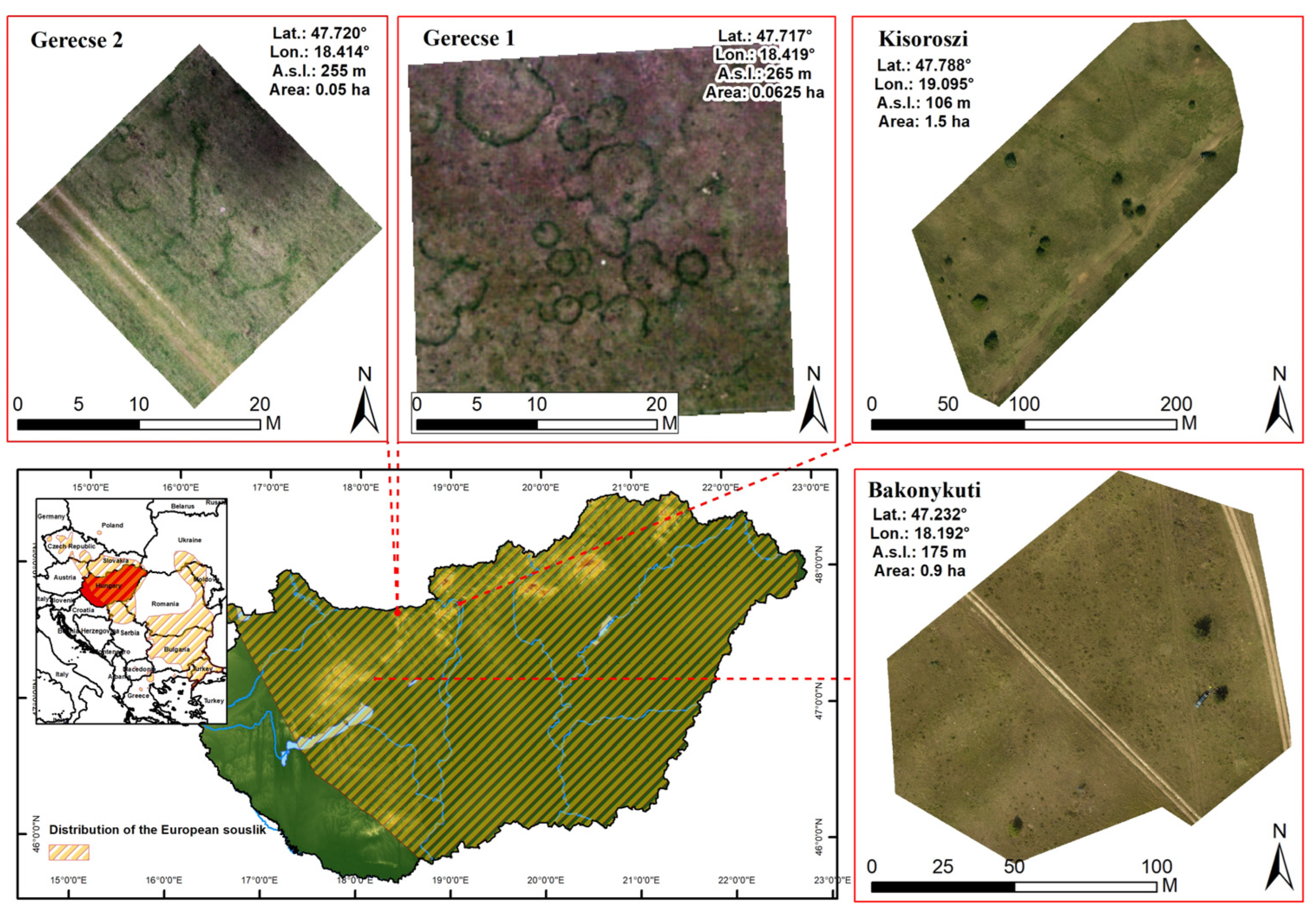
2.1. Field Survey

We collected images of four souslik colonies in the sampled areas between 1 and 31 July 2019 in Hungary with UAV imagery. Study sites were in coordinate system UTM/Zone 33 (Figure 1).

The colonies were found in different regions of Hungary and had short to medium-height grass [21]. Preliminary studies indicated that tall grass (mean > 18 ± 1.5 cm) disabled the application of UAV imagery and semi-automated detection due to the obscuration of BOs. Therefore, we excluded one site from the analysis in advance. We designated the study areas as Bakonykúti, Gerecse I, Gerecse II, and Kisoroszi.

All four colonies were located in the Pannonian grassland ecoregion. Xerophilous loess grassland of Salvio nemorosae-Festucetum rupicolae dominated three colonies (Bakonykúti, Gerecse I and Gerecse II; Ref. [60] and Festucetum vaginatae characterized the open sand grassland of the Kisoroszi colony [18]. Annual grass, perennial herbs, shrubs, and small trees dominated all grasslands. Each study site was under legal protection and located in a national park. This allowed little tourism at study sites, and they primarily served conservation aims. Grazing by sheep maintained short or medium-short vegetation all year around at all four sites which benefited sousliks’ survival and helped detect BOs in the field and on images.

We marked the exact locations of active animal BOs in the field with red–white–yellow flags (Figure S1). Then we took the first images of each area, removed the flags, and repeated the image recording process. This approach enabled us to find almost all BOs on each image visually and to use the flag-free images for further processing. The reports of the annual state monitoring and our visual observations of animals or their pellets at the BOs validated all four colonies as active souslik populations, and determined the core area of the colonies reliably.

We conducted the aerial surveys at all four test sites using a UAV with a visible range (RGB) camera onboard after we surveyed the area and marked each BO. After a few pilot surveys (with a 16 Mpx Ricoh GR II camera) on the Gerecse areas, we found a 24 Mpx Fuji X-T20 camera appropriate for the survey (main features: APS-C sensor; focal length of 14 mm; f/2.8 mm; automatic ISO speed; automated exposure time based on the sharpness, color saturation, and brightness of input images) (Table S1). We performed the aerial surveys in a fully automatic flight mode above the study area with image overlap of 80% and sidelap of 60% to ensure photogrammetric processing later. The focal length and resolution at an altitude of 25 m were found to be sufficient for recording BOs on a number of pixels. For later image orthorectification, we placed four or more ground control points at each site with a real-time kinematic correction GPS receiver unit (South Galaxy G1) with a maximum 1 cm error (horizontal and vertical accuracy). We used those ground control points to transform raw images into a Hungarian national coordinate system (EOV/HD72—EPSG:23700).

2.2. Statistical Analyses

We performed all statistics using TIBCO Statistica (2018; Version 13.5.0.17) and R (Version 4.0.1.3) [61,62,63]. More specifically, the algorithm used for calculating accuracy metrics was developed in R, but the confusion matrix and RF classification were calculated in Statistica. We also used R for analyzing spatial patterns, spectral transformations, and index generation using the Raster and RSToolbox packages. If we did not determine a level of significance in a specific analysis, then we generally used p < 0.05.

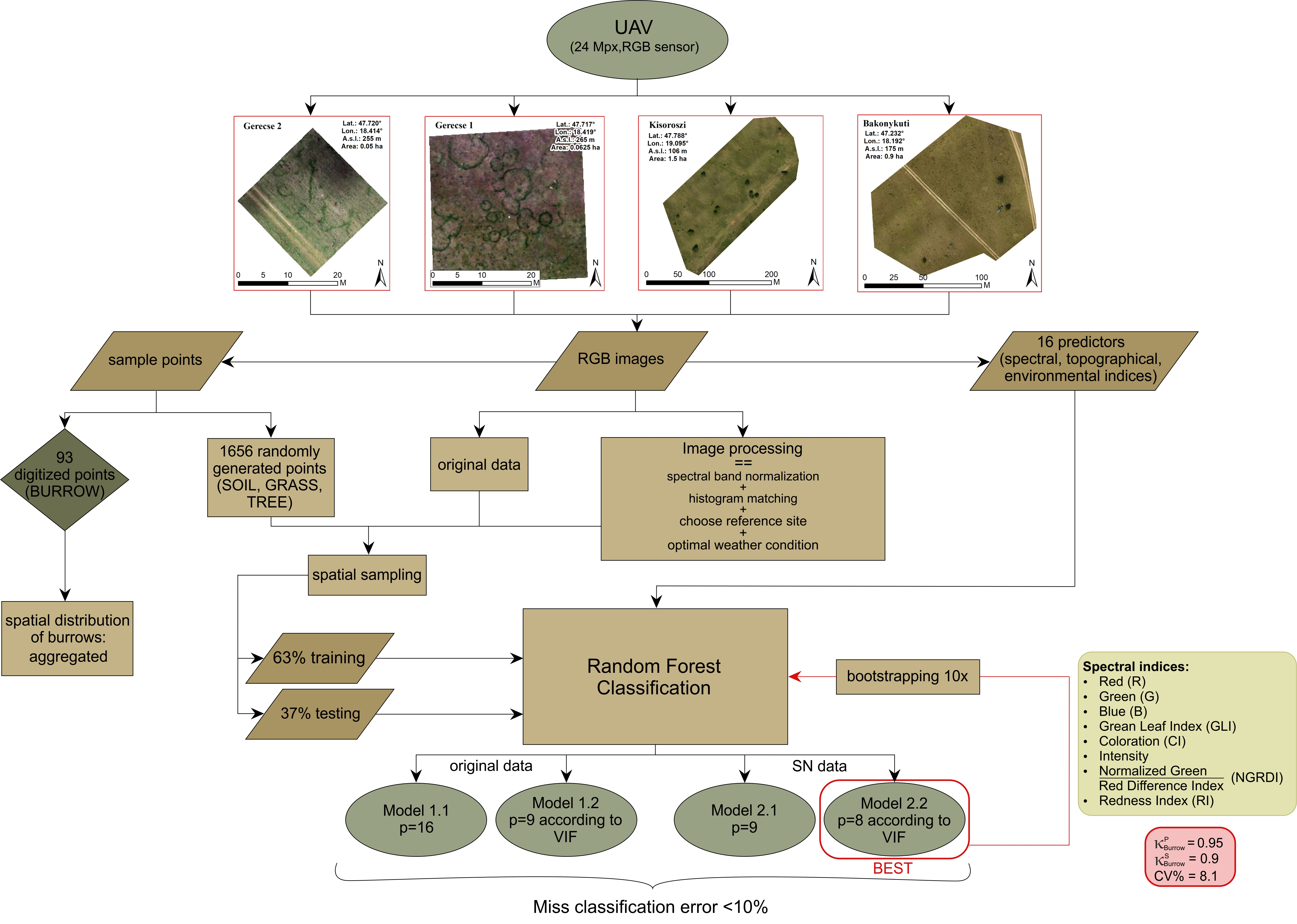
2.3. UAV Imagery and Spectral Data Pre-Processing

The image processing started with RGB unmanned aircraft system imagery in the field. A photogrammetric workflow including orthorectification followed UAV imagery, which resulted in an orthophoto mosaic to be processed by a supervised PBI [45,46,64]. The latter resulted in RGB derived spectral indices calculated from cloud-free and corrected RGB reflectance bands of any point (pixel) on the image. The raw images were processed in Agisoft Metashape Professional (Version 1.6.1) [65] to create RGB orthomosaics and digital elevation models (DEM) of the study sites. Thus, we ended up with four datasets, each transformed into the UTM/Zone33 coordinate system at 1 cm spatial resolution. At this scale, one average burrow opening (3–4 cm in diameter) covered ~7–12 pixels, which was enough to find a “pure” burrow pixel.

To increase orthomosaic similarity between images of the study sites for spectral sampling of field categories, consecutive processing steps were carried out on the mosaic images: histogram matching and spectral band normalization. First, we chose the orthomosaic of the Kisoroszi site as a reference histogram because atmospheric and flying conditions (at noon, without clouds) were optimal. Then we transformed all other histograms in comparison with that reference site. Secondly, we generated spectral indices based on the raw values of RGB bands. Then those raw values were normalized and centered. This image processing eventually resulted in predictors to be used in random forest (RF) classification (

Table 1. List and descriptions of input variables (predictors) for the four RF models (M1.1, 1.2, 2.1, 2.2).

Variable Acronym	Variable’s Long Name	Type	Reference or Description	Model
R	Red	Spectral	Red colour band	M1.1-2, M2.1-2
G	Green	Spectral	Green colour band	M1.1-2, M2.1-2
B	Blue	Spectral	Blue colour band	M1.1-2, M2.1-2
GLI	Green Leaf Index	Spectral	[66]	M1.1-2, M2.1-2
CI	Coloration Index	Spectral	[67]	M1.1-2, M2.1-2
Intnsty	Intensity	Spectral	[67]	M1.1-2, M2.1-2
NGRDI	Normalized Green/Red Difference Index	Spectral	[68]	M1.1-2, M2.1-2
RI	Redness Index	Spectral	[69]	M1.1-2, M2.1-2
SLP	Slope	Topographical	[70]	M1.1
ASP	Aspect	Topographical	[71]	M1.1
TPI	Topographioc Position Index	Topographical	[72]	M1.1
TRI	Topographic Ruggedness Index	Topographical	[73]	M1.1
Rghness	Roughness	Topographical	[73]	M1.1
DEM	Digital Elevation Model	Topographical	[74]	M1.1, M2.1
Grass height	Grass height	Topographical	Estimated height of surface point	M1.1
Site	Study site	Environmental	Study site	M1.1

).

We digitized the individually flagged BOs on orthomosaics in QGIS [75] by placing vector points on the central pixel. The burrow openings were always the darkest pixels on images. Therefore, those darkest pixels could always represent the BOs unambiguously. Burrows, trees, grass, and soil were the most characteristic and redundant field cover features of the sites. For better determination of category-specific spectral characteristics, we generated a different number of samples for the categories TREE, GRASS, and SOIL. The more difficult it was to distinguish a category from BURROW, the more samples we generated for that category to encompass its natural spectral variability. Since GRASS was the noisiest relative to BURROW, due to things such as shadows from grass tussocks near BOs, we generated a high number of samples representing grass. We found a total of 89 burrows in the four sites. In addition, we generated 108 TREE, 164 SOIL, and 1381 GRASS random points on all four sites.

2.4. Random Forest Classification of Pixels

The main purpose of RF classification was to correctly identify BOs on images (category BURROW). Following the recommendations of statistical textbooks [55,76,77], the numbers of decision trees (ntree) and randomly chosen input variables (mtry) were set to 500 and 4 or 3, respectively (mtry = p^1/2, where p is the total number of predictors; Breiman, 2001; Table 1). To decrease model complexity, we identified important predictors from the initial set of predictors (spectral, topographic, and environmental variables and indices) based on the variable importance scores (VIS). This approach clarified the simplest but still most robust model for the classification. We used a total of 16 predictors and raw images in the initial model, Model 1.1 (M1.1). Then, the number of predictors was reduced (p = 9), and a new RF model, Model 1.2 (M1.2), was built. The third (Model 2.1, M2.1) (p = 9) and fourth (Model 2.2, M2.2) models (p = 8) used spectrally normalized images. The predictor site represents the general characteristics of the habitat (Table 1). Since we wanted to see if histogram matching and spectral band normalization could improve model performance, we ran RF classification on both raw (M1.1 and 1.2) and spectrally normalized images (M2.1 and 2.2). Various metrics of overall and per-class accuracy of classification were used to determine how successfully each model identified BOs on images. During RF model building, 63% of the original dataset was used for training and 37% for testing to avoid overfitting [78].

2.5. Evaluation of RF Classification

The correctness of the classification procedure was measured by the number of correct or incorrect classifications of points. Actual values could be “true” or “false,” and predicted values could be “positive” or “negative,” The terms True Positive (TP), False Positive (FP), True Negative (TN), and False Negative (FN) covered all options regarding the classification results. The different numbers and ratios of those probabilities expressed by overall accuracy, Cohen’s kappa, precision and sensitivity, and F-score were used to evaluate the performances of the classification models, in other words, how accurately the models classified actual pixels into one of the four RF categories. The classification models’ overall performance levels were compared by overall accuracy (OA; (TP + TN)/total).

Cohen’s kappa (κ)

$$\mathsf{\kappa }=\frac{\mathrm{observed} \mathrm{accuracy}-\mathrm{chance} \mathrm{agreement}}{1-\mathrm{chance} \mathrm{agreement}}$$

Refs. [53,79] evaluated the agreement between predicted classification and actual values. It evaluated the correctness of the classification performed in comparison to randomly assigning values to one of the four categories. The κ can generally range from 0 to 1. A positive value would indicate that the classification is better than a random classification, whereas 0 would indicate that the classification does not perform better than a random classification process. According to our premise, we punished a misclassification of a souslik burrow (False Negative) and a misclassification of anything as a burrow (False Positive) equally, as we wanted to identify souslik Bos, and the correct or false classification of other objects in the environment (GRASS, TREE, SOIL) was left out of this evaluation. Per-class Cohen’s kappa (κ_BURROW) for producers’ (sensitivity, S, $\frac{\mathrm{TP}}{\left(\mathrm{TP}+\mathrm{FN}\right)}$) and users’ accuracies (precision, P, $\frac{\mathrm{TP}}{\mathrm{TP}+\mathrm{FP}}$), and F-score ( $\frac{2\times \mathrm{S}\times \mathrm{P}}{\mathrm{S}+\mathrm{P}}$ ), which punished extreme values and differences between these two values more than other means, characterized te BURROW-specific performance of the models and the relationship between the predicted and actual numbers of souslik BOs.

2.6. Model Stability

We evaluated the stability of the best model with 10-iteration bootstrapping. The number of decision trees (ntree) and number of input variables (mtry) were set to 500 and 3 respectively. With this iteration process, we could calculate and compare standard deviation (SD) and coefficient of variation (CV%) of κ between models (M2.2₁, M2.2₂, …, M2.2₁₀). One test of model stability involved testing if the variance of κ_BURROW for P and S (One sample test for variance) (1) was smaller than the average of the CV% of κ_BURROW for P and S of Models 1.1, 1.2, and 2.1, and (2) could remain ≤5% for either S or P. We defined CV% of a parameter in a population as the ratio of the standard deviation (SD) to the mean, and it was a dimensionless measure and considered a measure of stability of a population parameter. In our case, κ_BURROW for P and S could be those parameters whose low variance across the iteration could be used to evaluate the stability of the final RF model. Since the test of a single variance assumed a normal distribution of the population parameters, we tested normality with a modified Kolmogorov–Smirnov–Lilliefors test for small sample size.

2.7. Spatial Distribution of Burrows (Mounds or/and BOs)

We performed point pattern analysis to investigate the spatial distribution of burrows at the study sites and to explore the potential interaction between the burrows. This meant to justify the need for our method compared to the notion that animals occupy the space randomly or uniformly. We computed the $G\left(r\right)$ nearest neighbour distances distribution function and the $F\left(r\right)$ empty space function for all study sites, assuming the burrows constitute a point pattern $\mathrm{X}$ at a study site. This was to explore whether there was an interaction between the location of the burrows, and if there was, then what type of interaction it could be. The $G\left(r\right)$ function measured the distribution of the distances from an arbitrary burrow to its nearest neighbour (i.e., the burrow nearest to it), that is,

$$G\left(r\right)=\mathrm{P}\left\{d\left(u,\mathrm{X} \backslash \left\{u\right\}\right)\le r | u\in \mathrm{X}\right\}$$

where $u$ is an arbitrary burrow, and $d\left(u,\mathrm{X} \backslash \left\{u\right\}\right)$ is the shortest distance from $u$ to the point pattern $\mathrm{X}$, excluding $u$ itself. The $F\left(r\right)$ function measured the distribution of all distances from an arbitrary point of the plane to its nearest burrow, that is,

$$F\left(r\right)=P\left\{d\left(v,\mathrm{X}\right)\le r\right\}$$

where $v$ is an arbitrary point of the plane and $d\left(v,\mathrm{X}\right)$ is the distance from $v$ to the point pattern $\mathrm{X}$. At all study sites we compared the observed $G\left(r\right)$ and $F\left(r\right)$ functions to the Poisson point process (complete spatial randomness, CSR), which helped us decide the type of interaction that existed between the BOs. If the observed $G\left(r\right)$ ($F\left(r\right)$) function was below (above) CSR, then the distribution of BOs at the study site was rather regular. If the $G\left(r\right)$ ($F\left(r\right)$) was above (below) CSR, then the burrows showed a clustered pattern. To test whether this difference between the observed functions and CSR was significant, we simulated the upper and lower envelopes of CSR at each study site using the Monte Carlo approach.

3. Results

3.1. Evaluation of RF Classification

Overall accuracy of each model (from M1.1 to M2.2) (

Table 2. Overall accuracies and kappa statistics, per-class BURROW kappa for S (${\mathsf{\kappa }}_{BURROW}^s$ ) and P (${\mathsf{\kappa }}_{BURROW}^P$ ), and their parameter estimates for each RF model. Coefficient of variation (CV%), confidence interval (CI).

	Model 1.1	Model 1.2	Model 2.1	Model 2.2
Overall Accuracy	92.49	95.01	92.10	91.31
Standard Deviation	1.16	0.97	1.18	1.24
CV%	1.30	1.00	1.30	1.40
95% CI lower	90.12	93.00	89.68	88.79
95% CI upper	94.85	97.02	95.42	93.83
Cohen’s Kappa	0.76	0.84	0.76	0.74
Standard Deviation	0.04	0.03	0.04	0.04
CV%	4.6	3.6	4.6	5.0
95% CI lower	0.69	0.78	0.69	0.66
95% CI upper	0.83	0.90	0.83	0.81
${\mathbf{\kappa }}_{\mathit{BURROW}}^{\mathit{P}}$	0.90	1.00	1.00	0.95
Standard Deviation	0.07	0.00	0.00	0.05
CV%	7.40	0.00	0.00	4.90
${\mathbf{\kappa }}_{\mathit{BURROW}}^{\mathit{s}}$	0.75	0.59	0.91	0.90
Standard Deviation	0.09	0.10	0.06	0.07
CV%	11.70	16.80	6.70	8.10

) was above 90%, which meant less than 10% overall or misclassification error for each model.

Predictors R, G, B, GLI, CI, intensity, NGRDI, and RI were important for all four models (Table 1). Those eight spectral predictors remained relevant in M1.2, M2.1, and M2.2, while other environmental or topographic predictors were ignored based on VIS. The κ indicated the highest overall performance was for M1.2 (Table 2). The other models performed worse according to κ, though the difference between M1.2 (the highest score) and M2.2 (the lowest score) was small (0.84 vs. 0.74).

Per-class (BURROW) model performance (P_BURROW, S_BURROW, κ_BURROW) was the primary focus of our classification, as we wanted to train our models to automatically identify souslik burrows on images and achieve high and balanced precision and sensitivity. The confusion matrix (Table S2 for M2.2) could show all performance measurement values; however, here we focus only on those values that reflected per-class BURROW model performances. M2.1 had the highest (0.96) and M1.2 the lowest (0.75) F-scores. The other two models’ F-scores are in line with the distinction between the accuracy metrics based on raw or spectrally normalized data (F-score_M1.1 = 0.83; F-score_M2.2 = 0.91). Regarding the difference between P_BURROW and S_BURROW values, M2.2 had the lowest difference (0.08) while M1.2 had the greatest difference (0.4). Concerning κ_BURROW for P and S, Models 1.2 and 2.1 had the highest values, M2.2 trailed by 0.05, and M1.1 by an additional 0.05 (Table 2).

3.2. Model Stability

The standard deviation of κ was significantly less than the test variance, which was determined as the average SD of κ of models 1.1, 1.2, and 2.1 ($AV{G}_{SD}^{M1.1,1.2,2.1}$ = 0.034, n = 10, Chi-square of κ = 5.19 × 10⁻⁴, p = 1.36 × 10⁻¹⁸;

Table 3. How per-class (BURROW) Cohen’s kappa, standard deviation (SD), and coefficient of variation (CV%) for precision and sensitivity changed during the 10 iterations. For each iteration, different training (63%) and test (37%) subsets were selected randomly from the complete dataset.

	Iteration	Cohen’s Kappa for Precision	SD	CV%	Cohen’s Kappa for Sensitivity	SD	CV%
Per-class (BURROW)	1	0.96	0.04	4.30	0.85	0.07	8.00
	2	0.82	0.06	7.10	0.95	0.04	3.80
	3	0.79	0.06	7.90	0.97	0.03	2.90
	4	1.00	0.00	0.00	0.84	0.06	7.20
	5	0.94	0.04	4.70	0.91	0.05	5.60
	6	0.97	0.03	3.30	0.94	0.04	4.50
	7	0.96	0.04	3.70	0.87	0.06	7.00
	8	0.97	0.03	3.40	0.85	0.06	7.10
	9	0.85	0.06	7.30	0.82	0.07	7.90
	10	1.00	0.00	0.00	0.90	0.05	5.80

).

Levene’s test of the homogeneity of variances showed that the variances of CV% for κ_BURROW for P and S did not differ significantly (n = 10, F = 1.74, p = 0.20). Moreover, the average CV% of models 1.1, 1.2, and 2.1 for κ_BURROW for P and S were 2.47 (P) and 11.73 (S). The variance of CV% for κ_BURROW for P or S was significantly smaller than the hypothetical (test) variance of 5% (CV% = 5, n = 10, Chi-square of κ for p = 0.022, p = 1.23 × 10⁻¹²; Chi-square of κ for S = 0.0023, P = 1.17 × 10⁻¹⁷). Both the Kolmogorov–Smirnov–Lilliefors and Shapiro–Wilk tests of normality suggested that both S and P followed a normal distribution; therefore, the “one sample test for variance,” could be used and the normality assumption was not violated (P: Shapiro–Wilk statistic = 0.87, P = 0.086; KS–Lilliefors statistic = 0.23, P = 0.10; S: Shapiro–Wilk statistic = 0.93, P = 0.39; Lilliefors statistic = 0.16, P = 0.20).

3.3. Spatial Pattern of BOs

The point pattern analysis (G(r): the nearest neighbor metric, F(r): the so-called empty-space function metric) performed on the souslik BOs as proxies for the presence and locations of animals indicated clustered spatial patterns at (i) Bakonykúti and Kisoroszi: a statistically significant and strong spatial aggregation point pattern, (ii) Gerecse I: a statistically significant but weak spatial aggregation. A nearly random spatial pattern was present at Gerecse II (Figure S2). The results showed that the spatial distribution of the BOs tended to appear in groups rather than in regular or uniform patterns.

4. Discussion

Our results supported the aggregated distribution of souslik burrows. This highlights the need for the survey of BOs in the whole area of occupancy if spatial boundaries or density changes of colonies over large areas are to be detected. Souslik colonies can cover several hectares; consequently, the estimation of their abundance or area of occupancy by detecting and counting burrow openings would require a comprehensive survey of large areas. Our UAV-imagery-based method achieved adequate accuracy and reliability in detecting burrows semi-automatically. The final model (M2.2) was stable [39,80,81] and showed (1) balanced numbers of FN and FP detections, (2) high and balanced per-class (BURROW) accuracy metrics between training and testing subsets or P and S values, and (3) a user-friendly (less costly and easy to use) and straightforward counting method of BOs. Nevertheless, the number of burrow openings of a burrow system belonging to one individual requires a narrower estimation in the future by other proximal sensing techniques. On the other hand, automated detection and counting of BOs were addressed successfully by our method (Figure S3). This means that it is ready to be established in the management of endangered souslik populations or modified to the characteristics of other burrowing mammals’ burrows. Censusing of animal populations is a prerequisite for their adequate management [40,82], and BOs provide good proxies for population estimation.

Technical Issues

The use of a 24 Mpx RGB sensor and spectral normalization, including correction and standardization of illumination and color using a reference site, improved the accuracy of detection of burrows. The optimal weather conditions for imagery at one site could provide a good reference for correcting other images. Those conditions (less obscuration of BOs and strong natural light illumination) at the reference site could have provided less spectral noise or overlap which otherwise could have decreased the performance of RF classification [83]. That image processing substantiated RF classification of image pixels effectively into categories with high P and S (over 90% accuracy). RF classification on raw images resulted in a few FPs (high P, low overestimation), but S was low and much rarer than P. This meant a high number of FNs; consequently, we missed a number of burrows on those raw images. In a survey, that would have resulted in the underestimation of BOs, which would have indicated lower abundance or a smaller area of occupancy than the actual one. The imbalance between the numbers of FNs (high) and FPs (low) of the category BURROW was smoothed out (measured by κ_BURROW for P and S) by the application of spectral normalization, which was able to generate a smaller difference between FNs and FPs and still provide high TPs and TNs (Table 2). Although a small decrease in these accuracy measures was experienced after spectral normalization, κ_BURROW for S and P remained high (0.9) [84] and the FN × FP⁻¹ ratio was balanced. Balanced and still high S and P values were superior compared to higher and unbalanced S or p values, as either under- or overestimation would have been equally misleading [85]. Notwithstanding, those balanced values may not remain stable for other samples, so how stable this FN × FP⁻¹ ratio remains should be tested further in the future.

Results indicated the irrelevance of DEM or micro-relief (unexpected) and site (expected) as predictors in classifying and detecting BOs successfully (M1.2, 2.2). This could be explained by the homogeneity of sites and insignificant difference between the frequency of BOs on elevations and depressions. Grass height was found to be unimportant in the RF classification. Within the acceptable range of grass height (short and medium high), shadows generated by grass tussocks did not obscure the few-centimeter-high BOs. As European sousliks abandon habitats where grass becomes tall, the problem of grass tussock shadows that could be confused with the darkness of BOs in the RGB channels and frequencies (spectral mixing) is not a real problem of concern. Certainly, it would still be possible to decrease the number of FN detections in tall grass by adding further spectral channels to sense with the application of hyper/multispectral or thermal cameras. Nevertheless, natural monitoring in any country focuses on estimating the number of burrows in existing local populations and not on exploring new, probably isolated, and small colonies living in suboptimal, tall grass circumstances.

Literature suggests an aggravated pattern of sousliks and burrows is due to behavioral (nepotism) or habitat characteristics (elevations) [86,87]. Therefore, more mountainous souslik habitats with steep slopes, as in areas in the Mediterranean (e.g., Greece and Bulgaria) might show a different picture from the perspective of site homogeneity and spatial distribution of animals. Certain micro-elevations can help sousliks survive flooding or avoid predators [21,35], but its importance is probably habitat-specific and may change with the slope of an area.

Homogenous habitat and physiological characteristics through the distribution range of a species and model stability are prerequisites to good model transferability, though there has not been a standardized way to measure that [88]. Therefore, testing the final model’s stability was crucial for the method’s application. To improve stability and the potential of transferability, careful attention was paid to sampling, data quality, and model parsimony. For careful sampling, we took images of areas with souslik burrows after meticulously searching them for occupancy of BOs. Finding quasi- and verified burrows on sites increased the sample size. BOs appear almost identical (dark holes) and the inter-category spectral differences between BURROW, SOIL, GRASS, and TREE were expected to be much larger than the intra-category variation due to different plants, souslik burrows, and soil types (calcareous soils including sandy loess, loess, or chernozem) at different locations. Sampling at various locations with larger environmental dissimilarities improves model transferability [88,89]; however, the environmental similarity of souslik habitats in the Pannonian ecoregion did not support colonies sampled far away because it would not have meant a larger environmental difference. Consequently, the relative proximity of selected colonies (Figure 1) did not theoretically decrease model transferability. For increased data quality and a more universal model, the four datasets were merged, and 63% of data were randomly selected from the combined dataset to train RF classification. The approach of Jin et al. [90] contributed to building a more location-independent model. For a more parsimonious model, the simplest model with high and balanced accuracy was chosen as the best model (between S and P; small variation of Cohen’s kappa and its standard deviation; Table 2). All these considerations have helped and supported that the final model could be a good candidate for a universal model (reasonable, feasible, with good transferability potential) in spite of the small number of local populations in this study. Future research will encompass the study of transferability in different souslik populations, and we plan to expand the method into other ground dwelling species [88].

5. Conclusions

To summarize, we can clearly argue that the best model efficiency when detecting burrows accurately was high (~0.9) enough to be applied to counting burrows or delineating areas occupied by European sousliks. Our primary aim was to demonstrate that the semi-automated burrow detection and counting could provide a fair estimation of the number of burrows in a souslik colony (low quantity error). This approach is less concerned about how accurately burrows were localized. This means that if our future research aims at mapping or localizing burrows in space, then more classifiers, deep learning algorithms combined with more advanced imagery, will probably improve the local accuracy of burrow mapping. In other words, there is still room for improving the accuracy of burrow detection and counting by applying further and more advanced remote sensing techniques (multi- or hyperspectral or thermal cameras), approaches (segmentation and template matching), and classification methods (neural-network-based image classifiers) [91]. Those tools and methods are expected to better deal with the potential problem of shadows being confused with burrows. Then, spectral differences between natural shadows and dark burrow openings in the field may become more obvious and more easily distinguishable. With this, suboptimal weather conditions during field imagery may also become a less important factor to consider. Further research in that direction needs to compare the accuracy of different models. Then, a comparison of those different methods and measures of accuracy would also require more advanced accuracy measurements than kappa statistics [92,93].

However, this ready-to-use, non-invasive, simple approach reported in the manuscript can provide a useful tool for conservationists to count animal burrows used for population monitoring without much expertise in or resources for remote sensing. The application of this approach can be used to augment souslik or other burrowing mammal monitoring (e.g., mole rats and moles) using done by laborious manual counting of animal burrows.

References

1. Feldhamer, G.; Drickamer, L.; Vessey, S.; Merritt, J. Mammalogy: Adaptation, Diversity, Ecology; 3rd ed.; JHU Press: Baltimore, MD, USA, 2007. [Google Scholar]
2. Gomes Rodrigues, H.; Šumbera, R.; Hautier, L. Life in Burrows Channelled the Morphological Evolution of the Skull in Rodents: The Case of African Mole-Rats (Bathyergidae, Rodentia). J. Mamm. Evol. 2016, 23, 175–189. [Google Scholar] [CrossRef] [Green Version]
3. Meadows, P.S.; Meadows, A. The Environmental Impact of Burrowing Animals and Animal Burrows. In Proceedings of the Symposium, London, UK, 3–4 May 1990, 1st ed.; Published for the Zoological Society of London by Clarendon Press: London, UK, 1991; ISBN 0198546807. [Google Scholar]
4. Haussmann, N.S. Soil Movement by Burrowing Mammals: A Review Comparing Excavation Size and Rate to Body Mass of Excavators. Prog. Phys. Geogr. 2017, 41, 29–45. [Google Scholar] [CrossRef] [Green Version]
5. Hansell, M.H. The Ecological Impact of Animal Nests and Burrows. Funct. Ecol. 1993, 7, 5. [Google Scholar] [CrossRef]
6. Whitford, W.G.; Kay, F.R. Biopedturbation by Mammals in Deserts: A Review. J. Arid Environ. 1999, 41, 203–230. [Google Scholar] [CrossRef]
7. Sandifer, P.A.; Sutton-Grier, A.E.; Ward, B.P. Exploring Connections among Nature, Biodiversity, Ecosystem Services, and Human Health and Well-Being: Opportunities to Enhance Health and Biodiversity Conservation. Ecosyst. Serv. 2015, 12, 1–15. [Google Scholar] [CrossRef] [Green Version]
8. Brevik, E.C.; Slaughter, L.; Singh, B.R.; Steffan, J.J.; Collier, D.; Barnhart, P.; Pereira, P. Soil and Human Health: Current Status and Future Needs. Air Soil Water Res. 2020, 13, 1178622120934441. [Google Scholar] [CrossRef]
9. Davidson, A.D.; Lightfoot, D.C. Interactive Effects of Keystone Rodents on the Structure of Desert Grassland Arthropod Communities. Ecography 2007, 30, 515–525. [Google Scholar] [CrossRef]
10. Ewacha, M.V.A.; Kaapehi, C.; Waterman, J.M.; Roth, J.D. Cape Ground Squirrels as Ecosystem Engineers: Modifying Habitat for Plants, Small Mammals and Beetles in Namib Desert Grasslands. Afr. J. Ecol. 2016, 54, 68–75. [Google Scholar] [CrossRef]
11. Swaisgood, R.R.; Montagne, J.P.; Lenihan, C.M.; Wisinski, C.L.; Nordstrom, L.A.; Shier, D.M. Capturing Pests and Releasing Ecosystem Engineers: Translocation of Common but Diminished Species to Re-Establish Ecological Roles. Anim. Conserv. 2019, 22, 600–610. [Google Scholar] [CrossRef] [Green Version]
12. Lindtner, P.; Gömöryová, E.; Gömöry, D.; Stašiov, S.; Kubovčík, V. Development of Physico-Chemical and Biological Soil Properties on the European Ground Squirrel Mounds. Geoderma 2019, 339, 85–93. [Google Scholar] [CrossRef]
13. Butler, D.R. Zoogeomorphology: Animals as Geomorphic Agents; Cambridge University Press: Cambridge, UK, 1995. [Google Scholar] [CrossRef]
14. Johnson, D.L. Biomantle Evolution and the Redistribution of Earth Materials and Artifacts. Soil Sci. 1990, 149, 84–102. [Google Scholar] [CrossRef]
15. Hegyeli, Z. Spermophilus citellus. The IUCN Red List of Threatened Species 2020: E.T20472A91282380. Available online: https://dx.doi.org/10.2305/IUCN.UK.2020-2.RLTS.T20472A91282380.en (accessed on 4 March 2022).
16. Ramos-Lara, N.; Koprowski, J.L.; Kryštufek, B.; Hoffmann, I.E. Spermophilus Citellus (Rodentia: Sciuridae). Mamm. Species 2014, 913, 71–87. [Google Scholar] [CrossRef] [Green Version]
17. Erdos, L.; Tölgyesi, C.; Horzse, M.; Tolnay, D.; Hurton, Á.; Schulcz, N.; Körmöczi, L.; Lengyel, A.; Bátori, Z. Habitat Complexity of the Pannonian Forest-Steppe Zone and Its Nature Conservation Implications. Ecol. Complex. 2014, 17, 107–118. [Google Scholar] [CrossRef]
18. Győri-Koósz, B.; Faragó, S. Az Ürge (Spermophilus Citellus) Tápláléknövényei, Mint Potenciális Elterjedési Tényezők, Ökológiai Értékelésük Alapján. Magy. Apróvad Közlemények 2017, 13, 161–175. [Google Scholar] [CrossRef] [Green Version]
19. Šefferová, S.; Janák, M.; Vajda, Z. MANAGEMENT of Natura 2000 Habitats: Pannonic Sand Steppes; European Commission: Brussels, Belgium, 2008. [Google Scholar]
20. Ruzic, A. Citellus Citellus (Linaeus, 1766)—Der Oder Das Europäische Ziesel. In Handbuch der Säugetiere Europas, Bd. 1, Nagetiere I; Akad Verlagsgesellschaft: Wiesbaden, Germany, 1978; pp. 123–144. [Google Scholar]
21. Gedeon, C.I.; Boross, G.; Németh, A.; Altbäcker, V. Release Site Manipulation to Favour European Ground Squirrel Spermophilus Citellus Translocations: Translocation and Habitat Manipulation. Wildl. Biol. 2012, 18, 97–104. [Google Scholar] [CrossRef] [Green Version]
22. Mcdonald, B.L.L.; Stanley, T.R.; Otis, D.L.; Biggins, D.E.; Stevens, D.; Koprowski, J.L.; Ballard, W. Recommended Methods for Range-Wide Monitoring of Prairie Dogs in the United States; US Department of the Interior, US Geological Survey: Richmond, VA, USA, 2011; p. 36. [Google Scholar]
23. Willcox, D.; Nash, H.C.; Trageser, S.; Kim, H.J.; Hywood, L.; Connelly, E.; Ichu Ichu, G.; Kambale Nyumu, J.; Mousset Moumbolou, C.L.; Ingram, D.J.; et al. Evaluating Methods for Detecting and Monitoring Pangolin (Pholidata: Manidae) Populations. Glob. Ecol. Conserv. 2019, 17, e00539. [Google Scholar] [CrossRef]
24. Biggins, D.E.; Miller, B.J.; Hanebury, L.R.; Oakleaf, B.; Farmer, A.H.; Crete, R.; Dood, A. A Technique for Evaluating Black-Footed Ferret Habitat. In Management of Prairie Dog Complexes for the Reintroduction of the Black-Footed Ferret; US Fish and Wildlife Service Biological Report: Washington, DC, USA, 1993; Volume 13, pp. 73–88. [Google Scholar]
25. Harper, S.J.; Batzli, G.O. Effects of Predators on Structure of the Burrows of Voles. J. Mammal. 1996, 77, 1114–1121. [Google Scholar] [CrossRef] [Green Version]
26. Hubbs, A.H.; Karels, T.; Boonstra, R. Indices of Population Size for Burrowing Mammals. J. Wildl. Manage. 2000, 64, 296. [Google Scholar] [CrossRef] [Green Version]
27. Janák, M.; Marhoul, P.; Mateju, J. Action Plan for the Conservation of the European Ground Squirrel Spermophilus Citellus in the European Union List of Contributors; European Commission: Brussels, Belgium, 2013. [Google Scholar]
28. Csorba, G.; Pecsenye, K. Nemzeti Biodiverzitás-Monitorozó Rendszer X. Eml”osök És a Genetikai Sokféleség Monitorozása. Available online: https://scholar.google.com/scholar?hl=en&as_sdt=0%2C5&q=A+Nemzeti+Biodiverzitás-monitorozó+Rendszer+X.+Emlősök+és+a+genetikai+sokféleség+monitorozása&btnG= (accessed on 17 July 2021).
29. Váczi, O.; Varga, I.; Bakó, B. A Nemzeti Biodiverzitás-Monitorozó Rendszer Eredményei II—Gerinces Állatok; Körös-Maros Nemzeti Park Igazgatóság: Szarvas, Hungary, 2019. [Google Scholar]
30. Gedeon, C.I.; Hoffmann, I.E.; Váczi, O.; Knauer, F.; Ben Slimen, H.; Stefanović, M.; Lehoczky, É.; Laborczi, A.; Suchentrunk, F. The Role of Landscape History in Determining Allelic Richness of European Ground Squirrels (Spermophilus Citellus) in Central Europe. Hystrix 2017, 28, 240–246. [Google Scholar] [CrossRef]
31. Cepáková, E.; Hulová, S. Current Distribution of the European Souslik (Spermophilus Citellus) in the Czech Republic. Lynx 2002, 33, 89–103. [Google Scholar]
32. Stoeva, E.; Ivanov, I.; Stoev, I.; Yankov, L.; Mechev, A.; Koshev, Y. Successful Reinforcement of the European Souslik by Green Balkans NGO in “Sinite Kamani” Nature Park. In Annuaire de l’Université de Sofia “St. Kliment Ohridski” Faculte de Biologie; University Press: Sofia, Bulgaria, 2016; pp. 153–165. [Google Scholar]
33. Hoogland, J. (Ed.) Conservation of the Black-Tailed Prairie Dog: Saving North America’s Western Grasslands; Island Press: Chicago, IL, USA, 2013; Volume 88, ISBN 1559634979. [Google Scholar]
34. Hut, R.A.; Scharff, A. Endoscopie Observations on Tunnel Blocking Behaviour in the European Ground Squirrel (Spermophilus Citellus). Z. Fur Saugetierkd. 1998, 63, 377–380. [Google Scholar]
35. Katona, K.; Váczi, O.; Altbäcker, V. Topographic Distribution and Daily Activity of the European Ground Squirrel Population in Bugacpuszta, Hungary. Acta Theriol. 2002, 47, 45–54. [Google Scholar] [CrossRef]
36. Johson, D.L.; Burnham, J.L.H. (Eds.) Introduction: Overview of concepts, definitions, and principles of soil mound studies. In Mima Mounds: The Case for Polygenesis and Bioturbation: Geological Society of America Special Paper; 2012; Volume 490, pp. 1–99. [Google Scholar] [CrossRef]
37. Šumbera, R.; Mazoch, V.; Patzenhauerová, H.; Lövy, M.; Šklíba, J.; Bryja, J.; Burda, H. Burrow Architecture, Family Composition and Habitat Characteristics of the Largest Social African Mole-Rat: The Giant Mole-Rat Constructs Really Giant Burrow Systems. Acta Theriol. 2012, 57, 121–130. [Google Scholar] [CrossRef]
38. Velasco, M. A Quickbird’s Eye View on Marmots; International Institute for Geo-Information Science and Earth Observation: Enschede, The Netherlands, 2009. [Google Scholar]
39. Pettorelli, N.; Laurance, W.F.; O’Brien, T.G.; Wegmann, M.; Nagendra, H.; Turner, W. Satellite Remote Sensing for Applied Ecologists: Opportunities and Challenges. J. Appl. Ecol. 2014, 51, 839–848. [Google Scholar] [CrossRef]
40. Wang, X.; Zhang, F.; Kung, H.; Johnson, V.C. New Methods for Improving the Remote Sensing Estimation of Soil Organic Matter Content (SOMC) in the Ebinur Lake Wetland National Nature Reserve (ELWNNR) in Northwest China. Remote Sens. Environ. 2018, 218, 104–118. [Google Scholar] [CrossRef]
41. Swinbourne, M.J.; Taggart, D.A.; Swinbourne, A.M.; Lewis, M.; Ostendorf, B. Using Satellite Imagery to Assess the Distribution and Abundance of Southern Hairy-Nosed Wombats (Lasiorhinus Latifrons). Remote Sens. Environ. 2018, 211, 196–203. [Google Scholar] [CrossRef]
42. Wilschut, L.I.; Addink, E.A.; Heesterbeek, J.A.P.; Dubyanskiy, V.M.; Davis, S.A.; Laudisoit, A.; Begon, M.; Burdelov, L.A.; Atshabar, B.B.; de Jong, S.M. Mapping the Distribution of the Main Host for Plague in a Complex Landscape in Kazakhstan: An Object-Based Approach Using SPOT-5 XS, Landsat 7 ETM+, SRTM and Multiple Random Forests. Int. J. Appl. Earth Obs. Geoinf. 2013, 23, 81–94. [Google Scholar] [CrossRef] [Green Version]
43. Wilschut, L.I.; Heesterbeek, J.A.P.; Begon, M.; de Jong, S.M.; Ageyev, V.; Laudisoit, A.; Addink, E.A. Detecting Plague-Host Abundance from Space: Using a Spectral Vegetation Index to Identify Occupancy of Great Gerbil Burrows. Int. J. Appl. Earth Obs. Geoinf. 2018, 64, 249–255. [Google Scholar] [CrossRef]
44. Boyaci, D.; Erdoğan, M.; Yildiz, F. Pixel-versus Object-Based Classification of Forest and Agricultural Areas from Multiresolution Satellite Images. Turk. J. Electr. Eng. Comput. Sci. 2017, 25, 365–375. [Google Scholar] [CrossRef]
45. Vlachopoulos, O.; Leblon, B.; Wang, J.; Haddadi, A.; LaRocque, A.; Patterson, G. Delineation of Crop Field Areas and Boundaries from UAS Imagery Using PBIA and GEOBIA with Random Forest Classification. Remote Sens. 2020, 12, 2640. [Google Scholar] [CrossRef]
46. Vlachopoulos, O.; Leblon, B.; Wang, J.; Haddadi, A.; LaRocque, A.; Patterson, G. Delineation of Bare Soil Field Areas from Unmanned Aircraft System Imagery with the Mean Shift Unsupervised Clustering and the Random Forest Supervised Classification. Can. J. Remote Sens. 2020, 46, 489–500. [Google Scholar] [CrossRef]
47. Berhane, T.M.; Lane, C.R.; Wu, Q.; Anenkhonov, O.A.; Chepinoga, V.V.; Autrey, B.C.; Liu, H. Comparing Pixel- and Object-Based Approaches in Effectively Classifying Wetland-Dominated Landscapes. Remote Sens. 2018, 10, 46. [Google Scholar] [CrossRef] [PubMed] [Green Version]
48. Qu, L.; Chen, Z.; Li, M.; Zhi, J.; Wang, H. Accuracy Improvements to Pixel-Based and Object-Based LULC Classification with Auxiliary Datasets from Google Earth Engine. Remote Sens. 2021, 13, 453. [Google Scholar] [CrossRef]
49. Duro, D.C.; Franklin, S.E.; Dubé, M.G. A Comparison of Pixel-Based and Object-Based Image Analysis with Selected Machine Learning Algorithms for the Classification of Agricultural Landscapes Using SPOT-5 HRG Imagery. Remote Sens. Environ. 2012, 118, 259–272. [Google Scholar] [CrossRef]
50. Rokach, L.; Maimon, O. Ensemble Methods for Classifiers. In Data Mining and Knowledge Discovery Handbook; Springer-Verlag: Boston, MA, USA, 2006; pp. 957–980. [Google Scholar]
51. Berhane, T.M.; Lane, C.R.; Wu, Q.; Autrey, B.C.; Anenkhonov, O.A.; Chepinoga, V.V.; Liu, H. Decision-Tree, Rule-Based, and Random Forest Classification of High-Resolution Multispectral Imagery for Wetland Mapping and Inventory. Remote Sens. 2018, 10, 580. [Google Scholar] [CrossRef] [PubMed] [Green Version]
52. Dormann, C.F.; Elith, J.; Bacher, S.; Buchmann, C.; Carl, G.; Carré, G.; Marquéz, J.R.G.; Gruber, B.; Lafourcade, B.; Leitão, P.J.; et al. Collinearity: A Review of Methods to Deal with It and a Simulation Study Evaluating Their Performance. Ecography 2013, 36, 27–46. [Google Scholar] [CrossRef]
53. Lillesand, T.; Kiefer, W.R.; Chipman, J. Remote Sensing and Image Interpretation, 7th ed.; John Wiley & Sons: Hoboken, NJ, USA, 2015; ISBN 0471026093. [Google Scholar]
54. Janowski, L.; Tylmann, K.; Trzcinska, K.; Rudowski, S.; Tegowski, J. Exploration of Glacial Landforms by Object-Based Image Analysis and Spectral Parameters of Digital Elevation Model. IEEE Trans. Geosci. Remote Sens. 2022, 60, 1–17. [Google Scholar] [CrossRef]
55. Breiman, L. Random Forests. Mach. Learn. 2001, 45, 5–32. [Google Scholar] [CrossRef] [Green Version]
56. Biau, G.; Scornet, E. A Random Forest Guided Tour. Test 2016, 25, 197–227. [Google Scholar] [CrossRef] [Green Version]
57. Belgiu, M.; Drăgu, L. Random Forest in Remote Sensing: A Review of Applications and Future Directions. ISPRS J. Photogramm. Remote Sens. 2016, 114, 24–31. [Google Scholar] [CrossRef]
58. Smalheiser, N.R. Data Literacy: How to Make Your Experiments Robust and Reproducible, 1st ed.; Elsevier, Academic Press: London, UK, 2017; ISBN 9780128113066. [Google Scholar]
59. Delincé, J. Handbook on Remote Sensing for Agricultural Statistics. In Handbook on Remote Sensing for Agricultural StatisticsAgricultural Statistics; Delincé, J., Ed.; GSARS Handbook: Rome, Italy, 2017. [Google Scholar]
60. Zolyomi, B.; Fekete, G. The Pannonian Loess Steppe: Differentiation in Space and Time. Abstr. Bot. 1994, 18, 29–41. [Google Scholar]
61. Team, R.C. R: A Language and Environment for Statistical Computing; R Foundation for Statistical Computing: Vienna, Austria, 2020. [Google Scholar]
62. TIBCO Software Inc. Statistica (Data Analysis Software System), Version 13. 2018. Available online: http://statistica.io (accessed on 4 March 2022).
63. Bivand, R.; Gebhardt, A. Implementing Functions for Spatial Statistical Analysis Using the R Language. J. Geogr. Syst. 2000, 2, 307–317. [Google Scholar] [CrossRef]
64. Sibaruddin, H.I.; Shafri, H.Z.M.; Pradhan, B.; Haron, N.A. Comparison of Pixel-Based and Object-Based Image Classification Techniques in Extracting Information from UAV Imagery Data. IOP Conf. Ser. Earth Environ. Sci. 2018, 169, 12098. [Google Scholar] [CrossRef]
65. Agisoft, L. AgiSoft PhotoScan Professional (Version 1.2.6). 2016. Available online: http://www.agisoft.com/downloads/installer/ (accessed on 4 March 2022).
66. Louhaichi, M.; Borman, M.M.; Johnson, D.E. Spatially located platform and aerial photography for documentation of grazing impacts on wheat. Geocarto Int. 2001, 16, 65–70. [Google Scholar] [CrossRef]
67. Escadafal, R. Soil Spectral Properties and Their Relationships with Environmental Parameters—Examples from Arid Regions; Springer: Berlin/Heidelberg, Germany, 1994; pp. 71–87. [Google Scholar]
68. Zarco-Tejada, P.J.; Miller, J.R.; Mohammed, G.H.; Noland, T.L.; Sampson, P.H. Estimation of chlorophyll fluorescence under natural illumination from hyperspectral data. Int. J. Appl. Earth Obs. Geoinf. 2002, 2001, 321–327. [Google Scholar] [CrossRef] [Green Version]
69. Bannari, A.; Morin, D.; Bonn, F.; Huete, A.R. A review of vegetation indices. Remote Sens. Rev. 1995, 13, 95–120. [Google Scholar] [CrossRef]
70. Travis, M.R.; Iverson, W.D.; Elsner, G.H.; Johnson, C.G. VIEWIT: Computation of Seen Areas, Slope and Aspect for Land-Use Planning; USDA Forest Service: Berkeley, CA, USA, 1975; Volume 11. [Google Scholar]
71. Zevenbergen, L.W.; Thorne, C.R. Quantitative analysis of land surface topography. Earth Surf. Process. Landforms 1987, 12, 47–56. [Google Scholar] [CrossRef]
72. Guisan, A.; Weiss, S.B.; Weiss, A.D. GLM versus CCA spatial modeling of plant species distribution. Plant Ecol. 1999, 143, 107–122. [Google Scholar] [CrossRef]
73. Riley, S.J.; DeGloria, S.D.; Elliot, R. A Terrain Ruggedness Index that Qauntifies Topographic Heterogeneity. Intermt. J. Sci. 1999, 5, 23–27. [Google Scholar]
74. Hengl, T.; Reuter, H.I. (Eds.) Geomorphometry: Concepts, Software, Applications; 1st ed.; Developments in Soil Science, Elsevier: Amsterdam, The Netherlands, 2009; Volume 33. [Google Scholar]
75. QGIS Development, T. QGIS Geographic Information System: Open Source Geospatial Foundation Project; 2021. QGIS Association. Available online: http://qgis.osgeo.org (accessed on 4 March 2022).
76. Hastie, T.; Tibshirani, R.; Friedman, J. The Elements of Statistical Learning, 2nd ed.; Springer: New York, NY, USA, 2017; Volume 27, ISBN 978-0-387-84857-0. [Google Scholar]
77. Breiman, L.; Friedman, J.H.; Olshen, R.A.; Stone, C.J. Classification and Regression Trees, 1st ed.; Routledge: Boca Raton, FL, USA, 2017; ISBN 9781351460491. [Google Scholar]
78. Xu, Y.; Goodacre, R. On Splitting Training and Validation Set: A Comparative Study of Cross-Validation, Bootstrap and Systematic Sampling for Estimating the Generalization Performance of Supervised Learning. J. Anal. Test. 2018, 2, 249–262. [Google Scholar] [CrossRef] [Green Version]
79. Cohen, J. Weighted Kappa: Nominal Scale Agreement Provision for Scaled Disagreement or Partial Credit. Psychol. Bull. 1968, 70, 213–220. [Google Scholar] [CrossRef] [PubMed]
80. Stokes, E.; Johnson, A.; Rao, M. Monitoring Wildlife Populations for Management. Available online: https://www.researchgate.net/profile/Arlyne-Johnson/publication/257363333_Module_7_Monitoring_Wildlife_Populations_for_Management_Background_Presentation_and_Exercises/links/00463525085e5ab4ca000000/Module-7-Monitoring-Wildlife-Populations-for-Management- (accessed on 17 June 2021).
81. Stephenson, P.J. Integrating Remote Sensing into Wildlife Monitoring for Conservation. Environ. Conserv. 2019, 46, 181–183. [Google Scholar] [CrossRef]
82. Plumptre, A.J. Monitoring Mammal Populations with Line Transect Techniques in African Forests. J. Appl. Ecol. 2000, 37, 356–368. [Google Scholar] [CrossRef]
83. Agjee, N.H.; Mutanga, O.; Peerbhay, K.; Ismail, R. The Impact of Simulated Spectral Noise on Random Forest and Oblique Random Forest Classification Performance. J. Spectrosc. 2018, 2018, 1–7. [Google Scholar] [CrossRef] [Green Version]
84. Congalton, R.G. Accuracy Assessment and Validation of Remotely Sensed and Other Spatial Information. Int. J. Wildl. Fire 2001, 10, 321–328. [Google Scholar] [CrossRef] [Green Version]
85. Assal, T.J.; Lockwood, J.A. Utilizing Remote Sensing and GIS to Detect Prairie Dog Colonies. Rangel. Ecol. Manag. 2007, 60, 45–53. [Google Scholar] [CrossRef]
86. Sherman, P.W. Kinship, Demography, and Belding’s Ground Squirrel Nepotism. Behav. Ecol. Sociobiol. 1981, 8, 251–259. [Google Scholar] [CrossRef]
87. Weddell, B.J. Dispersion of Columbian Ground Squirrels (Spermophilus Columbianus) in Meadow Steppe and Coniferous Forest. J. Mammal. 1989, 70, 842–845. [Google Scholar] [CrossRef]
88. Sequeira, A.M.M.; Bouchet, P.J.; Yates, K.L.; Mengersen, K.; Caley, M.J. Transferring Biodiversity Models for Conservation: Opportunities and Challenges. Methods Ecol. Evol. 2018, 9, 1250–1264. [Google Scholar] [CrossRef] [Green Version]
89. Wenger, S.J.; Olden, J.D. Assessing Transferability of Ecological Models: An Underappreciated Aspect of Statistical Validation. Methods Ecol. Evol. 2012, 3, 260–267. [Google Scholar] [CrossRef]
90. Jin, S.; Su, Y.; Gao, S.; Hu, T.; Liu, J.; Guo, Q. The Transferability of Random Forest in Canopy Height Estimation from Multi-Source Remote Sensing Data. Remote Sens. 2018, 10, 1183. [Google Scholar] [CrossRef] [Green Version]
91. Wang, M.; Cui, Q.; Sun, Y.; Wang, Q. Photovoltaic Panel Extraction from Very High-Resolution Aerial Imagery Using Region–Line Primitive Association Analysis and Template Matching. ISPRS J. Photogramm. Remote Sens. 2018, 141, 100–111. [Google Scholar] [CrossRef]
92. Pontius, R.G.; Millones, M. Death to Kappa: Birth of Quantity Disagreement and Allocation Disagreement for Accuracy Assessment. Int. J. Remote Sens. 2011, 32, 4407–4429. [Google Scholar] [CrossRef]
93. Wu, S.S.; Qiu, X.; Usery, E.L.; Wang, L. Using Geometrical, Textural, and Contextual Information of Land Parcels for Classification of Detailed Urban Land Use. Ann. Assoc. Am. Geogr. 2009, 99, 76–98. [Google Scholar] [CrossRef]
Figure 1. Location of studied souslik colonies in Hungary, and area and spatial position of images used for image processing.
Remotesensing 14 02025 g001