Article

The Potential of Sentinel-1A Data for Identification of Debris-Covered Alpine Glacier Based on Machine Learning Approach

1
Nanjing Institute of Environmental Sciences, Ministry of Ecology and Environment, Nanjing 210042, China
2
School of Geography and Ocean Science, Nanjing University, Nanjing 210023, China
3
Department of Geophysical Engineering, Montana Technological University, Butte, MT 59701, USA
4
Institute of Tibetan Plateau Atmospheric and Environmental Sciences, Tibet Meteorological Bureau, Lhasa 850000, China
*
Author to whom correspondence should be addressed.
Remote Sens. 2022, 14(9), 1980; https://doi.org/10.3390/rs14091980
Submission received: 2 February 2022 / Revised: 3 April 2022 / Accepted: 12 April 2022 / Published: 20 April 2022
(This article belongs to the Section Remote Sensing Image Processing)

Abstract

:
Microwave remote sensing is one of the main approaches to glacier monitoring. This paper provides a comparative analysis of how different types of radar information differ in identifying debris-covered alpine glaciers using machine learning algorithms. Based on Sentinel-1A data, three data suites were designed: A backscattering coefficient (BC)-based data suite, a polarization decomposition parameter (PDP)-based data suite, and an interference coherence coefficient (ICC)-based data suite. Four glaciers with very different orientations in different climatic zones of the Tibetan Plateau were selected and classified using an integrated machine learning classification approach. The results showed that: (1) The boosted trees and subspace k-nearest neighbor algorithms were optimal and robust; and (2) the PDP suite (63.41–99.57%) and BC suite (55.85–99.94%) both had good recognition accuracy for all glaciers; notably, the PDP suite exhibited better rock and debris recognition accuracy. We also analyzed the influence of the distribution of glacier surface aspect on the classification accuracy and found that the more asymmetric it was about the sensor orbital plane, the more difficult it was for the BC and PDP suites to recognize the glacier, and a large slope could further reduce the accuracy. Our results suggested that during the inventory or classification of large-scale debris-covered alpine glaciers, priority should be given to polarization decomposition features and elevation information, and it is best to divide the glaciers into multiple subregions based on the spatial relationship between glacier surface aspect and radar beams.

1. Introduction

Glaciers are one of the most important water resources in the world. Most of them are concentrated in the high-altitude regions of the Earth’s mid- and low-latitudes and are usually important sources of fresh water and the birthplace of many glacier-driven rivers [1,2,3]. Glaciers are also an indicator of climate change and have positive feedback on climate [4,5]. In areas such as the Qinghai–Tibet Plateau (TP), the highest and largest plateau in the world [6], where glaciers have undergone dramatic area and volume retreat, these changes will affect the local climate and the meridional circulation of the atmosphere on a global scale owing to the large glacial area and high altitude [7,8]. The boundary of a glacier is the most direct parameter for monitoring its areal change. Remote sensing techniques are important and cost-effective tools for monitoring alpine glaciers [9,10,11]. However, many debris-covered glaciers are difficult to distinguish automatically from the surrounding rocky mountainous areas because of similar spectral characteristics, and remote sensing techniques require manual modification to improve identification accuracy [12]. Unlike optical remote sensing, radar can penetrate clouds and is independent of weather conditions; the penetration of radar also provides more information below the ground surface, which facilitates the identification of debris-covered glaciers [13,14]. Thus, synthetic aperture radar (SAR) is widely used for glacier monitoring, including its backscattering coefficient, coherence coefficient, and polarization decomposition features [15,16,17], which can identify debris-covered glaciers under various supervised and unsupervised classification algorithms. However, there are few comparisons of its effectiveness in a debris-covered alpine glacier inventory, so we aim to fill this gap in research.
During the radar remote sensing process, the incident and backscattered waves are mathematically represented by a scattering matrix, also known as the Sinclair matrix, where each element is a complex number representing the amplitude and phase angle [18]. The scattering matrix contains important attribute information about a target. According to the radar cross-section, the backscattered energy from each pixel of a radar image is obtained by averaging the power (intensity information) of a scattering matrix. The radar backscattering coefficient is generally expressed by the absolute value of the scattered radar power after calibration [18] and is the earliest and most used radar information. The dielectric constant, liquid water content, thickness and surface roughness of ice and snow, as well as the land surface types, will affect the backscattering properties of the targets and provide a theoretical basis for the classification of glacier zones [18,19,20,21,22].
The complex information about the physical and chemical properties of scatters within a pixel received by a radar antenna can be further deciphered by different scattering mechanisms, which usually have their own physical explanation [23]. The polarization mode of the backscattered wave is generally different from that of the incident wave because of depolarization and polarization spiral. This difference is described by both a covariance matrix and a coherency matrix that are converted from a scattering matrix [24]. The polarization decomposition converts the covariance and coherence matrices into a combination of different scattering matrices [22,25], allowing target classification, i.e., identification of a glacier based on polarization decomposition features [26]. This feature has also been often used in distinguishing dry and wet snow [27] and in identifying snow lines [21].
The phase difference between two single-look complex (SLC) radar images over the same area is the basis for radar interferometry. Once a ground pixel changes its position in the slant direction, the phase difference of that pixel is no longer zero [19,28]. In contrast to the backscattering coefficient and polarization decomposition characteristics, the coherence coefficient is a parameter that indicates the degree of similarity between an interference pair [29], with 0 to 1 representing complete decoherence to complete coherence. In general, the coherence coefficient is an effective parameter for monitoring surface deformation and classifying land surfaces [30,31,32,33,34]. In glacier identification, under the premise that the temporal and spatial baselines are controlled within an effective range, glacier motion induces low coherence but not complete decoherence; thus, the glacier can be distinguished from surrounding temporally stable objects regardless of land surface types [29,30]. However, the effectiveness of this method is limited when the deformation is caused by various factors [35] or the glacier moves too fast during the interference period. In addition, the wavelength also affects the interferometry effect: The longer the wavelength, the better the interference coherence [36].
The method for extracting glaciers from radar images has been improved with the enrichment of radar information types. Previous studies on glacier identification and classification have shown that the most used method for extracting glacier boundaries [37,38,39,40,41] is threshold segmentation of certain physicochemical parameters, texture information, or seasonal variations of radar parameter values associated with glaciers [37,42,43]. This method is simple and easy to implement, but the effectiveness of classification decreases when multiple factors constrain the threshold. With the development of artificial intelligence (AI), machine learning provided a computer system with the ability to access data, look for patterns in the data, make sound decisions with (supervised) or without (unsupervised) human intervention or assistance, and adjust actions accordingly. Machine learning has therefore attracted much attention in the identification and segmentation of targets in the cryosphere. Huang et al. [17] and Yao et al. [26] effectively classified a debris-covered glacier area by using the support vector machine (SVM) algorithm based on the difference in scattering mechanisms extracted by multi-polarization decomposition. Tsai et al. [44] used the simple tuning random-forest-based land-cover type-dependent classification strategy based on backscatter coefficients, polarization decomposition parameters, interferometric coherence coefficients, and four terrain features to calculate dry and wet snow in global mountainous regions. In the field of machine learning, in addition to the direct extraction of targets using hand-crafted features, there are also some algorithms that use high-level representations obtained through learning, which are far superior to the traditional technique based on hand-crafted features [45]. Robson et al. [46] successfully mapped 108 of 120 rock glaciers with the highest accuracy of 75.4% based on Sentinel-1 and -2 data using convolutional neural network (CNN) and object-based image analysis (OBIA). Cai et al. [45] used ResNet and improved atrous spatial pyramid pooling (ASPP) modules to extract multiscale features and used the decoder module to fuse high-level semantic features and low-level features to classify ice radar images at the pixel level accurately. Fabijańska et al. [47] developed a glacial varve detector based on CNN to delineate annual layers automatically. These deep learning algorithms learn more high-level features based on the labeled samples by fitting multiple convolutional layers, which facilitates target detection and image segmentation. However, an efficient deep learning network requires hundreds of input data layers, which means that success depends heavily on the quality and quantity of the training data. When the feature dimension exceeds a certain value, the performance of the classifier gradually deteriorates [48].
Sentinel-1 is the first of five satellite missions in the Copernicus program developed by the European Space Agency (ESA). It consists of two satellites, Sentinel-1A and Sentinel-1B, that share the same orbital plane and operate day and night to collect C-band SAR imagery, regardless of weather conditions. The repetition cycles are 6–12 days. The Sentinel-1A and B data are the most up-to-date publicly available SAR data; they have dual-polarization [49] and are widely used in cryospheric research, from monitoring ice sheets [50,51] and ice shelves [52,53] to sea ice melt [54,55] in polar regions. Lippl et al. [29] found Sentinel-1A had the lowest error rate in identifying glaciers among the interference coherence coefficients of the X, C, and L bands. However, few studies have used Sentinel-1A data for alpine glaciers, especially for debris-covered glaciers.
To investigate the effectiveness of different types of SAR information in identifying debris-covered alpine glaciers using Sentinel-1A data based on machine learning algorithms, we developed three types of data suites (suites of data sets) based on three primary SAR parameters: Backscattering coefficient (BC), polarization decomposition parameters (PDP), and interference coherence coefficient (ICC). Then we investigated the following questions: (1) Which machine learning algorithms are highly accurate and stable? (2) What type of data suite and which layers in each data suite are most effective in identifying debris-covered alpine glaciers? (3) How does the topography of glaciers affect the accuracy of glacier detection? This paper has the following structure: Section 2 describes the research sites and data sources we used; Section 3 describes all methods and procedures performed on Sentinel-1A SLC data. Section 4 shows the spatial distribution of the four glacier surface aspects, a comparative analysis of machine learning classification algorithms, and the best classification results using different data suites. Section 5 discusses the importance of layers within each data suite on classification accuracy, the influence of data suite type, and glacier aspect on glacier classification accuracy. Conclusions are drawn in Section 6.

2. Research Sites and Data

2.1. Research Sites

In the northwest of the TP, there are many continental glaciers formed by the alpine climate controlled by the westerlies. Because of the input of water vapor, glaciers in this area have remained stable in recent years, and some glaciers have even shown small progress [56]. In the central Himalayas, continental glaciers have been affected by the Indian monsoon, and glaciers in this region have retreated significantly in length and area in recent years [56]. In the southeast TP, the moisture from the Indian monsoon and the East Asian monsoon moves along the mountains and deep into the land, bringing warm precipitation and forming unique marine glaciers [57]. With the continuous retreat of glaciers under the influence of global warming, a sufficient supply of water vapor promotes the rapid movement of glaciers, causing many of them to become covered by debris. Therefore, we selected four glaciers with different main trunks in these three typical climatic zones as study sites (Figure 1). All are composite glaciers: There is a semicircular accumulation area at the source of the glacier with several tributary glaciers that converge in the middle and develop into an ice tongue at the end of the glacier in an almost constant direction.
Figure 1 shows the base map of the TP with three insets showing the four glaciers selected as study sites based on the main aspect of glacier surfaces. Four glaciers are shown as false-color images (RGB = band 3, band 5, and band 7, respectively) based on Landsat 8 Operational Land Imager (OLI) data. Tongue areas of all four glaciers are covered with rock debris, making them indistinguishable from the rocks on either side in the Landsat 8 optical image. The principal flow of the first glacier is toward the northwest, so we refer to it as the NW glacier. Following a similar naming rule, the remaining three glaciers are named NE, SW, and SE according to their mainstream direction. These four glaciers are NW, NE, SW, and SE glaciers, in descending order of elevation (Figure 2). The NE glacier is relatively gentle overall, with most of its area having slopes below 30 degrees, followed by the SE and NW glaciers. Among them, the NW glacier has more area with slopes of 30–45 degrees, while the SW glacier is the steepest, with the lowest area ratio below 15 degrees and the highest area ratio above 45 degrees. The aspect distribution curve shows that the four glaciers differ in their main orientation (aspect).

2.2. Data

2.2.1. Sentinel-1 Data

Conventional Level 1 SLC products of dual-polarization (VV and VH) collected with the interferometric wide swath (IW) mode were used in this study (see Table 1). Twelve images taken between July and August 2018, near the end of the melting season, were collected in both ascending and descending orbit situations. It should be noted that although the descending dates for the same path and frame did not occur on the same day, we still labeled them as the same day because their actual time interval was 12 h.

2.2.2. Landsat 8 OLI Data

The OLI is the science sensor on board Landsat 8, which includes nine spectral bands with a spatial resolution of 30 m. In this study, three images with cloud coverage less than 10% and collected on 12 July, 24 July, and 27 July 2018 were used as reference images for sample training. The images were first processed using an object-oriented multiscale segmentation technique, and then the training sample vectors of different land surface types were selected from them by visual interpretation.

2.2.3. ALOS Digital Surface Model Data

The Advanced Land Observation Satellite (ALOS) AW3D30 product is a global digital surface model (DSM) that was first released by the Japan Aerospace Exploration Agency (JAXA) in May 2015. Version 3.1 was used in this study; the height above sea level was obtained using the Panchromatic Remote Sensing Instrument for Stereo Mapping (PRISM) carried on ALOS, with horizontal and vertical resolutions of 30 and 5 m, respectively, superior to SRTM DEM and ASTER GDEM data in high terrain areas [58,59,60]. This data set was used to geocode and generate slope and aspect data during the radar data preprocessing. The slope data were added to the data suites as an important data layer and will be described in Section 3.4, and the aspect data were used to help describe the spatial relationship between the glacier surface and the radar beam as described in Section 3.7.

3. Methodology

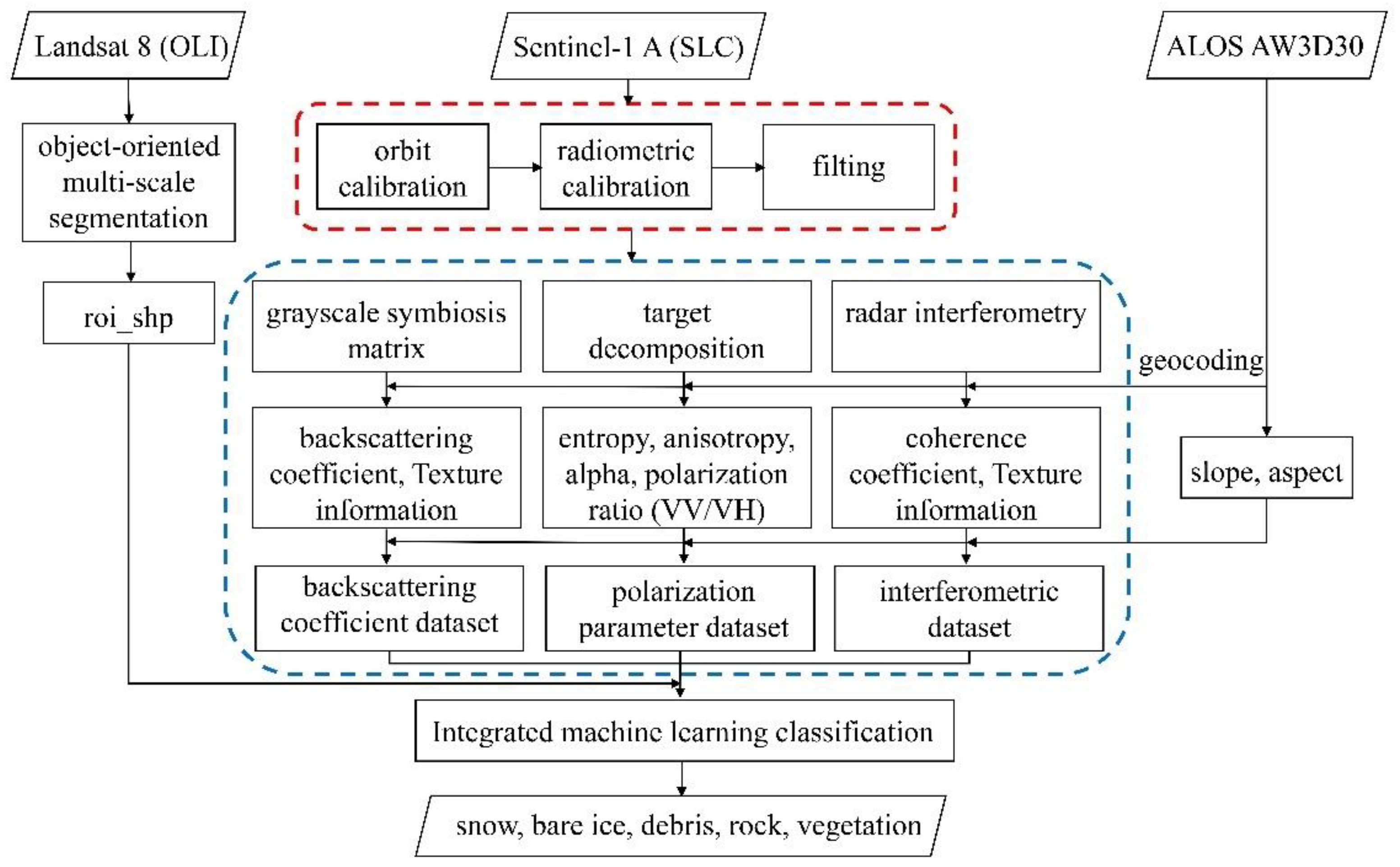
We pre-processed the raw SLC data according to the following procedure. We (1) downloaded the Precise Orbit Ephemerides of Sentinel-1A from the website [61] for orbit calibration, (2) performed radiometric calibration to obtain the backscattering coefficient (sigma naught in dB), and (3) underlay a speckle filter with a refined Lee filter [62] (5 × 5 window size) to eliminate image noise and improve image quality. (4) Orientation angle correction was required prior to polarization decomposition, which allowed for some topographic correction of SAR images by eliminating orientation angle shifts. These steps were completed in the Sentinel Application Platform (SNAP), an open-source ESA toolbox. After the backscattering coefficient data were obtained, three types of processing (see Section 3.1, Section 3.2 and Section 3.3) were performed before the machine learning classification (blue box in Figure 3).

3.1. Target Polarimetric Decomposition

There are not many polarization decomposition techniques for the dual-polarization SAR system, and the most common and mature method is the H/alpha decomposition or H/A/α decomposition in full-polarization decomposition. It originated from the Cloud–Pottier decomposition and was based on an eigenvalue analysis of the coherency matrix T3 to generate estimates of the average target scattering matrix parameters [63]. The advantage of this algorithm is that prior knowledge of the study area is not needed [25].
Dual-polarization decomposition is a special form of full-polarization decomposition. In full-polarization decomposition, the Sinclair matrix [ S f ], scattering vector k _ f , and coherency matrix [ T f ] are obtained by Equations (1)–(3) [64]:
S f = [ S H H S H V S V H S V V ] ,
k _ f = 1 2 [ S H H + S V V S H H S V V 2 S H V ] t
T f = k _ f · k _ f * t
where the subscript f means full-polarization, the superscript t denotes the matrix transpose, and the superscript *t denotes the complex conjugate transpose, 〈…〉 indicates temporal and spatial ensemble averaging.
In the dual-polarization SAR system of Sentinel-1A, under the reciprocity principle, the Sinclair matrix [ S d ], scattering vector k _ d , and coherency matrix [ T d ] all differ from those of full-polarization [65]:
S d = [ 0 S V H S V H S V V ]
k _ d = [ S V V 2 S V H ] t
T d = k _ d · k _ d * t
where the subscript d means dual-polarization. After calculating the eigenvalues and eigenvectors of the coherency matrix, three secondary parameters are obtained:
H = i = 1 2 ( P i log 2 P i )
A = λ 1 λ 2 λ 1 + λ 2
α = i = 1 2 P i α i
P i = λ i / k = 1 2 λ k
where λ i   ( i = 1 ,   2 )   is eigenvalue of the coherency matrix, with λ 1 λ 2   . H is the scattering entropy with values between 0 and 1, denoting the degree of statistical disorder. As for A (anisotropy), in full-polarization, the coherency matrix can be decomposed into three eigenvalues, so its formula is λ 2 λ 3 λ 2 + λ 3 , which indicates the proportion of the second and third scattering components in the entire scattering matrix when the value of H is greater than 0.7 [63]. In the case of dual-polarization, however, the coherency matrix can only be decomposed into two eigenvalues, where the formula of A is λ 1 λ 2 λ 1 + λ 2 , the normalized difference of the 1st and 2nd eigenvalues, which is obviously different from anisotropy, represents the normalized difference of the importance of scattering type, rather than the difference between the second and third scattering components [44]. α is the mean scattering angle (alpha angle) calculated by the weighted average of eigenvectors, with values of 0, π/4, and π/2, representing single-bounce scattering, volume scattering, and double-bounce scattering, respectively. More details on the dual-polarization H/alpha decomposition can be found in [64,65,66,67,68,69].
However, not all dual-polarization can be decomposed. There must be coherent polarimetric radars; otherwise, it is not possible to calculate the off-diagonal elements of the coherency matrix. Moreover, since the scattering matrix of dual-polarization is not complete, the random surface scattering and volume scattering information extracted from a dual-polarization SAR system are limited owing to the absence of cross-polarization and overlap among various scattering mechanisms in the entropy/alpha plane [65]. Therefore, the roughness and moisture effects cannot be separated as easily as in full-polarization. However, dual-polarization still has the potential to separate different types of volume scattering [67].

3.2. SAR Interferometry

Radar interferometry technology uses two single-track dual-antenna observations or single-antenna multiple orbit observations over the same area to form an interferometric pair. There are many factors that cause decoherence, including baselines of observations, elevation, location changes of the same pixel, and all types of noise. The coherence coefficient of a pixel is expressed as the product of several components [68]:
γ = γ o r b + γ t o p o + γ n o i s e + γ a t m o s p h e r e + γ d e f o r m a t i o n
The pixel’s positional change contains the most useful information, and it is also the main source of information used in various coherence-based studies [39,68,69]. In this study, since the time baseline was 12 days and the same sensor allowed us to ignore the spatial baseline difference of different interferometric pairs, we assumed that no other factors caused phase differences in the images except for glacial movement and accumulation or ablation. To use more information, we calculated texture information based on the interferometric coherence coefficients, which is detailed in the next subsection.

3.3. Texture Calculation

The gray level co-occurrence matrix (GLCM) proposed by Haralick et al. [70] is a widely used method to compute second-order texture measures. Many studies have shown that extracting texture information from radar data can effectively improve classification accuracy [71]. Some researchers have investigated the effect of backscatter changes on texture features and the robustness of texture features [72] and filtered out texture features suitable only for specific land surface types [71]. This study used nine different texture features inside three groups (contrast, orderliness, and statistics): Contrast, dissimilarity, homogeneity, angular second moment, energy, maximum probability, GLCM mean, GLCM variance, and GLCM correlation.
The next step was to reduce redundancy among the derived texture information. We overlayed nine texture images (layers) into a “multispectral image” and then used principal component analysis (PCA) to reduce redundancy. After this, the result was still a nine-layer data cube, but the information was concentrated in the first few layers (principal components). In our experiments, the first three layers of the data cube contained nearly 99% of the texture information, so we chose the first three layers to form the three data suites.

3.4. Data Suite Creation

Finally, the backscattering coefficient polarization decomposition parameters, interferometric coherence coefficient, and their respective texture features were combined to generate the three data suites (see Table 2); each contained seven layers. All three suites contained the local incident angle, elevation, and slope as the common layers. The other four layers were the backscattering coefficient (sigma naught); backscattering coefficient-based textures 1, 2, and 3 for the BC suite; entropy, anisotropy, alpha, and VV/VH ratio for the PDP suite; and the coherence coefficient and coherence coefficient-based textures 1, 2, and 3 for the ICC suite, respectively. All preprocessing and information extraction were carried out in SNAP.
Since data from ascending (A) and descending (D) orbit nodes were used and Sentinel-1A had two polarization imaging modes (VV and VH), four data suites were formed for the BC and ICC suites based on the orbit node and polarization mode: Ascending co-polarization (A_VV), ascending cross-polarization (A_VH), descending co-polarization (D_VV), and descending cross-polarization (D_VH). However, for the PDP suite, polarization decomposition required two polarization data sources simultaneously, so only two data suites for PDP were formed: Ascending and descending PDP suites.

3.5. Integrated Machine Learning Method

The classifier is critical for classification accuracy. Machine learning algorithms have been fully applied and popularized in remote sensing research [73,74,75], especially for image classification and target change detection [76,77,78,79].
This study used the Classification Learner module in MATLAB R2020a software to perform the machine learning classification. The module included multiple classifier classes, but we only focused on four: Decision trees (Tree), support vector machine (SVM), k-nearest neighbor (KNN), and ensemble. Table 3 lists the 20 algorithms inside these four classifier classes.
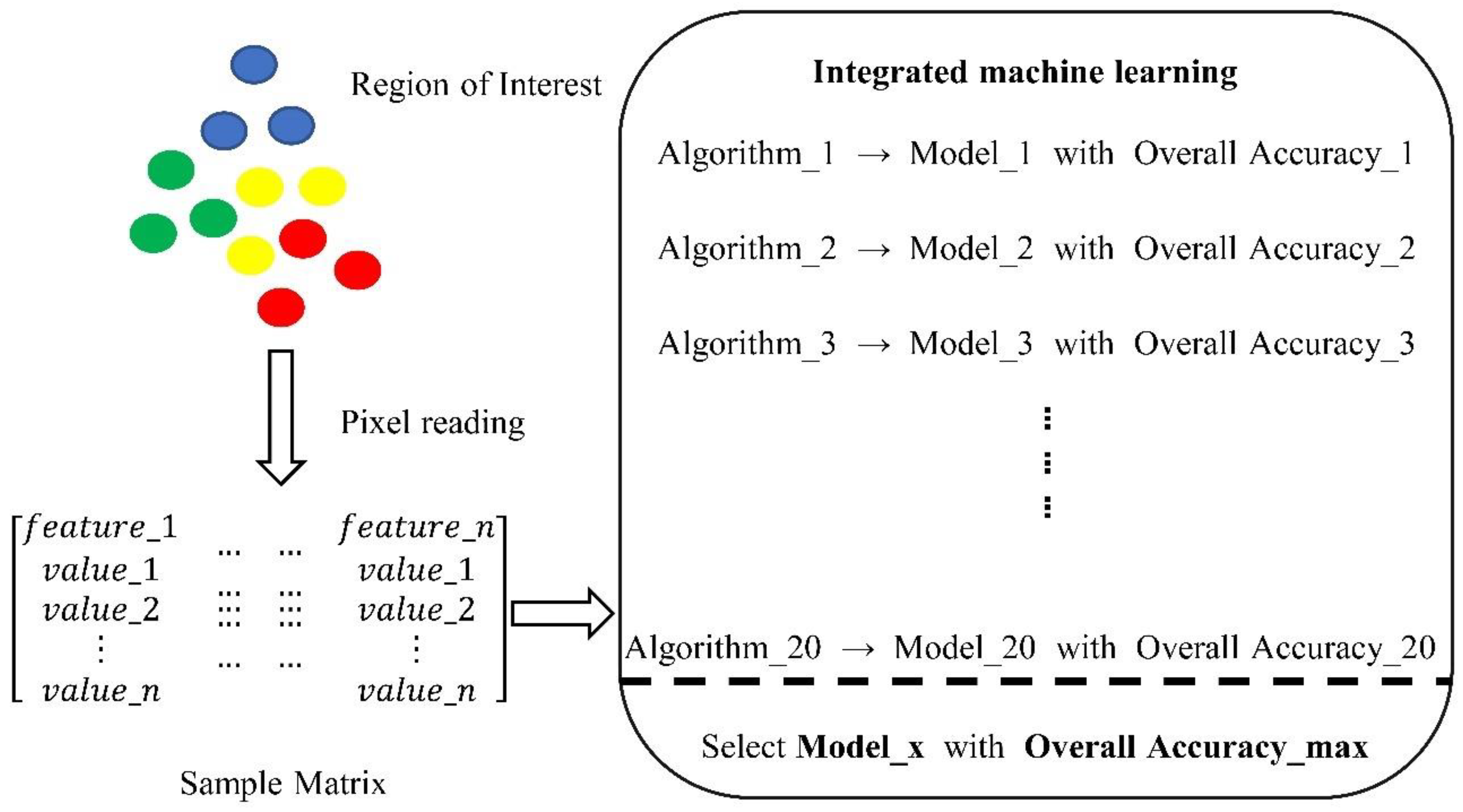
The samples of various land surface types were read as a matrix and imported into the integrated machine learning classification. As Figure 3 shows, the vector boundaries (shapefile roi_shp) of the regions of interest (ROIs) were obtained from the Landsat 8 optical images after segmentation. Each glacier had an ROI shapefile containing five surface types: Snow, bare ice, debris, rock, and vegetation. We used the shapefile to clip the data suites. In particular, the NW and NE glaciers’ optical images did not show any vegetation near the glacier, so there were only four land surface types for these images. The number of sample pixels for each land surface type for each glacier exceeded 1000; 70% of the pixels were used as training samples, and the remaining pixels were used to evaluate classification accuracy.
Every sample matrix for each glacier was input into the integrated machine learning classification process to produce 20 sets of results and 20 trained models from the 20 classification algorithms. Each model had a predicted classification accuracy. The classification models with the highest prediction accuracy were selected as the optimized models to classify new data suites (Figure 4).

3.6. Feature Importance Calculation

The Kruskal–Wallis test is a nonparametric test comparing multiple independent samples and creating a ranking, accompanied by a p-value to help explain reliability. In this study, we used the Diagnostic Feature Explorer tool [80] in MATLAB to perform the Kruskal–Wallis test and rank the importance of all features for each data suite. This consisted of three steps. First, the samples of all glaciers in each data suite were read as a matrix of n × 8; the first seven columns corresponded to the seven layers in each data suite, and the last column was the label for the land surface type. Each row corresponded to a sample for a total of n rows. Then, three matrices were generated corresponding to the BC, PDP, and ICC data suites. Second, the Kruskal–Wallis test was performed for each feature in the matrix. Last, a chi-square statistical analysis was performed on the results from the second step, which were outputs from the analysis of feature ranking and the score for each feature in the matrix, where a larger score value indicated the higher importance of the corresponding feature. We then determined the importance of all features of the three types of data suites in the classification process based on the returned score value.

3.7. Aspect-Beam Angle

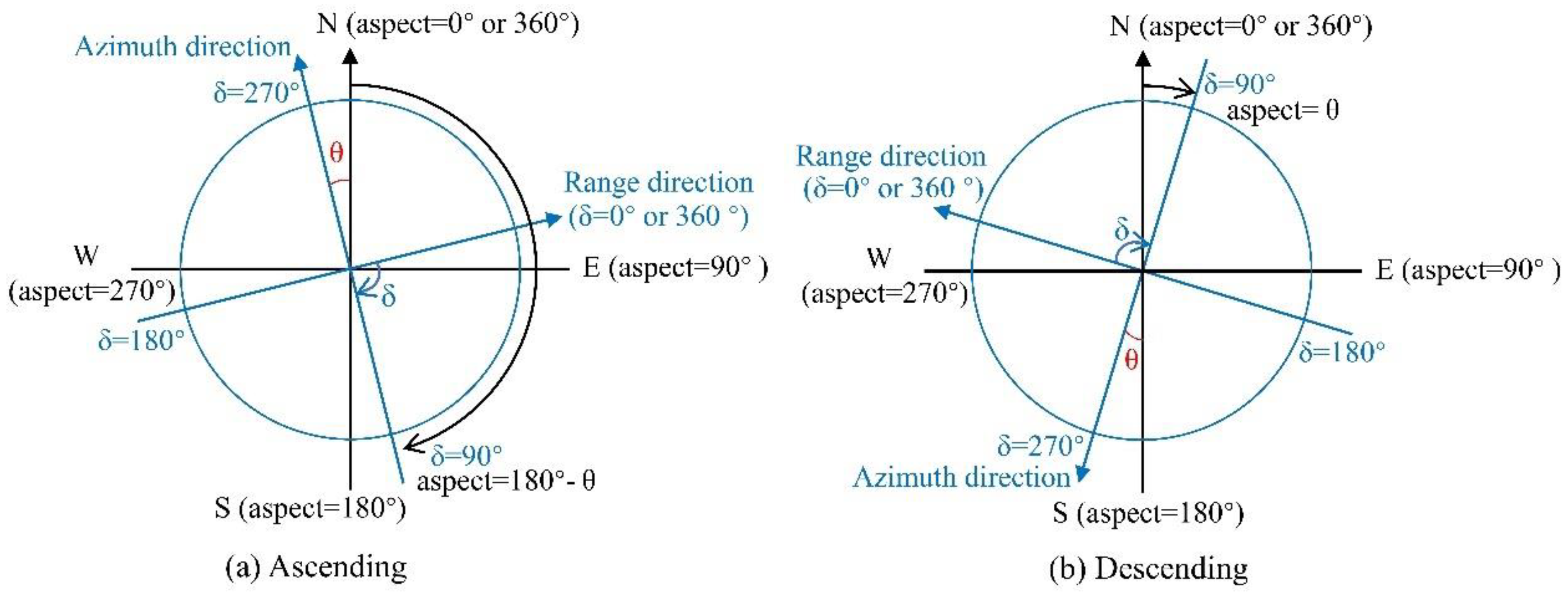
Terrain is an unavoidable influencing factor for microwave remote sensing in mountainous areas. In addition to shadowing and overlay masking, the terrain also alters the backscattering, which affects the subsequent feature extraction. In this regard, we introduced a new parameter to assist in evaluating the influence of the terrain of the glacier area on the glacier identification accuracy. The aspect-beam angle (δ) is defined as the angle between the radar beam’s propagation direction and the aspect of a pixel, ranging from 0 to 360 degrees, where the pixel aspect is calculated from the DEM data and indicates the orientation of the glacier surface at the pixel level.
As Figure 5 shows, when the pixel’s aspect was in the same, right vertical, opposite, and left vertical state with the incident radar beam direction, δ was 0, 90, 180, and 270 degrees, respectively. This transformation reduced the three-dimensional spatial relationship between the ground surface and the radar antenna to two dimensions and divided it into four ranges:
  • S (small): δ values ranging from 0 to 45 degrees and 315 to 360 degrees, representing total forward scattering;
  • M (medium): δ values ranging from 45 to 135 degrees and 225 to 315 degrees, with the former called M_r and the latter called M_l, since they are located on the right and left sides of the direction of the radar beam propagation; they both represent a mixture of forward and backscattering scattering;
  • L (large): δ values ranging from 135 to 225 degrees, representing total backscattering.
Based on the above four aspect-beam angle ranges, three secondary statistical quantities are defined by Equations (12)–(14):
PD_V = M_r + M_l,
SD_H = ABS (M_r − M_l),
SD_V = ABS (S − L)
where SD is short for symmetrical degree, PD is short for primary direction, V indicates vertical to the radar beam direction, H indicates parallel to the radar beam, ABS is the absolute value of the difference; these three secondary statistical characteristics all take values between 0 and 100, where a larger value of PD_V indicates that the glacier surface tends to be perpendicular to the radar beam direction, and vice versa. SD_H indicates the symmetry of the glacier aspect about the plane parallel to the radar beam’s direction. The smaller the value, the better the symmetry, and vice versa. Similarly, SD_V indicates the symmetry of the glacier aspect about the plane perpendicular to the radar beam’s direction, and the smaller the value, the better the symmetry, and vice versa.

4. Results

4.1. Aspect-Beam Angle in Four Glaciers

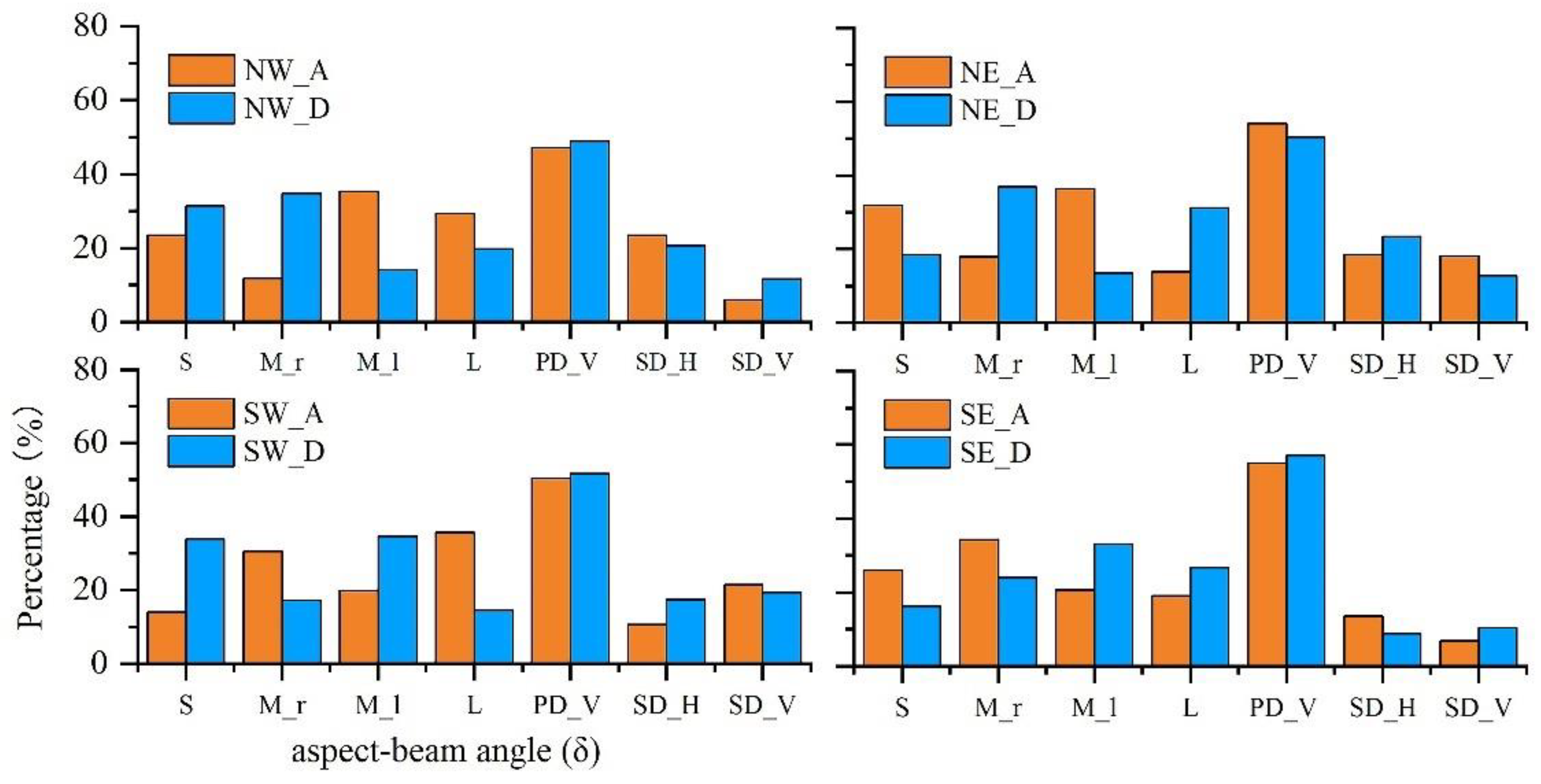
According to the method described in Section 3.7, we obtained the aspect-beam angle of the four glaciers and then counted the proportion of the four sub-ranges (S, M_r, M_l, and L) in each glacier and the values of the three secondary statistical parameters (PD_V, SD_H, SD_V); their histograms under ascending and descending nodes are shown in Figure 6.
As for the distribution of the aspect-beam angle values in the four sub-ranges, in the NW glacier, they were mainly distributed in the M-left and L ranges, for images of the ascending node and S and M-right ranges, respectively, for images of the descending node, as expected. For the NE glacier, they were mainly distributed in the S and M-left ranges, for images of the ascending node and M-right and L ranges, respectively, for images of the descending node, also as expected. For the SW glacier, they were mainly distributed in the M-right and L ranges, for images of the ascending node and S and M-left ranges, respectively, for images of the descending node. For the SE glacier, they were mainly distributed in the S and M-right ranges, for images of the ascending node and M-left and L ranges, respectively, for images of the descending node. In addition, the cumulative differences between the four ranges of each glacier in different orbital directions, in descending order, occurred in the NE, SW, NW, and SE glaciers, indicating that the SE glacier was the least influenced by the sensor orbital direction and NE was most influenced.
Among the three secondary statistical parameters, the values of PD_V were taken from the SE, NE, SW, and NW glaciers in descending order, indicating that most of its surface area was oriented parallel to the radar beam, while the remaining three glaciers were the opposite. The values of SD_H were taken from SE, SW, NE, and NW in descending order, and SD_V was taken from SE, NW, NE, and SW in descending order. The values of these two ranges implied that the SE glacier had the best symmetry, both parallel and perpendicular to the radar beam plane, with NW having more pronounced symmetry about the sensor orbital plane, while the glacier surface aspect symmetry of both NE and SW glaciers was weaker, and the difference between them was that the former tended to be more symmetric about the orbital plane and the latter tended to be more symmetric about the radar beam plane.

4.2. Machine Learning Classification Models

We obtained the prediction accuracy for 20 machine learning models from the three types of data suites for the four glaciers through the integrated machine learning classification algorithms. Among the four classifier classes, the SVM classifier class had the highest average accuracy (84.63%), followed by the ensemble classifier class (83.40%), tree classifier class (82.90%), and KNN classifier class (80.84%). The best classification accuracies from training using the four classifier classes for the four glaciers are shown in Figure 7a: The average prediction accuracy of all classifier classes for the NW glacier was the best (94.61%), followed by the NE glacier (89.64%), the SE glacier (86.35%), and the SW glacier (61.15%).
Figure 7b shows the prediction accuracy for the four glaciers from each of the 20 algorithms (see Table 3). For the tree classifier class, the average accuracy of its three algorithms for the four glaciers was between 60.73 and 96.64%, with a standard deviation of 13.04%. For the SVM classifier class, the average accuracy of its six algorithms was between 59.01 and 96.35%, with a standard deviation of 12.91%. For the KNN classifier class, the average accuracy of its six algorithms was between 51.12 and 94.53%, with a standard deviation of 14.81%. For the ensemble classifier class, the average accuracy of its five algorithms was between 55.32 and 97.30%, with a standard deviation of 15.66%.
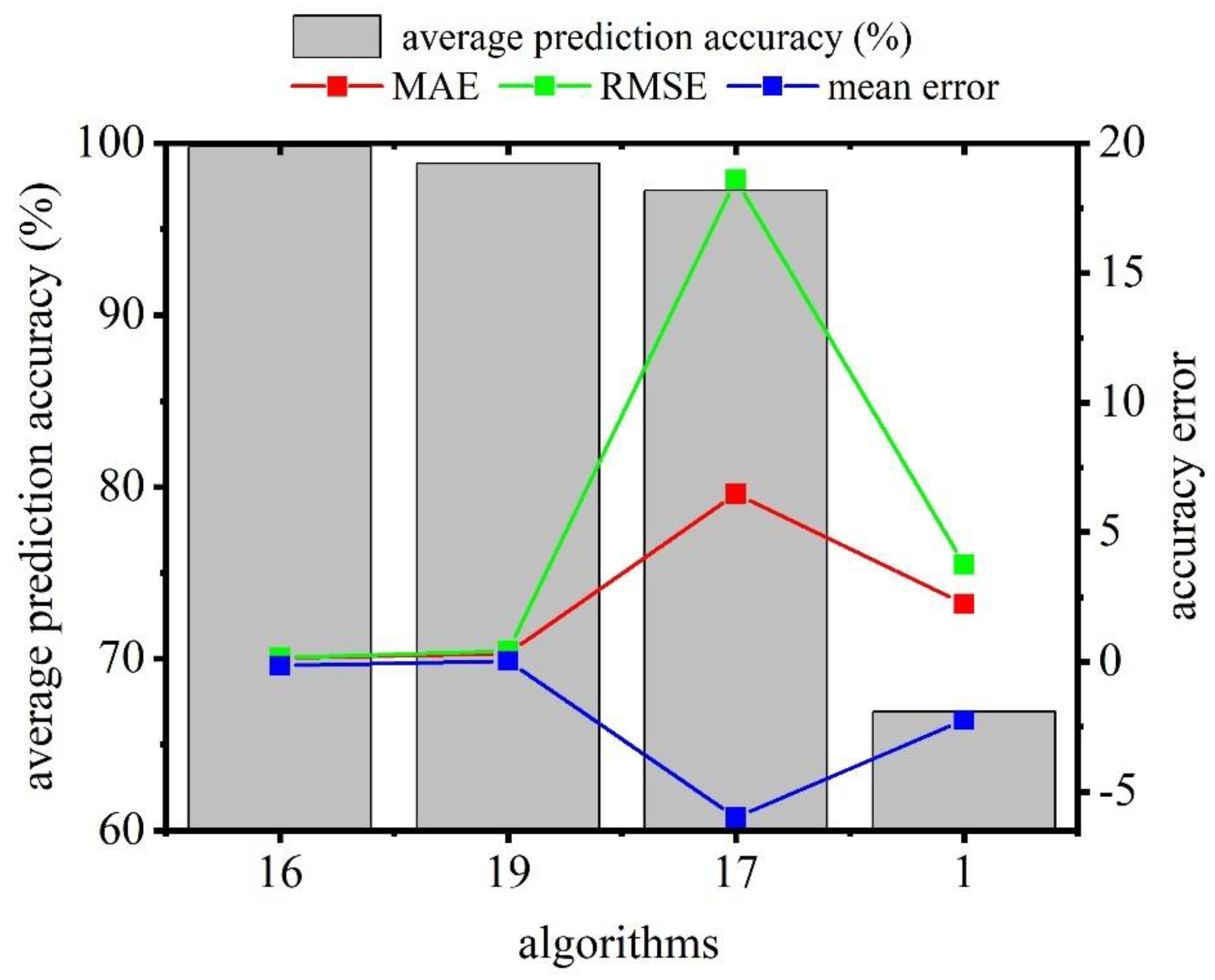
From the above analysis, the optimal classification model for each glacier was filtered: They include boosted trees, bagged trees, and subspace KNN for the ensemble classifier class and fine tree from the decision trees class. After performing the classification to determine the actual classification accuracy, we calculated the error between it and the prediction accuracy and further analyzed the effectiveness of these four algorithms using three commonly used quantitative algorithm quality metrics: Mean absolute error (MAE), root mean square error (RMSE), and mean error (Figure 8).
In Table 4, the first column is the glaciers, the second column is the selected algorithm with the highest classification accuracy, and columns 3–5 correspond to the three data suite categories, including all possible data suites in each category considering the orbit nodes and polarization modes. Each row represents the actual classification accuracy corresponding to each algorithm from different data suites, where error means the difference between the actual and predicted classification accuracies. A positive error value indicates that the actual classification accuracy is higher than the predicted accuracy and vice versa. The classification accuracy of these four models for all data suites ranged from 41.70 to 99.94%, and the error between them and the prediction accuracy ranged from –56.64 to 0.74%. Among them (Figure 8), the boosted trees and subspace KNN algorithms achieved the best classification accuracy in the actual classification with the smallest MAE and RMSE. Although the bagged trees also had high classification accuracy, the actual classification could not reach the optimal result, and the MAE and RMSE were large. For the fine trees, the classification accuracy was relatively low. Based on these results, we found that the boosted trees and subspace KNN algorithms were the best machine learning classification models with high accuracy and good robustness.

4.3. Classification Results from Different Data Suites

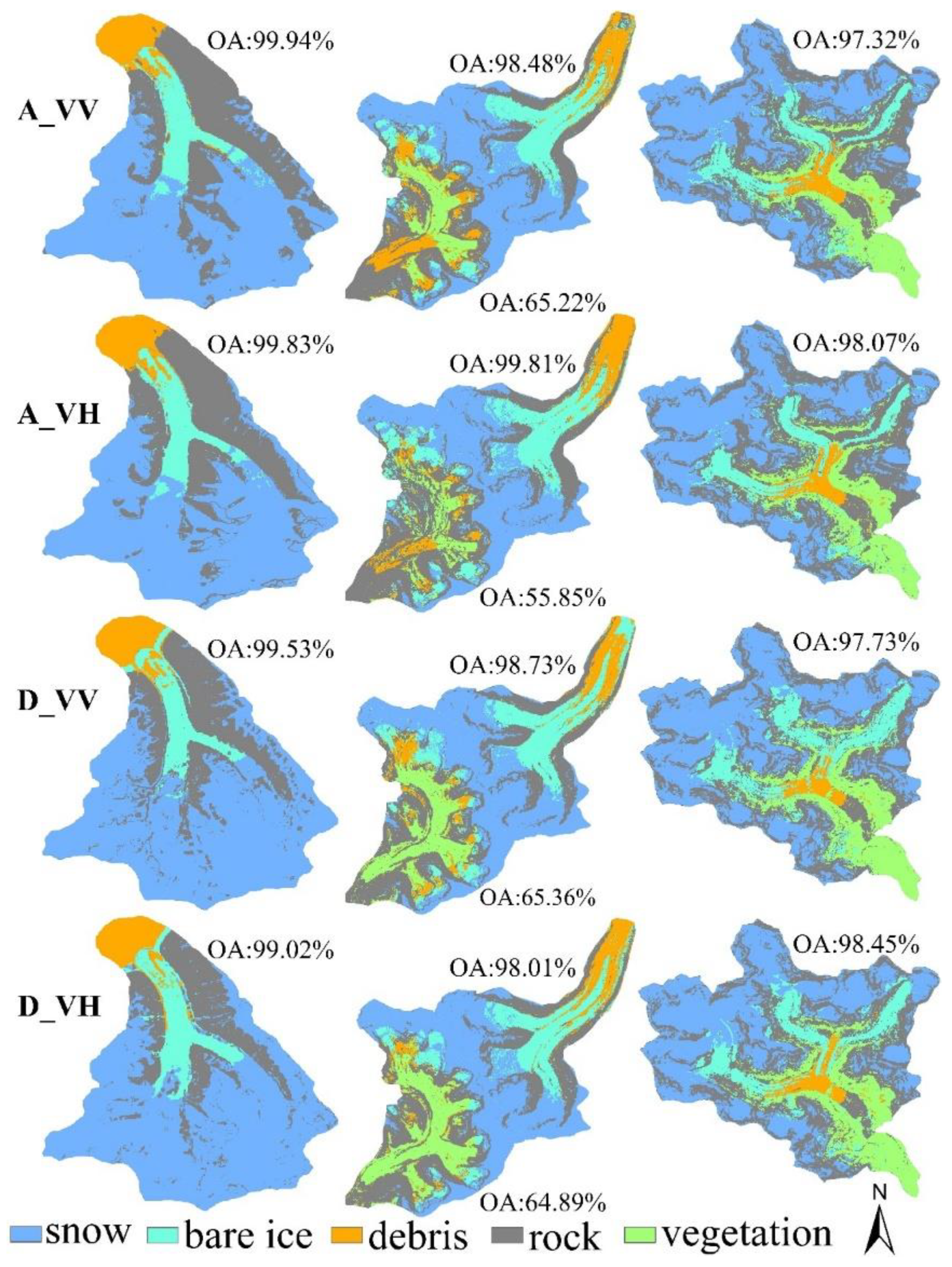
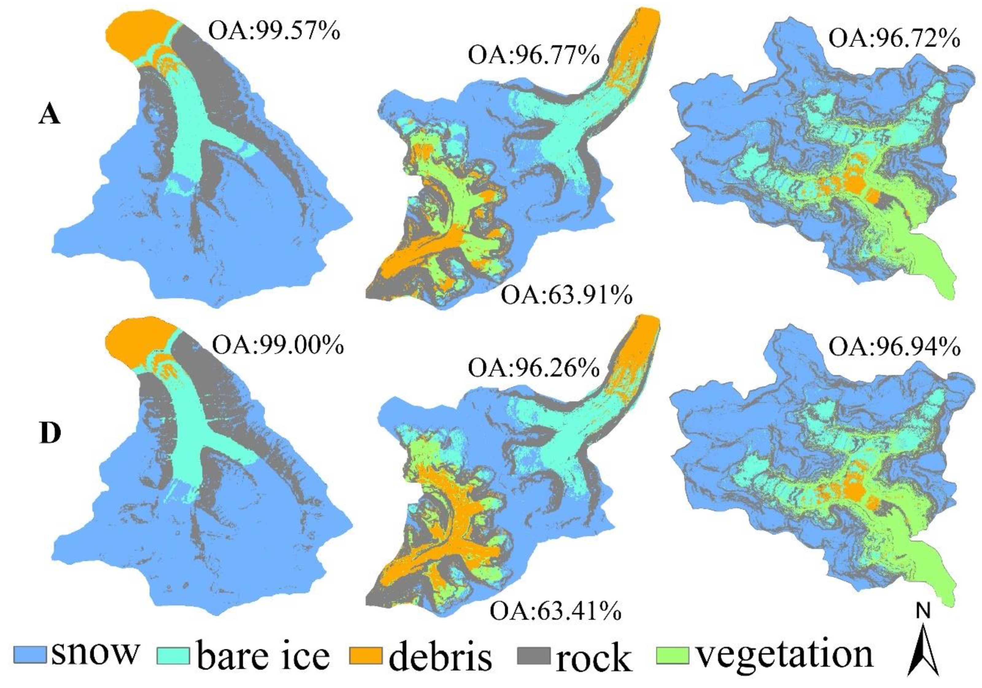
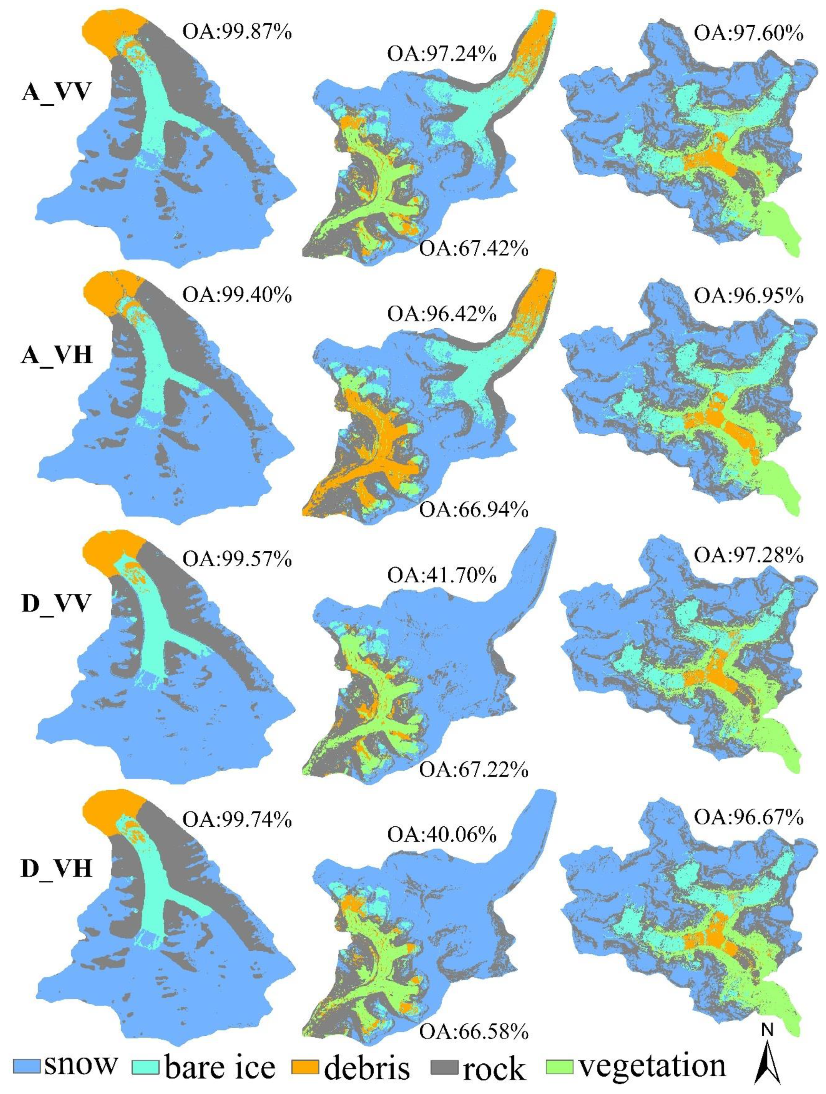
The false-color images of the classification results from the BC, PDP, and ICC data suites for each glacier are shown in Figure 9, Figure 10 and Figure 11.
For the BC data suite category, the overall accuracy (OA) of the four glaciers from the four data suites ranged from 55.85 to 99.94%, with a mean of 89.70%; specific to each glacier, the OA of the NW, NE, and SE glaciers was better than 97% in all four data suites. In contrast, the SW glacier had less than 65.36% accuracy. The different land surface types in descending order of recognition accuracy were snow (97.69%), rock (93.87%), bare ice (90.14%), debris (83.53%), and vegetation (72.19%). Further analysis of the confusion matrix combined with the false-color images of classification results (Figure 9) revealed that the largest percentage of misclassification occurred among the vegetation, bare ice, and debris surface types, causing a low OA for the SW glacier.
The OA of the four glaciers in the two data suites of the PDP data suite category ranged from 63.41 to 99.57%, with a mean of 89.07%. Among the four glaciers, the OA of the NW, NE, and SE glaciers was better than 96% in all the data suites, while the SW glacier had an accuracy of less than 63.91%. Land surface types are listed in descending order of recognition accuracy as follows: Snow (97.31%), rock (95.34%), bare ice (89.83%), debris (83.14%), and vegetation (69.52%). The false-color diagrams and confusion matrix of classification results (Figure 10) revealed that the low OA of the SW glacier was still caused by the misclassification of debris and vegetation, but it was better than that of the BC data suites in descending node.

5. Discussion

5.1. Importance Analysis of Features

To investigate the different roles of layers in each data suite during the classification, cross-correlation analysis and relative importance ranking for each data suite’s layers were performed.
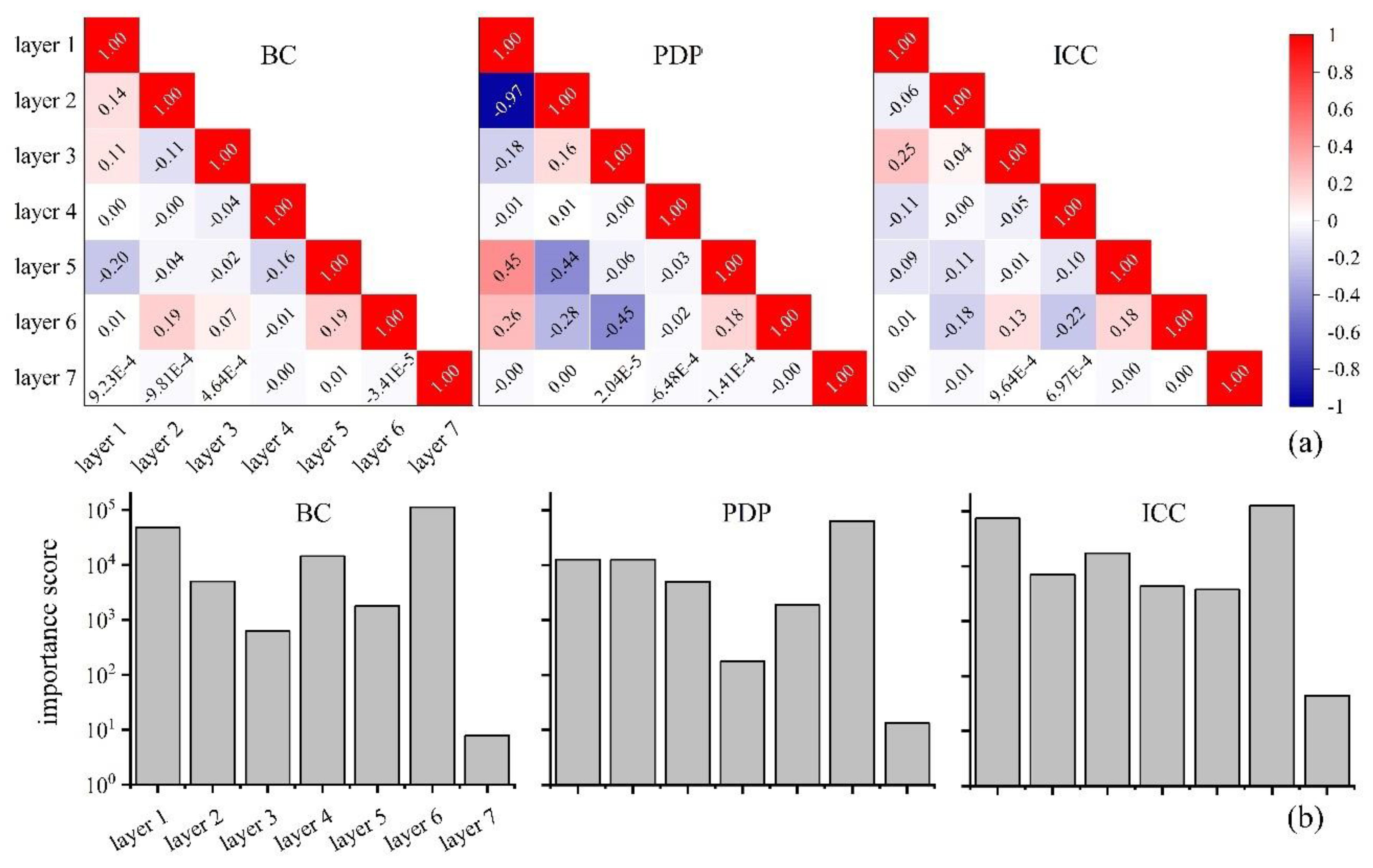
As shown in the heat map of Figure 12a, the abscissa and ordinate correspond to layers 1–7 of each data suite, and the colors from red to blue range from a strong positive correlation to a strong negative correlation. For the BC suite, the Pearson correlation coefficient between any two of the seven layers was between −0.2 and 0.19. For the PDP suite, the correlation coefficient ranged from −0.97 to 0.45. In the ICC suite, the correlation coefficient ranged from −0.22 to 0.25. Among the three data suite categories, the correlation between any two layers in each data suite was not significant, except for the high cross-correlation between layer 1 and layers 2 and 5 in the PDP suite, which were the entropy and anisotropy from the H/alpha decomposition, respectively. This high cross-correlation implied that redundancy reduction can be achieved by retaining entropy instead of both in future studies.
Through the method described in Section 3.6, each layer’s importance was calculated and sorted using the classification accuracy as a variable (Figure 12b). It was clear that glacier elevation was the most important topographic parameter in all three data suite categories, followed by layer 5, which was the local incident angle. These results were consistent with previous studies [23,40,41,45]. The slope was unexpectedly less important, probably because the difference in slope among the various land surface types in the four glaciers was not significant and therefore did not appear to contribute. The importance ranking of the layers related to radar information varied among the three data suites. Between the BC and ICC suites, the backscatter coefficients as well as the interferometric coherence coefficients were more important than the respective texture information, while in the PDP suite, the three polarization decomposition features had similar importance, but the polarization ratio was less important.

5.2. Impact of Data Suite on Glacier Identification

The differences among the three data suites were mainly manifested in the following three aspects: Composition structure, importance ranking, and robustness of classification effect.
Regarding the difference in composition structure, the first four layers of each suite comprised information from radar images, and the remaining three layers were from topographic data. In the BC suite, the radar information was sigma naught, which was very sensitive to the differences in the physical properties of land surface, especially the surface roughness closely related to elevation distribution [39]. The texture information derived from sigma naught further strengthened this difference. Therefore, the bare ice and debris inside the glacier were well recognized. In the PDP suite, the first four layers were the polarization decomposition parameters and the polarization ratio. The decomposed polarization features were used to determine the complexity of the scattering mechanism, the component of the non-primary scattering mechanism, and the mean scattering angle. Compared with the backscattering coefficients, these secondary statistical features appeared to be more advanced, especially the scattering mechanisms corresponding to the mean scattering angle, which were superior in distinguishing the debris from rocks and snow of different densities. Therefore, the PDP suite is recommended for debris-covered glaciers. In the ICC suite, the first four layers were the radar interference coherence coefficient and its texture information. The interference coherence coefficient is a parameter that reflects the similarity of the same pixel during two observations so that it will be affected by glacier movement. This parameter is more dynamic, and its advantage is that it can distinguish the glacier from the surrounding rocks, but when the glacier moves or changes quickly, it will lose coherence, making it difficult to identify the glacier effectively [81]. In this study, the data acquisition time of the descending data was 3 days later than that of the ascending data, which was close to the end of the ablation season. We speculated that this caused the coherence coefficient to decrease, which in turn led to an abrupt decrease in the glacier classification accuracy of the descending nodes of the ICC suite.
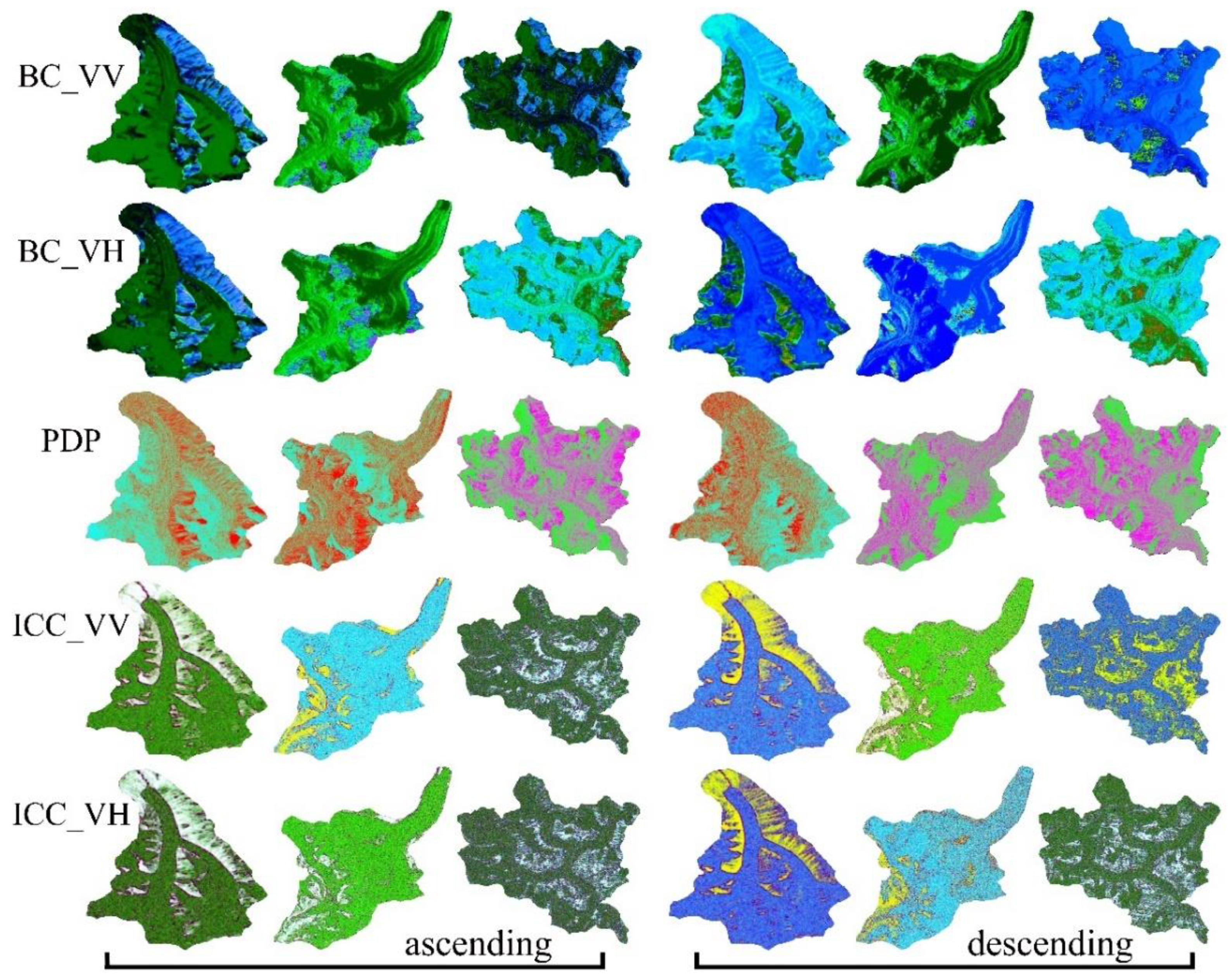
According to the importance sorting, we selected the first three most important layers in each data suite for false-color display (Figure 13). In the BC and PDP suites’ false-color images, the pixel brightness for ascending and descending orbits was symmetrical. This symmetry phenomenon was not found in the ICC suite, which had only some color change owing to R, G, B channel ratio changes. This mainly was because the spatial relationship between the antenna and the glacier surface changed only slightly during interferometry so that the coherence coefficient could be calculated to avoid complete decoherence in the ascending or descending images. Thus, the BC suite and PDP suite were more sensitive to sensor orbital direction than the ICC suite.
As designed, each data suite category had two or four data suites, depending on the orbital direction or polarization. However, according to Figure 11, we found that within each data suite, the effect of extracting glaciers or the accuracy of identifying land surface type was different. Taking the NE glacier as an example, the ICC suite’s OA did not reach 45% for the descending images; debris and bare ice were all misclassified as snow, which was much worse than the BC and PDP suites or even the ICC suite for ascending images. Considering that we used the same classification algorithm and the sample boundary in the ascending and descending data suites in the ICC suite category for the NE glacier, the only difference was the training samples’ pixel values. Since the ICC suite was not as sensitive to orbital direction as the BC and PDP suites, the only possibility may be that the interferometric coherence coefficients of the descending images changed and were not as favorable for glacier classification as the ascending images. Thus, the BC and PDP suites had better performances in identifying various glaciers and land surface types.

5.3. Impact of Glacial Aspect on Recognition

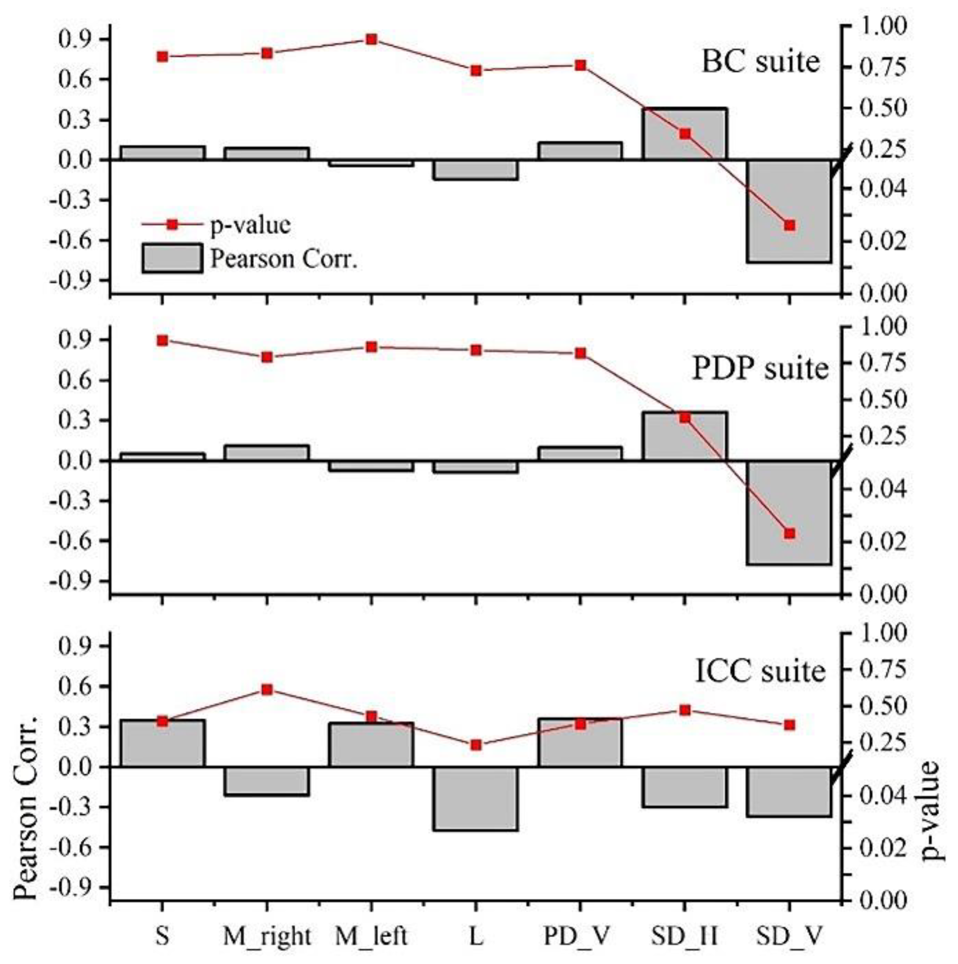
This section analyzes how the glacier aspect distribution affected the glacier identification accuracy based on the results from Section 4.1 and Section 4.3. Figure 14 shows the Pearson correlation coefficients and p-values between the glacier surface aspect-beam angle ranges and the glacier classification accuracy from the three data suite categories and their probabilities. It was found that the Pearson correlation coefficients were less than 0.5 and the p-values were greater than 0.05, indicating that there was no significant correlation between the four aspect-beam angle ranges and glacier identification accuracy. Among the three secondary statistical parameters (Equations (12)–(14)), only SD_V showed a p-value less than 0.05, with a Pearson correlation coefficient less than −0.6, indicating SD_V was negatively correlated with classification accuracy. This may imply that pixels with smaller SD_V values were identified with high classification accuracy. In other words, the glacier surface aspect that was more symmetrical about the sensor orbital plane was identified with higher accuracy. This significant negative correlation only occurred in the BC and PDP suites, which indicated again that the BC and PDP suites were more sensitive to the sensor orbital direction. On the other hand, it may also indicate that the glacier surface aspect had a limited role in identifying glaciers from the ICC data suite. A glacier can be divided into different subregions according to the S, M, and L ranges, or we can select satellite images with different orbital aspects from multi-angle observations to compensate for the negative correlation in the BC and PDP data suites. Sample selection, model training, and classification can be performed separately for each subregion to improve the accuracy of classification.
On the other hand, the main aspects of the NE and SW glaciers were more parallel to the radar beam direction than the other two glaciers, but the classification accuracy for the NE glacier was much higher than that for the SW glacier. By further comparing the elevation and slopes of the two glaciers (see Figure 2), we found that the NE glacier reached 2000 m in elevation and the SW glacier reached 3000 m. Furthermore, the NE glacier had a significantly higher pixel proportion than the SW glacier within a slope value of less than 15 degrees over that with a slope value above 15 degrees, or the NE glacier was relatively much gentler in slope than the SW glacier, thus improving the accuracy. Therefore, we speculate that the low recognition accuracy of SW glaciers in many data suites was due to the fact that there were more steep slopes inside the glaciers, which formed more electromagnetic wave disturbances and reduced the interpretability of the returned electromagnetic waves.

5.4. Uncertainties and Possible Transferability Analysis

The main contribution of this study was to compare the effectiveness of three mainstream radar information sources in identifying debris-covered alpine glaciers with full consideration of the topographic features. The highest accuracy was not our ultimate goal, so there are some shortcomings to the study, such as the failure to consider the combination of radar and optical data and thermal data, which are beneficial for glacier identification according to previous studies [82,83,84]; thus, combining these data on the basis of this study should lead to better identification results. In addition, classical machine learning algorithms were chosen, and training samples were manually labeled that were not as smart as deep learning algorithms but still achieved satisfactory results with a limited training data set.
In the design of the radar information-based data suites, the dual-polarized Sentinel-1A data limits the choice of polarization decomposition parameters, especially compared to the fully polarized SAR data [26], which allows for more decomposition features, resulting in a PDP suite that enables more differentiation of land classes in glaciated areas and obtains higher accuracy.
Furthermore, radar wavelength was highly important in the interferometric process. The data in the C-band were chosen to have comparability between different data suites, and other bands may have had different effects, such as the L-band obtaining stronger penetration, interference coherence, and polarization capabilities because of its longer wavelength [85].

6. Conclusions

In this study, four glaciers with different aspects in the TP were selected as research sites, and three types of data suites were developed in combination with Sentinel-1A SLC data and topographic data: The BC suite, the PDP suite, and the ICC suite. They represented the three main types of radar information: The backscattering coefficient, polarization decomposition parameters, and the interference coherence coefficient, respectively. After sample selection with the aid of Landsat 8 OLI, an integrated machine learning classification method was used to select the optimal classification model and perform classification. Finally, the importance of each data layer within a data suite in glacier identification, the impact of the type of data suite, and the glacier aspect on the classification accuracy were compared and analyzed.
We conclude the following: (1) In all data suites, the elevation was the most important parameter affecting the accuracy of glacier identification, and the aspect-beam angle was the secondary important topographic parameter. In the BC and ICC suites, the secondary important factors were the backscatter coefficient and the interferometric coherence coefficient, respectively, while in the PDP suite, there were no particularly prominent radar parameters. (2) Both BC and PDP suites achieved robust and very high classification accuracy, especially the PDP suite, which was better than the BC suite at recognizing debris and rock. Therefore, it is recommended to identify debris-covered glaciers. Although the ICC suite achieves similar accuracy, it is not recommended for fast-moving glacier areas owing to its sensitivity to glacier movement speed. (3) The ICC dataset was less influenced by the directional features of the glacier surface, while the BC and PDP datasets were more influenced; the more symmetrical the glacier surface was about the sensor orbital plane, the more favorable the recognition. In addition, a small glacier slope was favorable for identification and vice versa. Therefore, the PDP suite is proposed for debris-covered alpine glacier identification and dividing the glacial area into different subdivisions according to the aspect-beam angle to perform the classification process separately, including selecting samples and training different models.

Author Contributions

Conceptualization, G.Y., X.Z. and C.K.; methodology, G.Y. and X.Z.; software, G.Y.; validation, G.Y. and L.D.; formal analysis, G.Y.; data curation, G.Y.; writing—original draft preparation, G.Y.; writing—review and editing, X.Z., C.K. and H.L.; visualization, G.Y.; funding acquisition, C.K. and H.L. All authors have read and agreed to the published version of the manuscript.

Funding

This work was supported by the National Natural Science Foundation of China (grant no. 41830105, no. 41301611).

Data Availability Statement

The data presented in this study are available on request from the corresponding author.

Acknowledgments

We would like to thank the teams from ESA for providing free Sentinel-1A data and open-source SNAP software, as well as the USGS and JAXA for making their data sets publicly available.

Conflicts of Interest

The authors declare no conflict of interest. The funders had no role in the design of the study; in the collection, analyses, or interpretation of data; in the writing of the manuscript, or in the decision to publish the results.

Abbreviations

List of Main Abbreviations and Their Explanations (Alphabetical Order)
A_VHThe VH polarization mode under the ascending node
A_VVThe VV polarization mode under the ascending node
BCBackscattering Coefficient
D_VHThe VH polarization mode under the descending node
D_VVThe VV polarization mode under the descending node
GLCMGray level co-occurrence matrix
ICCInterference Coherence Coefficient
KNNK-nearest neighbor
LThe angle between glacier surface orientation and radar beam propagation direction is between 135–225 degrees
MThe angle between glacier surface orientation and radar beam propagation direction is between 45–135 degrees or 225–315 degrees, the former is also called M_r, the latter is called M_l
NEOne of the four study sites, located in the middle of the Himalayas, the main orientation of the glacier is northeast
NWOne of the four study sites, located in the northwestern part of the TP, the main orientation of the glacier is northwest
OAOverall Accuracy
PDPPolarization Decomposition Parameter
PD_VPercentage of the glacier surface orientation perpendicular to the radar beam direction
SThe angle between glacier surface orientation and radar beam propagation direction is between 0–45 degrees or 315–360 degrees
SD_HSymmetry of the glacier surface orientation with respect to the plane parallel to the radar beam direction.
SD_VSymmetry of the glacier surface orientation with respect to the plane perpendicular to the radar beam direction.
SEOne of the four study sites, located in the southeast part of the TP, the main orientation of the glacier is southeast
SLCSingle-Look Complex
SVMsupport vector machine
SWOne of the four study sites, located in the middle of the Himalayas, the main orientation of the glacier is southwest
TPQinghai-Tibet Plateau

References

  1. Cao, S.X.; Zhang, J.Z. Political risks arising from the impacts of large-scale afforestation on water resources of the Tibetan Plateau. Gondwana Res. 2015, 28, 898–903. [Google Scholar] [CrossRef]
  2. Kääb, A.; Berthier, E.; Nuth, C.; Gardelle, J.; Arnaud, Y. Contrasting patterns of early twenty-first-century glacier mass change in the Himalayas. Nature 2012, 488, 495–498. [Google Scholar] [CrossRef] [PubMed]
  3. Immerzeel, W.W.; Van Beek, L.P.H.; Bierkens, M.F.P. Climate change will affect the Asian Water Towers. Science 2010, 328, 1382–1385. [Google Scholar] [CrossRef] [PubMed]
  4. Bojinski, S.; Verstraete, M.; Peterson, T.C.; Richter, C.; Simmons, A.; Zemp, M. The Concept of Essential Climate Variables in Support of Climate Research, Applications, and Policy. Bull. Am. Meteorol. Soc. 2014, 95, 1431–1443. [Google Scholar] [CrossRef]
  5. Zemp, M.; Huss, M.; Thibert, E.; Eckert, N.; McNabb, R.W.; Huber, J.; Barandun, M.; Machguth, H.; Nussbaumer, S.U.; Gärtner-Roer, I.; et al. Global glacier mass changes and their contributions to sea-level rise from 1961 to 2016. Nature 2019, 568, 382–386. [Google Scholar] [CrossRef]
  6. Tapponnier, P.; Zhiqin, X.; Roger, F.; Meyer, B.; Arnaud, N.; Wittlinger, G.; Jingsui, Y. Oblique Stepwise Rise and Growth of the Tibet Plateau. Science 2001, 294, 1671–1677. [Google Scholar] [CrossRef]
  7. Molnar, P.; Boos, W.R.; Battisti, D.S. Orographic Controls on Climate and Paleoclimate of Asia: Thermal and Mechanical Roles for the Tibetan Plateau. Annu. Rev. Earth Planet. Sci. 2010, 38, 77–102. [Google Scholar] [CrossRef] [Green Version]
  8. Wijngaard, R.R.; Steiner, J.F.; Kraaijenbrink, P.D.A.; Klug, C.; Adhikari, S.; Banerjee, A.; Pellicciotti, F.; Van Beek, L.P.H.; Bierkens, M.F.P.; Lutz, A.F.; et al. Modeling the Response of the Langtang Glacier and the Hintereisferner to a Changing Climate Since the Little Ice Age. Front. Earth Sci. 2019, 7, 143. [Google Scholar] [CrossRef]
  9. Kääb, A. Combination of SRTM3 and repeat ASTER data for deriving alpine glacier flow velocities in the Bhutan Himalaya. Remote Sens. Environ. 2005, 94, 463–474. [Google Scholar] [CrossRef]
  10. Racoviteanu, A.E.; Williams, M.W.; Barry, R.G. Optical Remote Sensing of Glacier Characteristics: A Review with Focus on the Himalaya. Sensors 2008, 8, 3355–3383. [Google Scholar] [CrossRef] [Green Version]
  11. Rabatel, A.; Dedieu, J.-P.; Vincent, C. Using remote-sensing data to determine equilibrium-line altitude and mass-balance time series: Validation on three French glaciers, 1994–2002. J. Glaciol. 2005, 51, 539–546. [Google Scholar] [CrossRef] [Green Version]
  12. Alifu, H.; Vuillaume, J.-F.; Johnson, B.A.; Hirabayashi, Y. Machine-learning classification of debris-covered glaciers using a combination of Sentinel-1/-2 (SAR/optical), Landsat 8 (thermal) and digital elevation data. Geomorphology 2020, 369, 107365. [Google Scholar] [CrossRef]
  13. Huang, L.; Li, Z.; Tian, B.S.; Han, H.D.; Liu, Y.Q.; Zhou, J.M.; Chen, Q. Estimation of supraglacial debris thickness using a novel target decomposition on L-band polarimetric SAR images in the Tianshan Mountains. J. Geophys. Res. Earth Surf. 2017, 122, 925–940. [Google Scholar] [CrossRef]
  14. Huang, L.; Tian, B.-S.; Li, Z.; Zhou, J.-M. Scattering Property Analysis of Supraglacial Debris Using Target Decomposition on Polarimetric SAR Imagery. IEEE J. Sel. Top. Appl. Earth Obs. Remote Sens. 2017, 10, 1843–1852. [Google Scholar] [CrossRef]
  15. Zhang, G.; Cui, H.; Wang, T.; Li, Z.; Jiang, B.; Li, X.; Wang, H.; Zhu, Y. Random cross-observation intensity consistency method for large-scale SAR images mosaics: An example of Gaofen-3 SAR images covering China. ISPRS J. Photogramm. Remote Sens. 2019, 156, 215–234. [Google Scholar] [CrossRef]
  16. Wangchuk, S.; Bolch, T.; Zawadzki, J. Towards automated mapping and monitoring of potentially dangerous glacial lakes in Bhutan Himalaya using Sentinel-1 Synthetic Aperture Radar data. Int. J. Remote Sens. 2019, 40, 4642–4667. [Google Scholar] [CrossRef]
  17. Friedman, K.S.; Clemente-Colón, P.; Pichel, W.G.; Li, X. Routine Monitoring of Changes in the Columbia Glacier, Alaska, with Synthetic Aperture Radar. Remote Sens. Environ. 1999, 70, 257–264. [Google Scholar] [CrossRef]
  18. Richards, J.A. The technology of radar imaging. In Remote Sensing with Imaging Radar, 1st ed.; Springer: Berlin/Heidelberg, Germany, 2009; pp. 81–85. [Google Scholar] [CrossRef]
  19. Moreira, A.; Prats-Iraola, P.; Younis, M.; Krieger, G.; Hajnsek, I.; Papathanassiou, K.P. A tutorial on synthetic aperture radar. IEEE Geosci. Remote Sens. Mag. 2013, 1, 6–43. [Google Scholar] [CrossRef] [Green Version]
  20. Akbari, V.; Doulgeris, A.P.; Eltoft, T. Monitoring Glacier Changes Using Multitemporal Multipolarization SAR Images. IEEE Trans. Geosci. Remote Sens. 2014, 52, 3729–3741. [Google Scholar] [CrossRef] [Green Version]
  21. Huang, L.; Li, Z.; Tian, B.-S.; Chen, Q.; Liu, J.-L.; Zhang, R. Classification and snow line detection for glacial areas using the polarimetric SAR image. Remote Sens. Environ. 2011, 115, 1721–1732. [Google Scholar] [CrossRef]
  22. Huang, L.; Li, Z.; Tian, B.-S.; Zhou, J.-M.; Chen, Q. Recognition of supraglacial debris in the Tianshan Mountains on polarimetric SAR images. Remote Sens. Environ. 2014, 145, 47–54. [Google Scholar] [CrossRef]
  23. Cloude, S.R.; Pottier, E. A review of target decomposition theorems in radar polarimetry. IEEE Trans. Geosci. Remote Sens. 1996, 34, 498–518. [Google Scholar] [CrossRef]
  24. Minchew, B.M. Polarimetric SAR Decomposition of Temperate Ice Cap Hofsjökull, Central Iceland. Master’s Thesis, The University of Texas, Austin, TX, USA, 2010. [Google Scholar]
  25. Parrella, G.; Hajnsek, I.; Papathanassiou, K.P. Polarimetric Decomposition of L-Band PolSAR Backscattering Over the Austfonna Ice Cap. IEEE Trans. Geosci. Remote Sens. 2016, 54, 1267–1281. [Google Scholar] [CrossRef]
  26. Yao, G.-H.; Ke, C.-Q.; Zhou, X.; Lee, H.; Shen, X.; Cai, Y. Identification of Alpine Glaciers in the Central Himalayas Using Fully Polarimetric L-Band SAR Data. IEEE Trans. Geosci. Remote Sens. 2020, 58, 691–703. [Google Scholar] [CrossRef]
  27. Huang, L.; Li, Z.; Tian, B.-S.; Chen, Q.; Zhou, J.-M. Monitoring glacier zones and snow/firn line changes in the Qinghai–Tibetan Plateau using C-band SAR imagery. Remote Sens. Environ. 2013, 137, 17–30. [Google Scholar] [CrossRef]
  28. Rosen, P.A.; Hensley, S.; Joughin, I.R.; Li, F.K.; Madsen, S.N.; Rodriguez, E.; Goldstein, R.M. Synthetic aperture radar interferometry. Proc. IEEE 2000, 88, 333–382. [Google Scholar] [CrossRef]
  29. Lippl, S.; Vijay, S.; Braun, M. Automatic delineation of debris-covered glaciers using InSAR coherence derived from X-, C- and L-band radar data: A case study of Yazgyl Glacier. J. Glaciol. 2018, 64, 811–821. [Google Scholar] [CrossRef] [Green Version]
  30. Wang, T.; Liao, M.S.; Perissin, D. InSAR Coherence-Decomposition Analysis. IEEE Geosci. Remote Sens. Lett. 2010, 7, 156–160. [Google Scholar] [CrossRef]
  31. Rizzoli, P.; Martone, M.; Rott, H.; Moreira, A. Characterization of Snow Facies on the Greenland Ice Sheet Observed by TanDEM-X Interferometric SAR Data. Remote Sens. 2017, 9, 315. [Google Scholar] [CrossRef] [Green Version]
  32. Blaes, X.; Defourny, P. Retrieving crop parameters based on tandem ERS 1/2 interferometric coherence images. Remote Sens. Environ. 2003, 88, 374–385. [Google Scholar] [CrossRef]
  33. Capps, D.M.; Rabus, B.; Clague, J.J.; Shugar, D.H. Identification and characterization of alpine subglacial lakes using interferometric synthetic aperture radar (InSAR): Brady Glacier, Alaska, USA. J. Glaciol. 2010, 56, 861–870. [Google Scholar] [CrossRef] [Green Version]
  34. Li, S.S.; Benson, C.; Gens, R.; Lingle, C. Motion patterns of Nabesna Glacier (Alaska) revealed by interferometric SAR techniques. Remote Sens. Environ. 2008, 112, 3628–3638. [Google Scholar] [CrossRef]
  35. Dini, B.; Manconi, A.; Loew, S. Investigation of slope instabilities in NW Bhutan as derived from systematic DInSAR analyses. Eng. Geol. 2019, 259, 105111. [Google Scholar] [CrossRef]
  36. Frey, H.; Paul, F.; Strozzi, T. Compilation of a glacier inventory for the western Himalayas from satellite data: Methods, challenges, and results. Remote Sens. Environ. 2012, 124, 832–843. [Google Scholar] [CrossRef] [Green Version]
  37. Yang, Y.; Li, Z.; Huang, L.; Tian, B.; Chen, Q. Extraction of glacier outlines and water-eroded stripes using high-resolution SAR imagery. Int. J. Remote Sens. 2016, 37, 1016–1034. [Google Scholar] [CrossRef]
  38. Chakraborty, M.; Panigrahy, S.; Kundu, S. Semi-automated Technique to Extract Boundary of Valley/mountain Glaciers using Glacio-morphological Information from Digital Elevation Model. In Proceedings of the ISPRS Technical Commission VIII Symposium, Hyderabad, India, 9–12 December 2014; Volume 40, pp. 511–516. [Google Scholar] [CrossRef] [Green Version]
  39. He, G.; Feng, X.; Xiao, P.; Xia, Z.; Wang, Z.; Chen, H.; Li, H.; Guo, J. Dry and Wet Snow Cover Mapping in Mountain Areas Using SAR and Optical Remote Sensing Data. IEEE J. Sel. Top. Appl. Earth Obs. Remote Sens. 2017, 10, 2575–2588. [Google Scholar] [CrossRef]
  40. Paul, F.; Bolch, T.; Briggs, K.; Kääb, A.; McMillan, M.; McNabb, R.; Nagler, T.; Nuth, C.; Rastner, P.; Strozzi, T.; et al. Error sources and guidelines for quality assessment of glacier area, elevation change, and velocity products derived from satellite data in the Glaciers_cci project. Remote Sens. Environ. 2017, 203, 256–275. [Google Scholar] [CrossRef] [Green Version]
  41. Thakur, P.K.; Garg, V.; Nikam, B.; Chouksey, A.; Aggarwal, S.P.; Dhote, P.R. Cryospheric Studies in Indian Himalayan and Polar Region: Current Status, Advances and Future Prospects of Remote Sensing. Proc. Natl. Acad. Sci. India A 2017, 87, 593–616. [Google Scholar] [CrossRef]
  42. Fang, L.; Hoegner, L.; Stilla, U. Automatic mapping of glacier based on sar imagery by benefits of freely optical and thermal data. ISPRS Int. Arch. Photogramm. Remote Sens. Spat. Inf. Sci. 2015, 40, 47–51. [Google Scholar] [CrossRef] [Green Version]
  43. Nagler, T.; Rott, H. Retrieval of wet snow by means of multitemporal SAR data. IEEE Trans. Geosci. Remote Sens. 2000, 38, 754–765. [Google Scholar] [CrossRef]
  44. Tsai, Y.-L.S.; Dietz, A.; Oppelt, N.; Kuenzer, C. A Combination of PROBA-V/MODIS-based Products with Sentinel-1 SAR Data for Detecting Wet and Dry Snow Cover in Mountainous Areas. Remote Sens. 2019, 11, 1904. [Google Scholar] [CrossRef] [Green Version]
  45. Cai, Y.; Hu, S.; Lang, S.; Guo, Y.; Liu, J. End-to-End Classification Network for Ice Sheet Subsurface Targets in Radar Imagery. Appl. Sci. 2020, 10, 2501. [Google Scholar] [CrossRef] [Green Version]
  46. Robson, B.A.; Bolch, T.; MacDonell, S.; Hölbling, D.; Rastner, P.; Schaffer, N. Automated detection of rock glaciers using deep learning and object-based image analysis. Remote Sens. Environ. 2020, 250, 112033. [Google Scholar] [CrossRef]
  47. Fabijańska, A.; Feder, A.; Ridge, J. DeepVarveNet: Automatic detection of glacial varves with deep neural networks. Comput. Geosci. 2020, 144, 104584. [Google Scholar] [CrossRef]
  48. Blum, A.L.; Langley, P. Selection of relevant features and examples in machine learning. Artif. Intell. 1997, 97, 245–271. [Google Scholar] [CrossRef] [Green Version]
  49. Torres, R.; Snoeij, P.; Geudtner, D.; Bibby, D.; Davidson, M.; Attema, E.; Potin, P.; Rommen, B.; Floury, N.; Brown, M.; et al. GMES Sentinel-1 mission. Remote Sens. Environ. 2012, 120, 9–24. [Google Scholar] [CrossRef]
  50. Miles, K.E.; Willis, I.C.; Benedek, C.L.; Williamson, A.G.; Tedesco, M. Toward Monitoring Surface and Subsurface Lakes on the Greenland Ice Sheet Using Sentinel-1 SAR and Landsat-8 OLI Imagery. Front. Earth Sci. 2017, 5, 58. [Google Scholar] [CrossRef] [Green Version]
  51. Mouginot, J.; Rignot, E.; Scheuchl, B.; Millan, R. Comprehensive Annual Ice Sheet Velocity Mapping Using Landsat-8, Sentinel-1, and RADARSAT-2 Data. Remote Sens. 2017, 9, 364. [Google Scholar] [CrossRef] [Green Version]
  52. Zhou, C.; Zheng, L.; Sun, Q.; Liu, R. Amery Ice Shelf surface snowmelt detected by ASCAT and Sentinel-1. Remote Sens. Lett. 2019, 10, 430–438. [Google Scholar] [CrossRef]
  53. Han, H.; Lee, S.; Kim, J.-I.; Kim, S.H.; Kim, H.-C. Changes in a Giant Iceberg Created from the Collapse of the Larsen C Ice Shelf, Antarctic Peninsula, Derived from Sentinel-1 and CryoSat-2 Data. Remote Sens. 2019, 11, 404. [Google Scholar] [CrossRef] [Green Version]
  54. Howell, S.E.; Small, D.; Rohner, C.; Mahmud, M.S.; Yackel, J.J.; Brady, M. Estimating melt onset over Arctic sea ice from time series multi-sensor Sentinel-1 and RADARSAT-2 backscatter. Remote Sens. Environ. 2019, 229, 48–59. [Google Scholar] [CrossRef]
  55. Longepe, N.; Thibaut, P.; Vadaine, R.; Poisson, J.-C.; Guillot, A.; Boy, F.; Picot, N.; Borde, F. Comparative Evaluation of Sea Ice Lead Detection Based on SAR Imagery and Altimeter Data. IEEE Trans. Geosci. Remote Sens. 2019, 57, 4050–4061. [Google Scholar] [CrossRef]
  56. Yao, T.D.; Thompson, L.; Yang, W.; Yu, W.S.; Gao, Y.; Guo, X.J.; Yang, X.X.; Duan, K.Q.; Zhao, H.B.; Xu, B.Q.; et al. Different glacier status with atmospheric circulations in Tibetan Plateau and surroundings. Nat. Clim. Chang. 2012, 2, 663–667. [Google Scholar] [CrossRef]
  57. Yao, T.; Masson-Delmotte, V.; Gao, J.; Yu, W.; Yang, X.; Risi, C.; Sturm, C.; Werner, M.; Zhao, H.; He, Y.; et al. A review of climatic controls on δ18O in precipitation over the Tibetan Plateau: Observations and simulations. Rev. Geophys. 2013, 51, 525–548. [Google Scholar] [CrossRef]
  58. Alganci, U.; Besol, B.; Sertel, E. Accuracy Assessment of Different Digital Surface Models. ISPRS Int. J. Geo-Inf. 2018, 7, 114. [Google Scholar] [CrossRef] [Green Version]
  59. Nikolakopoulos, K.G. Accuracy assessment of ALOS AW3D30 DSM and comparison to ALOS PRISM DSM created with classical photogrammetric techniques. Eur. J. Remote Sens. 2020, 53, 39–52. [Google Scholar] [CrossRef]
  60. ALOS@EORC Homepage. Available online: https://www.eorc.jaxa.jp/ALOS/en/index_e.htm (accessed on 15 September 2019).
  61. Copernicus Open Access Hub. Available online: https://scihub.copernicus.eu/ (accessed on 15 November 2019).
  62. Lee, J.-S.; Grunes, M.; De Grandi, G. Polarimetric SAR speckle filtering and its implication for classification. IEEE Trans. Geosci. Remote Sens. 1999, 37, 2363–2373. [Google Scholar] [CrossRef]
  63. Lee, J.-S.; Pottier, E. H/A/α polarimetric decomposition theorem. In Polarimetric Radar Imaging: From Basics to Applications; Thompson, B.J., Ed.; CRC Press: Boca Raton, FL, USA, 2009; pp. 153–165. [Google Scholar] [CrossRef]
  64. Guo, J.; Wei, P.-L.; Liu, J.; Jin, B.; Su, B.-F.; Zhou, Z.-S. Crop Classification Based on Differential Characteristics of H/α Scattering Parameters for Multitemporal Quad- and Dual-Polarization SAR Images. IEEE Trans. Geosci. Remote Sens. 2018, 56, 6111–6123. [Google Scholar] [CrossRef]
  65. Ji, K.; Wu, Y. Scattering Mechanism Extraction by a Modified Cloude-Pottier Decomposition for Dual Polarization SAR. Remote Sens. 2015, 7, 7447–7470. [Google Scholar] [CrossRef] [Green Version]
  66. Shan, Z.L.; Wang, C.; Zhang, H.; Chen, J.H. H-alpha decomposition and Alternative Parameters for Dual Polarization SAR Data. In Proceedings of the Progress in Electromagnetics Research Symposium, Suzhou, China, 12–16 September 2011; pp. 1386–1390. [Google Scholar]
  67. Cloude, S.R. The dual polarization entropy/alpha decomposition: A PALSAR case study. Sci. Appl. SAR Polarim. Polarim. Interferom. 2007, 644, 2. [Google Scholar]
  68. Wang, Z.; Li, Z.; Mills, J. A new approach to selecting coherent pixels for ground-based SAR deformation monitoring. ISPRS J. Photogramm. Remote Sens. 2018, 144, 412–422. [Google Scholar] [CrossRef] [Green Version]
  69. Galeana-Pizaña, J.M.; López-Caloca, A.; López-Quiroz, P.; Silván-Cárdenas, J.L.; Couturier, S. Modeling the spatial distribution of above-ground carbon in Mexican coniferous forests using remote sensing and a geostatistical approach. Int. J. Appl. Earth Obs. Geoinf. 2014, 30, 179–189. [Google Scholar] [CrossRef]
  70. Haralick, R.M.; Shanmugam, K.; Dinstein, I.H. Textural Features for Image Classification. IEEE Trans. Syst. Man Cybern. 1973, SMC-3, 610–621. [Google Scholar] [CrossRef] [Green Version]
  71. Ren, B.; Hou, B.; Zhao, J.; Jiao, L. Unsupervised Classification of Polarimetirc SAR Image Via Improved Manifold Regularized Low-Rank Representation with Multiple Features. IEEE J. Sel. Top. Appl. Earth Obs. Remote Sens. 2017, 10, 580–595. [Google Scholar] [CrossRef]
  72. Solberg, A.H.S.; Jain, A.K. A study of the invariance properties of textural features in SAR images. In Proceedings of the International Geoscience and Remote Sensing Symposium, Firenze, Italy, 10–14 July 1995; pp. 670–672. [Google Scholar] [CrossRef]
  73. Dos Reis, A.A.; Franklin, S.E.; de Mello, J.M.; Acerbi, F.W., Jr. Volume estimation in a Eucalyptus plantation using multi-source remote sensing and digital terrain data: A case study in Minas Gerais State, Brazil. Int. J. Remote Sens. 2019, 40, 2683–2702. [Google Scholar] [CrossRef]
  74. Moya, L.; Zakeri, H.; Yamazaki, F.; Liu, W.; Mas, E.; Koshimura, S. 3D gray level co-occurrence matrix and its application to identifying collapsed buildings. ISPRS J. Photogramm. Remote Sens. 2019, 149, 14–28. [Google Scholar] [CrossRef]
  75. Wurm, M.; Stark, T.; Zhu, X.X.; Weigand, M.; Taubenböck, H. Semantic segmentation of slums in satellite images using transfer learning on fully convolutional neural networks. ISPRS J. Photogramm. Remote Sens. 2019, 150, 59–69. [Google Scholar] [CrossRef]
  76. Barbat, M.M.; Rackow, T.; Hellmer, H.H.; Wesche, C.; Mata, M.M. Three Years of Near-Coastal Antarctic Iceberg Distribution from a Machine Learning Approach Applied to SAR Imagery. J. Geophys. Res. Oceans 2019, 124, 6658–6672. [Google Scholar] [CrossRef]
  77. Sonobe, R. Parcel-Based Crop Classification Using Multi-Temporal TerraSAR-X Dual Polarimetric Data. Remote Sens. 2019, 11, 1148. [Google Scholar] [CrossRef] [Green Version]
  78. Bangira, T.; Alfieri, S.M.; Menenti, M.; Van Niekerk, A. Comparing Thresholding with Machine Learning Classifiers for Mapping Complex Water. Remote Sens. 2019, 11, 1351. [Google Scholar] [CrossRef] [Green Version]
  79. Zerrouki, N.; Harrou, F.; Sun, Y.; Hocini, L. A Machine Learning-Based Approach for Land Cover Change Detection Using Remote Sensing and Radiometric Measurements. IEEE Sens. J. 2019, 19, 5843–5850. [Google Scholar] [CrossRef] [Green Version]
  80. Stothert, A. Diagnostic Feature Explorer. MATLB. 2020. Available online: https://www.mathworks.com/matlabcentral/fileexchange/69101-diagnostic-feature-explorer (accessed on 20 January 2022).
  81. Cai, J.; Wang, X.; Liu, G.; Yu, B. A Comparative Study of Active Rock Glaciers Mapped from Geomorphic- and Kinematic-Based Approaches in Daxue Shan, Southeast Tibetan Plateau. Remote Sens. 2021, 13, 4931. [Google Scholar] [CrossRef]
  82. Robson, B.A.; Nuth, C.; Dahl, S.O.; Hölbling, D.; Strozzi, T.; Nielsen, P.R. Automated classification of debris-covered glaciers combining optical, SAR and topographic data in an object-based environment. Remote Sens. Environ. 2015, 170, 372–387. [Google Scholar] [CrossRef] [Green Version]
  83. Winsvold, S.H.; Kääb, A.; Nuth, C.; Andreassen, L.M.; van Pelt, W.J.J.; Schellenberger, T. Using SAR satellite data time series for regional glacier mapping. Cryosphere 2018, 12, 867–890. [Google Scholar] [CrossRef] [Green Version]
  84. Lu, Y.J.; Zhang, Z.; Kong, Y.R.; Hu, H.K. Integration of optical, SAR and DEM data for automated detection of debris-covered glaciers over the western Nyainqentanglha using a random forest classifier. Cold Reg. Sci. Technol. 2021, 193, 103421. [Google Scholar] [CrossRef]
  85. Parrella, G.; Hajnsek, I.; Papathanassiou, K.P. Model-Based Interpretation of PolSAR Data for the Characterization of Glacier Zones in Greenland. IEEE J. Sel. Top. Appl. Earth Obs. Remote Sens. 2021, 14, 11593–11607. [Google Scholar] [CrossRef]
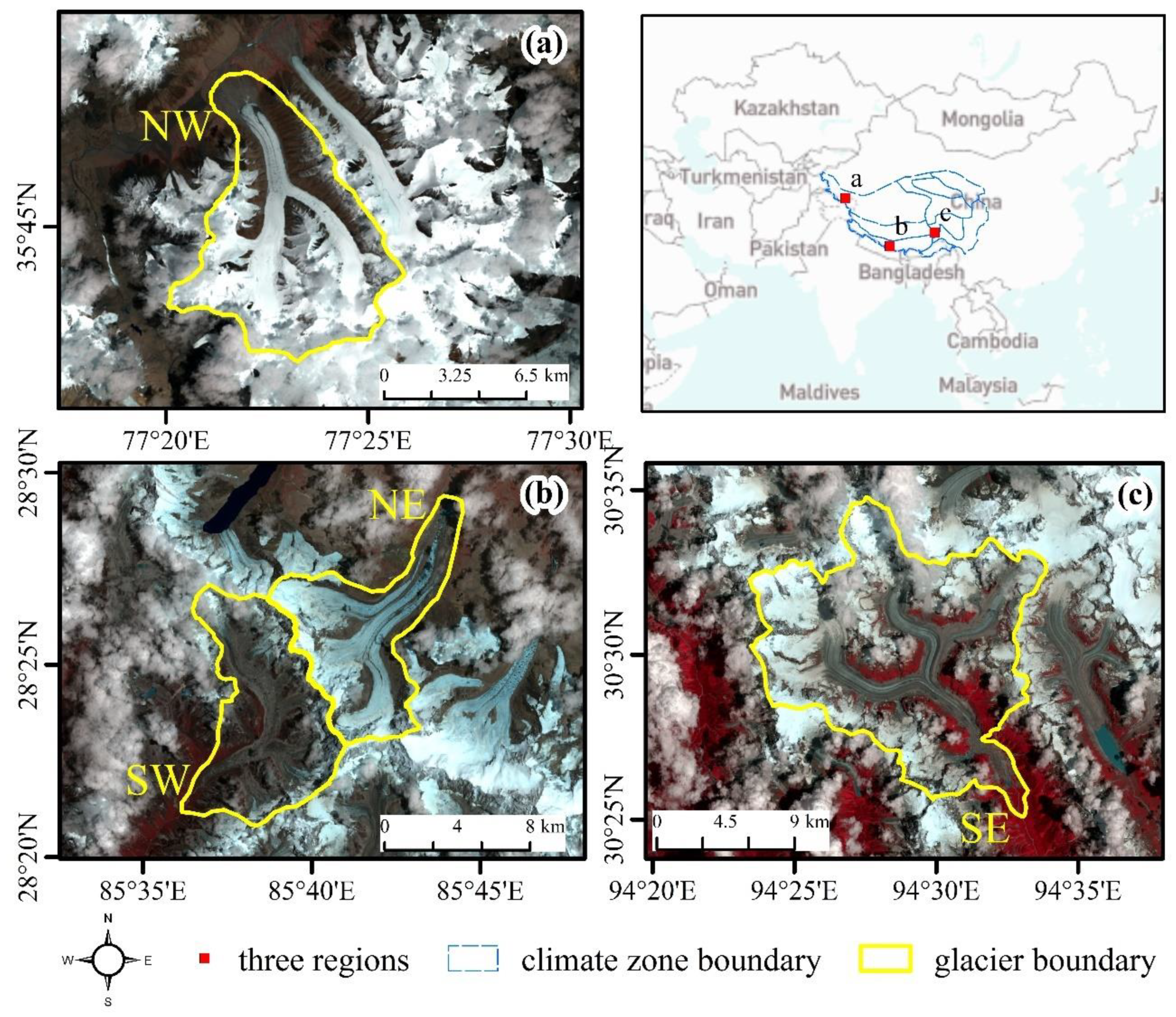
Figure 1. The topography base map of the Tibetan Plateau (TP) with three insets showing four glaciers in three different climatic zones. The four glaciers were selected as our study sites based on the main aspect of the glacier flow line. The black polygons show the boundaries of the different climatic zones on the Tibetan Plateau (14 June 2020). The red squares a-c in the upper-right diagram correspond to the glaciers in each of the three climate regions, as shown in figures (ac).
Remotesensing 14 01980 g001
Figure 2. Line charts of the elevation, slope, and aspect distribution of the four glaciers. The black, red, green, and blue curves are for the NW, NE, SW, and SE glaciers, respectively.
Remotesensing 14 01980 g002
Figure 3. The flowchart for data processing. The dashed red box indicates the pre-processing of the radar data, and the blue dashed box indicates the generation of multiple data suites of backscattering coefficients, polarization decomposition parameters, and interferometric coherence coefficient. Five land surface classes are obtained from the integrated machine learning classification algorithm.
Remotesensing 14 01980 g003
Figure 4. Illustration of the integrated machine learning classification method. Different colored circles represent samples of various land surface types.
Remotesensing 14 01980 g004
Figure 5. Spatial relationship between aspect-beam angle δ, pixel’s aspect, and radar beam direction, where θ in red is the angle between the satellite orbit and north, which is 8.18 degrees for Sentinel-1A. The straight black line and arrow represent the aspect and are described in black font. The blue line and arrow indicate the satellite azimuth and range direction, respectively. (a,b) correspond to the ascending and descending nodes, respectively.
Remotesensing 14 01980 g005
Figure 6. The statistics of the aspect-beam angle for the four glaciers. Each histogram corresponds to a glacier, with the x-axis corresponding to four subranges of the aspect-beam angle (S, M_r, M_l, L) and three secondary statistical parameters (PD_V, SD_H, SD_V), and the y-axis corresponding to the ratio of the respective pixel area to the total glacier area. The orange and blue bars indicate the ascending and descending nodes, respectively.
Remotesensing 14 01980 g006
Figure 7. The classification prediction accuracy for the four glaciers using the machine learning algorithms of the classifier classes in the MATLAB Classification Learner module. (a) The average prediction accuracy of the four classifier classes for four glaciers. (b) The prediction accuracy of the 20 MATLAB machine learning classification algorithms for the four glaciers. Each row represents one glacier, and each column corresponds to one classifier class. See Table 3 for the correspondence between algorithm number and name.
Remotesensing 14 01980 g007
Figure 8. Comparison of the average prediction accuracy and actual accuracy of the four optimal algorithms, the numbers on the x-axis correspond to the algorithms in Table 3. The three algorithm quality indices for evaluation are MAE, RMSE, and mean error.
Remotesensing 14 01980 g008
Figure 9. Classification results of the four glaciers from the four BC data suites (see Table 4). Each row corresponds to a BC suite of a specific orbit node and co/cross-polarization mode. Each column corresponds to a glacier or glaciers. The NE and SW glaciers are displayed in the middle column since they are close.
Remotesensing 14 01980 g009
Figure 10. Classification results of the four glaciers from the two PDP data suites of both ascending (A) and descending (D) nodes.
Remotesensing 14 01980 g010
Figure 11. Glacier classification results of four glaciers from the four ICC data suites.
Remotesensing 14 01980 g011
Figure 12. (a) The correlation coefficient between any two layers in the BC, PDP, and ICC data suites. (b) The importance ranking of the seven layers in each of the BC, PDP, and ICC suites. The x-axis is the layers of each data suite (see Table 2), and the y-axis is the chi-square statistic value of the Kruskal–Wallis test, which represents the importance of the layer in the recognition of the surface type of the glacial area.
Remotesensing 14 01980 g012
Figure 13. False-color images of four glaciers. R, G, B channels correspond to the first three important layers of each data suite: For the BC suite, RGB = elevation, sigma naught, and sigma naught-based texture_3; for the PDP suite, RGB = elevation, anisotropy, and entropy; for the ICC suite, RGB = elevation, coherence coefficient and texture_2 from the coherence coefficient. The left and right sides are four glaciers corresponding to the ascending and descending nodes, respectively. Each row represents the co-polarization and cross-polarization of three data suites from top to bottom.
Remotesensing 14 01980 g013
Figure 14. Pearson correlation coefficients between glacier surface features and classification accuracy for the three data sets and p-value. The x-axis represents the four aspect-beam angle ranges and the three secondary statistical features (see Section 3.7). The left y-axis represents the Pearson correlation coefficient between each glacier surface feature and glacier classification accuracy, and the right y-axis represents the p-value corresponding to the Pearson correlation coefficient. The three histograms from top to bottom correspond to BC, PDP, and ICC suites.
Remotesensing 14 01980 g014
Table 1. Sentinel-1A images used for this study (A = Ascending D = Descending).
No.GlacierProduct Unique ID PathFrameIncidence
Angle (degree (°))
Acquisition Time
(MM/DD/2018 hh:mm)
Pass
Direction
1NW7BC912911231.19–54.0425 July 12:48A
22EF412911231.19–54.046 August 12:48A
3E52213647130.74–53.9526 July 0:49D
4764713647130.74–53.957 August 0:49D
5NE & SW9671858830.71–54.0922 July 12:22A
6CA6A858830.71–54.093 August 12:22A
7479E12149631.49–53.9625 July 0:10D
84E0412149631.49–53.966 August 0:10D
9SEDBB870128231.24–54.1321 July 11:41A
1020B870128231.24–54.132 August 11:41A
119F697749031.33–54.0521 July 23:45D
12C16C7749031.33–54.042 August 23:45D
Table 2. Parameters (layers) included in each of the three data suites.
BC SuitePDP SuiteICC Suite
layer 1sigma naughtentropycoherence coefficient
layer 2sigma naught_based texture_1anisotropycoherence coefficient_based texture_1
layer 3sigma naught_based texture_2alphacoherence coefficient_based texture_2
layer 4sigma naught_based texture_3VV/VH ratiocoherence coefficient_based texture_3
layer 5local incident anglelocal incident anglelocal incident angle
layer 6elevationelevationelevation
layer 7slopeslopeslope
Table 3. Four classifier classes and 20 machine learning classification algorithms in the MATLAB classification learner module.
No.AlgorithmClassifier Class
1Fine TreeDecision Trees
2Medium Tree
3Coarse Tree
4Linear SVMSupport Vector Machines
5Quadratic SVM
6Cubic SVM
7Fine Gaussian SVM
8Medium Gaussian SVM
9Coarse Gaussian SVM
10Fine KNNNearest Neighbor Classifiers
11Medium KNN
12Coarse KNN
13Cosine KNN
14Cubic KNN
15Weighted KNN
16Boosted TreesEnsemble Classifiers
17Bagged Trees
18Subspace Discriminant
19Subspace KNN
20RUSBoosted Trees
Table 4. Comparison between the overall accuracy and the prediction accuracy of the optimal model for four glaciers under different data suites.
GlacierAlgorithmBCPDPICC
A_VVA_VHD_VVD_VHADA_VVA_VHD_VVD_VH
NWCoarse Gaussian SVM 74.70
Boosted Trees 99.80 99.80
Bagged Trees 98.90
Subspace KNN99.9099.9099.7099.70 99.30 99.70
Error *0.04 −0.07 −0.17 −0.68 0.270.10 −3.59 −0.30−0.23−0.06
NEBagged Trees98.40 98.60 98.50 97.00 96.10 96.5096.50 96.60 96.70
Subspace KNN 98.20
Error0.080.60.13−0.49−0.230.160.74−0.08−54.90 −56.64
SWFine Tree67.1067.0066.3066.20 65.4065.2068.5067.6068.4067.50
Error−1.88−11.15 −0.94−1.31−1.49−1.79 −1.08 −0.66−1.18−0.92
SEBagged Trees97.1098.0097.3098.10 96.9096.3096.7096.40
Subspace KNN 96.8096.20
Error0.220.070.430.35−0.080.740.700.650.580.27
* Error represents the actual classification accuracy of each algorithm minus the prediction accuracy, a positive value indicates that the actual classification accuracy is higher than the prediction accuracy, and vice versa.
Publisher’s Note: MDPI stays neutral with regard to jurisdictional claims in published maps and institutional affiliations.